Image informative maps for componentwise estimating parameters of signal-dependent noise - SPIE ...
←
→
Page content transcription
If your browser does not render page correctly, please read the page content below

Image informative maps for component-
                 wise estimating parameters of signal-
                 dependent noise

                 Mykhail L. Uss
                 Benoit Vozel
                 Vladimir V. Lukin
                 Kacem Chehdi

Downloaded From: https://www.spiedigitallibrary.org/journals/Journal-of-Electronic-Imaging on 10 Jun 2022
Terms of Use: https://www.spiedigitallibrary.org/terms-of-use
Journal of Electronic Imaging 22(1), 013019 (Jan–Mar 2013)

                    Image informative maps for component-wise estimating
                             parameters of signal-dependent noise
                                                                             Mykhail L. Uss
                                                                       National Aerospace University
                                                          Department of Aerospace Radioelectronic Systems Design
                                                                  17 Chkalova Street, Kharkov, Ukraine

                                                                                 Benoit Vozel
                                                                 IETR UMR CNRS 6164-University of Rennes 1
                                                                             Lannion cedex, France
                                                                      E-mail: benoit.vozel@univ-rennes1.fr

                                                                               Vladimir V. Lukin
                                                                          National Aerospace University
                                                                             Department of Receivers
                                                                        Transmitters and Signal Processing
                                                                       17 Chkalova Street, Kharkov, Ukraine

                                                                             Kacem Chehdi
                                                                 IETR UMR CNRS 6164-University of Rennes 1
                                                                          Lannion cedex, France

                                                                                                    (STD)] from image data has been extensively studied by
                Abstract. We deal with the problem of blind parameter estimation
                of signal-dependent noise from mono-component image data.                           researchers for the last decade (see Ref. 1 and references
                Multispectral or color images can be processed in a component-                      therein). For a given sensor, the problem is to estimate
                wise manner. The main results obtained rest on the assumption                       noise parameters directly from noisy images acquired by
                that the image texture and noise parameters estimation problems                     this sensor.2–15
                are interdependent. A two-dimensional fractal Brownian motion                           Sensor noise must be detected and quantified prior to the
                (fBm) model is used for locally describing image texture. A polynomial
                model is assumed for the purpose of describing the signal-dependent
                                                                                                    majority of subsequent image processing tasks. Such infor-
                noise variance dependence on image intensity. Using the maximum                     mation can help to properly select a suitable technique or
                likelihood approach, estimates of both fBm-model and noise param-                   adjust a method parameter to a current noise level (unknown
                eters are obtained. It is demonstrated that Fisher information (FI) on              in advance), with the final goal of making these techniques
                noise parameters contained in an image is distributed nonuniformly                  operate well enough. For example, different image filtering
                over intensity coordinates (an image intensity range). It is also
                shown how to find the most informative intensities and the corre-
                                                                                                    methods are needed to deal with either additive (signal-
                sponding image areas for a given noisy image. The proposed estima-                  independent) noise (see Ref. 16 and references therein) or
                tor benefits from these detected areas to improve the estimation                    signal-dependent Poisson noise [typical for charge-coupled
                accuracy of signal-dependent noise parameters. Finally, the potential               device (CCD) sensors].17–28 A threshold that is a function of
                estimation accuracy (Cramér-Rao Lower Bound, or CRLB) of noise                      noise standard deviation can be used with an edge detector.13
                parameters is derived, providing confidence intervals of these esti-                In Refs. 29 and 30, a method is proposed for estimating the
                mates for a given image. In the experiment, the proposed and existing
                state-of-the-art noise variance estimators are compared for a large                 denoising bounds for nonlocal filters from a noisy image,
                image database using CRLB-based statistical efficiency criteria.                    where noise statistics are to be known or accurately pre-
                © The Authors. Published by SPIE under a Creative Commons                           estimated from the same noisy data. Similar results for local
                Attribution 3.0 Unported License. Distribution or reproduction of                   filters were obtained in Ref. 31, with the same requirement
                this work in whole or in part requires full attribution of the original             for noise statistics.
                publication, including its DOI. [DOI: 10.1117/1.JEI.22.1.013019]                        A signal-independent spatially uncorrelated noise model
                                                                                                    was the first possibility widely considered in the literature
                                                                                                    for modeling sensor noise in a very large number of image
                1 Introduction                                                                      processing applications. In these applications, the noise is
                A challenging problem of blind estimation of inherent sensor                        typically assumed as a zero mean stationary Gaussian distrib-
                noise parameters [mainly its variance or standard deviation                         uted random process. Such process is fully described in
                                                                                                    terms of second-order statistics: its variance or standard
                                                                                                    deviation and a two-dimensional (2-D) Dirac delta function
                Paper 12159 received May 2, 2012; revised manuscript received Dec. 8,               for its spatial autocorrelation function. For such noise
                2012; accepted for publication Jan. 11, 2013; published online Feb. 1, 2013.        models, the methods designed for estimating noise standard

                Journal of Electronic Imaging                                              013019-1                                        Jan–Mar 2013/Vol. 22(1)

Downloaded From: https://www.spiedigitallibrary.org/journals/Journal-of-Electronic-Imaging on 10 Jun 2022
Terms of Use: https://www.spiedigitallibrary.org/terms-of-use
Uss et al.: Image informative maps for component-wise estimating parameters. . .

                deviation can be roughly divided into two groups: the meth-                         nonuniform and may include different texture patterns,
                ods operating in the spatial domain and those operating in the                      edges, objects of small size, etc. All these heterogeneities
                spectral domain. Spatial methods, also called homogeneous                           should not essentially influence the performance of a
                area (HA) methods,32 make an essential use of image homo-                           noise parameter estimator; i.e., estimated bias and standard
                geneous areas characterized by a negligible level of texture                        deviation should not increase significantly (over a theoreti-
                spatial variation compared to the noise level. Spectral meth-                       cal limit).
                ods utilize a suitable orthogonal transform to better separate                          Potentially, the performance of blind methods can be very
                image texture and noise; the former is assumed to be                                high—certainly higher than that of a human operator. The
                smoother compared to image noise.33 They can have certain                           reason is that these methods can use subtler differences
                advantages compared to spatial methods, as the latter also                          between image content and noise, which might be not visible
                can be applied to nonintensive texture, in addition to homo-                        to the human eye. But satisfying the above requirements al-
                geneous areas. In Refs. 15, 34–36, the estimation of additive                       together (and reaching a high level of estimation accuracy)
                noise standard deviation is performed by analyzing the                              for signal-dependent noise has been a difficult problem.12
                observed data in blocks of fixed size in the discrete cosine                            Extended versions of approaches, originally proposed
                transform (DCT) domain. Estimation using wavelet trans-                             for the estimation of signal-independent noise standard
                form is also possible.37,38                                                         deviation, have been considered to deal with signal-
                    However, with advances in CCD-sensor technology, the                            dependent noise, among them the well-known scatterplot
                applicability of the signal-independent noise model is dimin-                       approach.39 Recall that a scatterplot is a collection of points,
                ishing, and signal-dependent photonic noise is becoming                             each representing image local variance versus local mean. To
                more and more dominant.14,39 Nevertheless, the level of sig-                        reduce the influence of outliers, a robust fit to the scatterplot
                nal-independent thermal noise remains nonnegligible. Then,                          data points has typically been considered by different authors
                one has to deal with mixed signal-independent and signal-                           (e.g., Refs. 8, 10, and 39). Unfortunately, robust fit in the
                dependent noise, which, in general, can also be treated as                          presence of a large percentage of abnormal local variance
                signal-dependent. Such noise is intrinsically nonstationary,                        estimates (obtained from heterogeneous fragments) may
                but it can be locally approximated by stationary additive                           appear very unstable. As a result, different fit strategies can
                noise, with variance being a function of image intensity.                           lead to notably different estimation results.12
                In this case, the dependence of local variance on image inten-                          To meet all the requirements discussed above, we extend
                sity (called noise level function, or NLF, in Ref. 10) is of                        here the promising approach that we recently proposed in
                interest. If this dependence can be approximated by a poly-                         Ref. 15 to estimate the standard deviation (or variance) of
                nomial, then one has to estimate the parameters (coefficients)                      signal-independent noise (assumed to be spatially uncorre-
                of such a polynomial. For CCD-sensor noise, a first-order                           lated). Our approach introduces two specific maps: the
                polynomial is considered to be a proper model40 character-                          image texture informative (TI) map and the noise informative
                ized by two parameters, later referred to as signal-indepen-                        (NI) map. These two maps are complementary; i.e., for a
                dent and signal-dependent component variances.                                      given image, each scanning window (SW) belongs to one
                    It is important to mention that signal-dependent noise is                       or another map. Assigning a given SW to one of these
                significantly more restrictive compared to signal-independent                       maps is decided based on the Fisher information (FI) on
                noise: homogeneous areas of sufficient size, with intensities                       image texture parameters and noise standard deviation con-
                covering the whole image intensity range, are needed to accu-                       tained in this single window. In the NI map, a large amount
                rately estimate noise variance as a function of image intensity.                    of FI on the noise standard deviation is contained in each
                This problem was addressed, for example, in Ref. 10, where a                        selected SW forming this map. Such SWs contribute in solv-
                priori information on an estimated nonlinear NLF was used to                        ing the main task, i.e., the accurate blind estimation of noise
                compensate for the lack of homogeneous areas and to stabilize                       parameters. On the contrary, in the TI map, a large amount of
                the estimation process. Note that such a priori information is                      FI on image texture parameters is contained in corresponding
                not available for all sensors. In this situation, the estimation of                 SWs. Such SWs are involved in solving an auxiliary task
                noise parameters (coefficients of a polynomial and signal-                          (i.e., the estimation of image texture parameters).
                independent and signal-dependent component variances)                                   Note that both tasks are not mutually exclusive since
                should be performed in a blind manner, relying only on                              texture parameters for NI SWs and noise parameters for TI
                observed noisy data. To reach high performance in such a sit-                       SWs remain unknown, due to mutual masking of texture
                uation, a blind noise parameter estimator should satisfy the                        and noise. Therefore, the core of our approach is to use
                following requirements:1                                                            both maps simultaneously in an iterative manner. Noise param-
                                                                                                    eters are estimated from NI SWs and then are applied to
                    1. To provide unbiased estimates with as little variance as                     improve the estimation accuracy of texture parameters from
                       possible.                                                                    neighboring TI SWs. The latter parameters, in turn, are used
                    2. To perform well enough at different noise levels.                            to improve the estimation accuracy of noise parameters.
                    3. To be insensitive to image content; i.e., to provide                             To implement this scheme, we carry out the maximum
                       appropriate accuracy, even for textural images.                              likelihood (ML) estimation of a parametrical 2-D fractal
                                                                                                    Brownian motion (fBm) model, selected for describing
                   By saying “with as little variance as possible,” we mean                         locally the texture of a 2-D noisy image SW. The FI on the
                that there is a certain theoretical limit on the estimation accu-                   estimated parameter vector (including fBm-model parame-
                racy (in terms of standard deviation) of noise parameters                           ters and noise standard deviation) can then be derived. To
                from image data.15 It is desirable for an estimator to perform                      obtain the final estimation of noise standard deviation from
                close to this limit. The true image content is certainly                            the NI map, two alternatives, either fBm- or DCT-based

                Journal of Electronic Imaging                                              013019-2                                          Jan–Mar 2013/Vol. 22(1)

Downloaded From: https://www.spiedigitallibrary.org/journals/Journal-of-Electronic-Imaging on 10 Jun 2022
Terms of Use: https://www.spiedigitallibrary.org/terms-of-use
Uss et al.: Image informative maps for component-wise estimating parameters. . .

                estimators (NI þ fBm, NI þ DCT), are proposed. The first                               By yðt; sÞ, t ¼ 1: : : N c , and s ¼ 1: : : N r , we denote a sin-
                one performs direct parametrical ML estimation of noise                             gle-component image with N c columns and N r rows (for
                standard deviation from NI SWs, with a texture correlation                          multi-component or color images, the approach proposed
                matrix defined according to the fBm model and parameters                            here should be applied component-wise). Suppose that the
                derived from neighboring TI SWs. The second one applies                             image yðt; sÞ is affected by signal-dependent noise according
                DCT transform to NI SWs and uses only a fixed and limited                           to the following model:
                number of high-frequency DCT coefficients to estimate
                noise standard deviation.                                                                             yðt; sÞ ¼ xðt; sÞ þ n½t; s; xðt; sÞ;                     (2)
                   Now, under signal-dependent noise hypothesis, the main
                difficulty is to take into account the variation of noise standard                  where xðt; sÞ is the original noise-free image, n½t; s; xðt; sÞ is
                deviation with regard to image intensity (due to the signal-de-                     an ergodic Gaussian noise with zero mean, signal-dependent
                pendent noise component), while still resorting to image NI/TI                      variance σ 2n ½xðt; sÞ and a 2-D Dirac delta function for its spa-
                maps. For this purpose, we analyze how image NI SWs are                             tial autocorrelation function. For a general case, for signal-
                distributed over the intensity range. This distribution allows                      dependent noise variance σ 2n ðIÞ, we assume a polynomial
                the finding of narrow intensity intervals where noise variance                      model with degree np : σ 2n ðI; cÞ ¼ c ⋅ ½1; I; I 2 ; : : : ; I np , where
                can be accurately estimated and the discarding of noninforma-                       I is true image intensity and c ¼ ðc0 ; c1 ; : : : ; cnp Þ is a coef-
                tive intensities (those without any NI SW detected). Final                          ficient vector of size ðnp þ 1Þ × 1.
                estimates of noise signal-independent/dependent component                               However, in the section of this paper that describes the
                variances are obtained by linear fit applied to these accurate                      experiment, we concentrate on a reduced-order noise
                variance estimates localized with regard to intensity. The                          model for recent CCD sensors. In this case, the noise
                whole procedure ensures the absence of outliers among                               n½t; s; xðt; sÞ is supposed to be the sum of two components:
                local estimates of noise variance. Therefore, robust fit proce-                     n½t; s; xðt; sÞ ¼ nSI ðt; sÞ þ nSD ½t; s; xðt; sÞ. The first one,
                dures that can be unstable are no longer needed.                                    nSI ðt; sÞ, is signal-independent with variance σ 2n:SI , and the
                   This paper is organized as follows. Section 2 briefly intro-                     second one, nSD ½t; s; xðt; sÞ, is signal-dependent with vari-
                duces the fBm model and then recalls NI þ fBm and NI þ                              ance σ 2n:SD ⋅ I (Poisson-like noise). This corresponds to a pol-
                DCT signal-independent noise variance estimators that we                            ynomial model of the first order (np ¼ 1) and, thus the
                previously proposed. Later in this section, the signal-depen-                       coefficient vector simply reduces to c ¼ ðσ 2n:SI ; σ 2n:SD Þ:
                dent noise parameter estimation problem is introduced from
                an informational point of view, including FI distribution over                              σ 2n ðIÞ ¼ ðσ 2n:SI ; σ 2n:SD Þ ⋅ ½1; I ¼ σ 2n:SI þ σ 2n:SD ⋅ I:   (3)
                the available intensity range for a given image. In Sec. 3,
                NI þ fBm and NI þ DCT estimators are extended for sig-
                nal-dependent noise and the potential accuracy of such
                noise parameter estimates is provided. In Sec. 4, the perfor-                       2.2 Structure of NI þ fBm and NI þ DCT Signal-
                mance of NI þ fBm and NI þ DCT estimators is compara-                                    Independent Noise Variance Estimators
                tively assessed against two other modern methods in a large                         At this point, let’s briefly recall the main ideas suggested in
                image database and real noise from a CCD sensor. Finally, in                        the NI þ fBm and NI þ DCT signal-independent noise vari-
                the last section, conclusions are offered.                                          ance estimators (σ 2n:SD ¼ 0) proposed by the authors in
                                                                                                    Ref. 15. Their generalized structure is recalled in Fig. 1.
                                                                                                    This structure used the fBm model and both image NI
                2 Signal-Dependent Noise Parameters Estimation                                      and TI maps. In the estimation process, a processed sample
                  from Noise and TI Maps                                                            corresponds to a noisy textural fragment or SW of the image.
                                                                                                    The sample is described by a statistical parametrical model.
                2.1 FBm Model for Describing Texture Locally
                                                                                                    The model parameters vector includes both texture parame-
                To describe image texture locally, we propose to use the fBm                        ters (fBm-model parameters) and signal-independent noise
                model BH ðt; sÞ. Fractal analysis based on mathematical fBm                         variance σ 2n:SI . After initialization (stage 1), NI/TI maps
                processes has been suggested as a useful technique for char-                        and noise standard deviation are simply assumed to be
                acterizing real-life images, as they can describe quite com-                        equal to initial guesses or current refined estimates in
                plicated textures or shapes of natural scenes with a minimal                        stage 2. At this stage, texture parameters are estimated for
                parameter set.41                                                                    each TI SW first. Then, these estimates act as texture param-
                   By definition, BH ðt; sÞ, H ∈ ½0;1, is a Gaussian process                       eter estimates in neighboring NI SWs. This stage results in
                [the original coordinates are at the point (0,0): BH ð0; 0Þ ¼ 0]                    estimates of the parameter vectors for all SWs for further use
                with the correlation function:42                                                    in stage 3.
                                                                                                       In stage 3, those SWs that can be efficiently used for esti-
                hBH ðt; sÞ · BH ðt1 ; s1 Þi                                                         mating either noise or texture parameters are identified. We
                              pffiffiffiffiffiffiffiffiffiffiffiffiffiffi             qffiffiffiffiffiffiffiffiffiffiffiffiffiffi2H
                                                 2H                                                 propose to perform this task by considering the correspond-
                    ¼ 0.5σ 2x      t2 þ s2 þ t21 þ s21                                              ing FI on involved parameters or, equivalently the Cramér-
                          qffiffiffiffiffiffiffiffiffiffiffiffiffiffiffiffiffiffiffiffiffiffiffiffiffiffiffiffiffiffiffiffiffiffiffiffiffiffiffi2H                               Rao Lower Bound (CRLB), to each SW. By setting a proper
                        − ðt − t1 Þ2 þ ðs − s1 Þ2                      :                 (1)        threshold on CRLB, it becomes possible to find a subset of
                                                                                                    NI/TI SWs that provide noise/texture parameters estimates
                                                                                                    with a predefined accuracy. Finally, in stage 4, the noise stan-
                   In spatial terms, the Hurst exponent H describes fBm-                            dard deviation is estimated for each NI SW using either a
                texture roughness (H → 0 for rough texture, H → 1 for                               fBm-model-based ML estimator (NI þ fBm) or DCT
                smooth),43 and σ x describes fBm amplitude.                                         (NI þ DCT). Note that by using only NI SWs ensures

                Journal of Electronic Imaging                                              013019-3                                                     Jan–Mar 2013/Vol. 22(1)

Downloaded From: https://www.spiedigitallibrary.org/journals/Journal-of-Electronic-Imaging on 10 Jun 2022
Terms of Use: https://www.spiedigitallibrary.org/terms-of-use
Uss et al.: Image informative maps for component-wise estimating parameters. . .

                                                       Fig. 1 Structure of NI þ fBm and NI þ DCT SI noise variance estimators.

                that all individual noise standard deviation estimates in stage                     where
                4 achieve a predefined accuracy and that there are no outliers
                                                                                                                                            I σx σx   Iσx H
                among them. As a result, a simple nonrobust estimation pro-                                                   IfBm ¼
                                                                                                                                            I σx H    I HH
                cedure (for example, weighted mean) is sufficient in stage 4
                to obtain the final estimate σ^ 2n:SI .
                                                                                                    is information on fBm-model parameters, I σn σn is informa-
                                                                                                    tion on signal-independent noise standard deviation, and
                                                                                                    IfBm:σn ¼ ðI σx σn I Hσ n Þ is mutual information.
                2.3 FI Distribution over Images
                                                                                                        Assume that noise-informative SWs have been detected,
                When solving the estimation problem for signal-independent                          and assign mean intensity Ī i to the ith NI SW. For the subset
                noise, the total amount of FI on noise standard deviation con-                      N SW ≥ 1 of these windows with Ī i ∈ ½I − ΔI∕2; I þ ΔI∕2,
                tained in all noise-informative SWs determines the potential                        we assume a signal-independent noise model with standard
                performance of an estimator (in terms of its variance).15 For                       deviation σ n ¼ σ n ðIÞ. Then, joint FI matrix Iθ ðI; ΔIÞ on
                signal-dependent noise, when noise standard deviation is a                          extended parameter vector θ ¼ ðσ x.1 ; H 1 ; σ x.2 ; H 2 ; : : : ;
                function of true image intensity, the distribution of FI                            σ x:N SW ; HN SW ; σ n Þ can be obtained in a similar way:
                over the image intensity range becomes of major importance.
                                                                                                                       0                                                    1
                Specifically, if all noise-informative SWs have the same                                                     IfBm.1 : : :           0         IfBm:σ n .1
                intensity mean I 0 , only the value of σ n ðI 0 Þ can be estim-                                        B :::            :::        :::           :::        C
                                                                                                      Iθ ðI; ΔIÞ ¼ B   @ 0
                                                                                                                                                                            C;
                ated. This allows estimating the pure Poisson-like                                                                      :::     IfBm:N SW    IfBm:σ n :N SW A
                (σ 2n ðIÞ ¼ σ 2n:SD I) or multiplicative (σ 2n ðIÞ ¼ σ 2μ I 2 ) signal-de-
                                                                                      pffiffiffiffi                                ITfBm:σ n .1 : : : ITfBm:σn :N SW I σn σn :N SW
                pendent noise standard deviation by σ^ n:SD ¼ σ^ n ðI 0 Þ∕ I 0
                and σ^ μ ¼ σ^ n ðI 0 Þ∕I 0 , respectively (with accuracy that does                                                                                             (4)
                not depend on I 0 ). If a mixture of signal-independent                                                        PN SW
                noise and either Poisson-like or multiplicative noise is                            where I σn σn :N SW ¼ j¼1 I σn σn :j . From the matrix Iθ ðI; ΔIÞ,
                assumed, the best accuracy can be achieved when FI is dis-                          CRLB on σ n can be found to be the corresponding element
                tributed equally between two intensities, I min and I max , with                    of the inverse matrix Iθ ðI; ΔIÞ−1 (marked by “n” in the lower
                I max − I min being as large as possible. When no a priori                          index below):
                information about σ n ðIÞ is available, then FI uniformly dis-
                tributed over all image intensity ranges is the best option.                                                 σ 2σn ðI; ΔIÞ ¼ Iθ ðI; ΔIÞ−1
                                                                                                                                                       n :                     (5)
                     Unfortunately, for a particular image, this distribution
                cannot be modified. What can be done, in practice, is to                               Using σ 2σn ðI; ΔIÞ, we define CRLB per unit intensity
                establish the actual distribution for a given image and to                          range ½I − 0.5; I þ 0.5 as
                obtain the corresponding accuracy of noise parameter vector
                c estimation, taking into account available a priori informa-                                               Δσ 2σn ðIÞ ¼ ΔI ⋅ σ 2σ n ðI; ΔIÞ;                  (6)
                tion. This problem will be addressed next, and NI þ fBm and
                NI þ DCT estimators will be extended to estimate the                                and relative CRLB per unit intensity range as
                σ n ðI; cÞ function.                                                                        Δσ 2σ n :rel ðIÞ ¼ Δσ 2σn ðIÞ∕σ n ðIÞ ¼ ΔI ⋅ σ 2σn :rel ðI; ΔIÞ;   (7)
                     The corresponding FI about the parameter vector
                θ ¼ ðσ x ; H; σ n Þ on texture parameters ðσ x ; HÞ and noise                       where σ σn :rel ðI; ΔIÞ ¼ σ σn ðI; ΔIÞ∕σ n ðIÞ.
                standard deviation ðσ n Þ was introduced in Ref. 15 for a single                       To get better insight on the meaning of variables defined
                SW (N SW ¼ 1) as                                                                    above, the possible shape of Δσ 2σn :rel ðIÞ and its relation to the
                                                                                                  image content are illustrated in Fig. 2. Figure 2(a) displays
                                                 IfBm ITfBm:σn
                                       Iθ ¼                         ;                               the green component of image 3 from the NED2012 color
                                                IfBm:σn I σn σn                                     images database (Noise Estimation Database), later referred

                Journal of Electronic Imaging                                              013019-4                                                       Jan–Mar 2013/Vol. 22(1)

Downloaded From: https://www.spiedigitallibrary.org/journals/Journal-of-Electronic-Imaging on 10 Jun 2022
Terms of Use: https://www.spiedigitallibrary.org/terms-of-use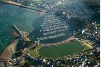
Uss et al.: Image informative maps for component-wise estimating parameters. . .

                Fig. 2 (a) Green component of image #3 from the NED2012 database; (b) relative CRLB per unit intensity range, Δσ 2σ n :rel ðIÞ, versus intensity for
                image #3 from the NED2012 database (test image) degraded with signal-dependent noise.

                to as the test image. We created the NED2012 database espe-                         sufficiently accurate noise standard deviation estimates.
                cially for testing the noise parameter estimator. It is described                   Conversely, for informative image intensities with low
                in detail in Sec. 4.1, later in this article.                                       Δσ 2σ n :rel ðIÞ (areas 1–4 in Fig. 2), the same accuracy can be
                   The Δσ 2σ n :rel ðIÞ function has been calculated for the test                   achieved for smaller ΔI k. It is natural to estimate noise
                image, and it is displayed in Fig. 2(b). In this experiment,                        standard deviation with a predefined accuracy σ 2σn ðI; ΔIÞ ¼
                we fix ΔI ¼ 1 to calculate Δσ 2σn :rel ðIÞ. A way to calculate                      σ 2n:rel: max for each considered intensity interval Ik ; i.e., to
                ΔI automatically will be described in Sec. 3.1. Intensities                         require
                of the test image cover range approximately from 0 to
                1,200. In Fig. 2(b), four image intensity intervals with the                                                  σ 2σn :rel ðĪ k ; ΔI k Þ ≤ σ 2n:rel: max ;                 (9)
                lowest Δσ 2σ n :rel ðIÞ can be seen, with image intensities around
                10 (1), 200 (2), 400 (3), and 800 (4).                                              where Ī k ¼ ðI max :k þ I min :k Þ∕2 is the center of interval Ik .
                   Objects in the test image with intensities falling within                        Eq. (9) is an extension of the thresholding procedure used
                intervals 1–4 are marked in Fig. 2(a) with the corresponding                        in Ref. 15 to select a given SW as NI in the signal-independent
                numbers. Interval 1 corresponds to the nonintensive dark tree                       noise case. Whereas this original constraint requires the sig-
                texture, intervals 2 and 3 relate to homogeneous house fronts,                      nal-independent noise standard deviation to be estimated with
                and interval 4 relate to cloudy sky. One can see that
                                                                                                    a predefined accuracy from a single NI SW, Eq. (9) requires
                Δσ 2σn :rel ðIÞ indicates image areas that provide accurate
                                                                                                    the same standard deviation estimation, but from the subset of
                noise standard deviation estimation and their localization
                                                                                                    NI SWs with mean intensities within the interval Ik .
                with regard to image intensity.
                                                                                                       According to Eq. (6), for an arbitrary intensity Ī k ¼ I,
                                                                                                    equality in Eq. (9) holds for
                3 NI  FBm and NI  DCT Estimators for
                  Signal-Dependent Noise Parameters                                                                     ΔI k ¼ ΔI ¼ Δσ 2σn :rel ðIÞ∕σ 2n:rel: max :                      (10)
                3.1 Preliminaries of the Proposed Estimators of                                         Therefore, ΔIðIÞ is just a scaled-down version of
                       Polynomial SD Noise Variance
                                                                                                    Δσ 2σ n :rel ðIÞ. In the example considered in Fig. 2, we set
                While designing the signal-dependent noise parameter esti-                          σ n:rel: max ¼ 0.1. For this value, ΔIðIÞ varies from 1 to 10
                mator, we assume piecewise-constant approximation to the                            in informative intensity intervals 1–4 and exceeds 200 in
                σ 2n ðIÞ function:                                                                  noninformative intervals [shown by the peaks in
                                                                                                    Fig. 2(a)]. It follows that for informative intensities, noise
                  σ 2n ðIÞ ¼ σ 2n:k ;   I ∈ Ik ¼ ½I min :k ; I max :k ;   k ¼ 1: : : K; (8)        variance can be accurately estimated from very narrow inten-
                                                                                                    sity intervals, enabling fine NLF analysis.
                where          Ik1 ∩ Ik2 ¼ ∅,         k1 ≠ k2 ,  I min :k ≥ I min and                   Based on Eq. (10), the set of intervals Ik is obtained by the
                I max :k ≤ I max , ½I min ; I max  is the available image intensity                following procedure:
                range.
                    As utilizing NI SWs along with either fBm-based or                                 1. Find    Ī     that         minimizes                       Δσ 2σn :rel ðIÞ:   Ī ¼
                DCT-based noise standard deviation estimators (NI þ fBm                                    argmin ½Δσ 2σ n :rel ðIÞ;
                or NI þ DCT) was proved to be efficient in Ref. 15 for                                      I min
Uss et al.: Image informative maps for component-wise estimating parameters. . .

                    5. Add a new interval to the list of intervals found at pre-                    specified in Ref. 15. It is equal to the minimum of sample
                       vious iterations. Increase K by unit.                                        standard deviation estimates over all image nonoverlapping
                    6. Repeat this process until no new pair ðĪ; ΔIÞ can be                        SWs. For the test image, the value σ^ 2n:SI:IG ≈ 170.60 was
                       found, and then terminate.                                                   obtained. The initial guess for the vector c assumes the initial
                                                                                                    value c^ IG ¼ ðσ^ 2n:SI:IG ; 0Þ.
                    For each interval Ik , σ^ 2n:k is estimated using either the                          Texture and noise parameter estimates and NI and TI
                NI þ fBm or the NI þ DCT estimator (under signal-indepen-                           maps are updated in stage 2. In this stage, we fix noise
                dent hypothesis). At the same time, σ σn :rel ðĪ k ; ΔI k Þ is calcu-              parameters to be equal to either an initial guess c^ i¼1 ¼ c^ IG
                lated for future use. The output of the proposed signal-                            or the previously estimated value c^ i ¼ c^ i−1 (here, i defines
                dependent noise estimator is the set of noise standard                              the iteration index). The signal-dependent noise variance
                deviation estimates σ^ 2n:k obtained for each interval Ik and                       for each SW (both NI and TI) is calculated according to
                the corresponding set of mean intensities Ī k .                                    the retained polynomial noise model (a mixture of signal-in-
                    Now, the maximum likelihood estimation (MLE) of coef-                           dependent and Poisson-like signal-dependent noises in this
                ficients vector c is obtained by                                                    case) as σ 2n ðI; c^ i Þ, substituting true image intensity by mean
                                                                                                    intensity over current SW. Then, fBm-model parameters for
                                                c^ ¼ A−1 b;                            (11)         TI and NI SWs are estimated, and discrimination between
                                                                                                    texture/NI SWs can be refined as specified in Ref. 15.
                where A is the Vandermonde matrix with elements Aij ¼                                     Next, in stage 3, a current value of relative CRLB per unit
                P iþj 2                P 2 i 2
                  k Ī k ∕σ σ 2 , bi ¼  k σ n:k Ī k ∕σ σ 2 , and σ σ 2n·k ¼ 2σ n ðĪ k Þ ·
                                                                                2                   image intensity (ΔI ¼ 1) Δσ 2σ n :rel ðIÞ and the corresponding
                              n:k                          n:k
                σ σn ·rel ðĪ k ; ΔI k Þ is the potential accuracy of the estimation                set of intervals Ik are calculated as described above. For illus-
                                                                                                    tration purposes, the Δσ 2σn :rel ðIÞ obtained in the first iteration
                of σ 2n:k . The correlation matrix of the estimate c^ has the fol-
                                                                                                    is shown in Fig. 4(a) as a straight black line.
                lowing form:                                                                              The set of intervals Ik allows the estimating of σ 2n:k values
                                                                                                    using either the fBm- or DCT-based estimator and refining
                                    σ2c ¼ hð^c − c0 Þð^c − c0 ÞT i ¼ A−1 ;             (12)
                                                                                                    the c^ estimate according to Eq. (11). The σ^ 2n:k estimates and
                where c0 is the true value of c vector.                                             σ 2n ðI; c^ i Þ function are both shown in Fig. 4(a) for the first
                                                                                                    iteration of the algorithm as black dots and a solid black
                                                                                                    line, respectively.
                3.2 Proposed Estimators of Polynomial SD Noise                                            The estimate σ 2n ðI; c^ i Þ is iteratively refined by repeating
                        Variance                                                                    stages 2–4 until convergence. The convergence of the algo-
                Note that the signal-dependent noise variance estimate                              rithm can be observed from the comparison of Fig. 4(a) with
                σ 2n ðI; c^ Þ obtained by Eq. (11) requires availability of the                     4(b), where the first and the final (fifth) iteration estimates of
                values of Δσ 2σn :rel ðIÞ and σ σ2n:k , that are based on true noise                Δσ 2σ n :rel ðIÞ, σ^ 2n:k , and σ 2n ðI; c^ i Þ for the test image are shown.
                variance σ 2n ðI; c0 Þ. Therefore, the signal-dependent noise                       Note that for each iteration, Fig. 4 shows σ 2n ðI; c^ i Þ estimates
                variance estimation procedure should operate iteratively as                         at the beginning of the iteration (signal-independent noise for
                described below. The structure of the proposed estimator                            the first iteration), not at the end. It can be seen that σ 2n:k esti-
                for texture parameters and signal-dependent noise standard                          mates are concentrated at intensities where Δσ 2σn :rel ðIÞ takes
                deviation is summarized in Fig. 3. In the following, we pro-                        on minimal values. Noise variance estimate σ 2n ðI; c^ i Þ for I
                vide a description of this estimator and illustrate its behavior                    from 600 to 1200 does not change significantly with itera-
                based on the test image [Fig. 2(a)] for np ¼ 1. True param-                         tions. Conversely, for I from 0 to 300 that corresponds to
                eter vector c0 ¼ ð5.0834; 0.1352Þ is obtained for this image                        areas (1) and (2) in Fig. 2(b), the noise variance estimate
                in the experiment via a calibration procedure (see Sec. 4.1 of                      decreases from about 170 [the first iteration, Fig. 4(a)] to
                this article for details).                                                          about 5 [the last iteration, Fig. 4(b)], and the number of
                      In the first stage, noise is assumed to be signal-                            σ^ 2n:k estimates decreases significantly (a smaller number of
                independent and an initial guess σ^ n:SI:IG is calculated as                        SWs is considered NI by the algorithm).

                    Fig. 3 Generalized scheme of proposed NI þ fBm and NI þ DCT estimators for image texture and signal-dependent noise parameters.

                Journal of Electronic Imaging                                              013019-6                                                  Jan–Mar 2013/Vol. 22(1)

Downloaded From: https://www.spiedigitallibrary.org/journals/Journal-of-Electronic-Imaging on 10 Jun 2022
Terms of Use: https://www.spiedigitallibrary.org/terms-of-use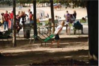
Uss et al.: Image informative maps for component-wise estimating parameters. . .

                             Fig. 4 Illustration of the signal-dependent noise estimation process by using the algorithm in Fig. 3 for the test image.

                   Now let us comment on the algorithm behavior for the                             provide a high estimation accuracy of signal-dependent noise
                textured area of the test image with an intensity close to                          variance. For images with not enough NI (homogeneous)
                60 (dark trees in the lower-right part of the test image).                          areas for estimating noise parameters, σ 2n ðI; c^ Þ may become
                With iterations, noise variance estimates are decreasing for                        inaccurate. Based on our experiments, we have found that
                this area. Consequently, the signal-to-noise ratio (measured                        this extreme case can always be detected by checking the
                locally) is constantly increasing. As a result, this area pro-                      accuracy of c^ at the current iteration or the entries of the
                gressively becomes less and less noise informative [this is                         σ2c matrix [see Eq. (12) for details].
                reflected by the increase of Δσ 2σn :rel ðIÞ function clearly
                seen in Fig. 4]. Finally, in iteration 5 [Fig. 4(b)], this area                     4 Experimental Results Using the NED2012
                is excluded from the noise variance estimation process (it                             Database
                becomes related to the TI map).                                                     This section deals with the application of the two designed
                   The results obtained at final iteration confirm that, given a                    estimators, NI þ fBm and NI þ DCT, of signal-dependent
                degraded image, Δσ 2σn :rel ðIÞ indicates that image areas that                     noise parameters to the NED2012 database of images that
                can provide accurate noise variance estimation and their                            have been corrupted by signal-dependent noise. Estimator
                localization with regard to image intensity. It can be clearly                      performance is analyzed and compared to that of the recently
                seen that the estimated curve σ 2n ðI; c^ Þ is very close to noise                  developed Automatic Scatterplot Reference Points Fitting
                variance σ 2n ðI; c0 Þ obtained by the calibration procedure. For                   with Restrictions (ASRPFR) method (discussed in Ref. 12)
                the considered test image, there are enough NI intensities to                       and the ClipPoisGaus_stdEst2D method published in Ref. 9.

                Journal of Electronic Imaging                                              013019-7                                         Jan–Mar 2013/Vol. 22(1)

Downloaded From: https://www.spiedigitallibrary.org/journals/Journal-of-Electronic-Imaging on 10 Jun 2022
Terms of Use: https://www.spiedigitallibrary.org/terms-of-use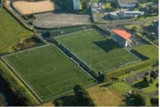
Uss et al.: Image informative maps for component-wise estimating parameters. . .

                   The primary goal of this study is to determine the                                  1. A series of 17 images of a white sheet of paper was
                potential accuracy of signal-dependent noise parameter                                    taken in raw Nikon electronic file format. For these
                estimation (variance of signal-independent and -dependent                                 images, we had a fixed International Standardization
                components) from real images of different types, and to                                   Organization (ISO) value (equal to 100), as well as
                compare the performance of existing estimators to this                                    other camera settings (using a manual regime), except
                bound.                                                                                    for shutter speed. By selecting different shutter speeds,
                                                                                                          a full image intensity range (in 12 bits) was covered.
                                                                                                          To suppress image texture (due to paper surface),
                4.1 Image Database for Testing Signal-Dependent                                           strongly defocused images were collected. Then paper
                     Noise Estimation Algorithms: NED2012                                                 texture was smoothed, leaving sensor noise unaffected.
                A key item in testing noise variance estimators is the avail-                          2. This series of images was partitioned into non
                ability of images with known noise parameters. Artificial                                 overlapping 8 × 8 SWs. A 2-D DCT transform was
                noise-free images with synthetic noise raise questions about                              then applied to each window. The highest 16 coeffi-
                the applicability of the obtained results to the real images                              cients (with indices from 5 to 8 for both dimensions)
                corrupted by real noise. Another possibility lies in using                                from each window were stored for further processing.
                real-life images with a low level of noise, with synthetic                                By relying on these high-frequency coefficients, we
                noise added for test purposes. In this area, the TID200844                                additionally diminished the influence of image texture.
                database has been extensively used.45 However, we have                                    For each such group of 16 coefficients, we calculated
                                                                                                          the image mean intensity in the corresponding SW.
                identified four drawbacks of TID2008 that prevent us from
                exploiting it in our study:                                                            3. The available intensity range from 0 to 4098 (12 bits)
                                                                                                          was divided into narrow intervals. DCT coefficients
                    1. Restricted image size. Indeed, the size of the images in                           were grouped according to their corresponding mean
                       the TID2008 database is 512 × 384 pixels. This corre-                              intensities. In this manner, for each kth intensity inter-
                       sponds to ≈0.2 Mpx. However, modern digital cam-                                   val, N DCT:k DCT coefficients were collected. The sam-
                       eras typically have more than 10 Mpx sensors.                                      ple variance of these N DCT:k coefficients, σ^ 2n:k , was an
                    2. Images from the TID2008 database are in 8-bit repre-                               estimate of the signal-dependent noise variance in k‘th
                       sentation, while 12 or 14 bits is typical currently for                            intensity interval.
                       images stored in raw format (for both digital cameras                           4. The coefficient vector           c was obtained by Eq. (11),
                                                                                                                                     pffiffiffiffiffiffiffiffiffiffiffiffiffiffiffiffi
                       and remote sensing acquisition systems).                                           with σ^ σ 2n:k ¼ 2σ^ 2n:k ∕ 2N DCT:k .
                    3. TID2008 images are subject to the demosaicing pro-
                                                                                                       Visual analysis of noise variance dependence on image
                       cedure to convert them from a color filter array (CFA)
                                                                                                    intensity shows notable deviation from the theoretic linear
                       to RGB representation. Demosaicing unfortunately
                                                                                                    shape (first-order polynomial), especially for the blue com-
                       affects the spectral properties of both image texture
                                                                                                    ponent (Fig. 5). To take this into account, the order of the
                       (due to smoothing) and inherent noise (because it
                       becomes spatially correlated). It is highly preferable                       approximation polynomial was set to np ¼ 2. The obtained
                       to deal with CFA representation to assess data directly                      estimates are given in Table 1 (we call them calibration
                       from a camera sensor.                                                        lines). The noise parameters obtained via the calibration pro-
                                                                                                    cedure will be marked with index “0” below.
                    4. TID2008 images contain inherent noise that, strictly                            It can be seen that the green channel is the least noisy
                       speaking, does not allow to consider them as noise-                          one, followed by the red and blue channels. Quadratic terms
                       free.15 This noise variance cannot be accurately esti-                       for all channels are nonzero. These values are statistically
                       mated due to issues 1 and 3. Automatic analysis                              significant (more than 0.704 · 10−5 ∕0.04924 · 10−5 or
                       shows that its variance is about 4,15 but manual analy-                      14.3 sigma) and cannot be neglected. They probably appear
                       sis shows it can locally reach 4 to 10. Such values are                      due to the internal regulations of the camera.
                       critical for our situation, as the standard deviation of                        For testing the two proposed estimators, we selected 25
                       the estimation error of additive noise variance pro-                         D80 images taken from the same camera during a two-year
                       vided by the NI þ DCT estimator (as we will show                             interval and organized them into the NED2012 database. The
                       next) can be as low as 0.2.                                                  database includes images with different content. Some of
                                                                                                    them have large homogeneous areas (e.g., sky), while others
                    To overcome these drawbacks, we have decided to base                            are quite textural, and defocused areas are present (Fig. 6).
                our study on 12-bit raw images from the Nikon D80 DSLR                              All images are presented as a CFA array of 2611×
                camera with a 10.2-Mpx CCD sensor. No extra noise was                               3900 pixels in size. Red, green, and blue channel data
                generated; we only dealt with the parameter estimation for                          were extracted from the CFA array by subsampling.
                noise that was originally present in D80 images. Our                                Images have different ISO values (from 100 to 320), different
                main assumption is that the noise parameters remain the                             shutter speeds (from 1∕1250 s to 1∕30 s), different apertures
                same with time and camera operational conditions.                                   (from f/4 to f/14) and different focal lengths (from 18 mm to
                Absence of noise spatial correlation is also assumed. Our                           135 mm). From this set of parameters, it is the ISO parameter
                experiments have shown no violation of these assumptions                            that directly affects noise parameters for both signal-inde-
                at the attained level of accuracy.                                                  pendent and -dependent components. In order to compensate
                    To accurately estimate true noise parameters of Nikon                           for this influence and convert all images to the reference
                D80 sensor for ISO100, we have used the following semi-                             ISO100, we have simply normalized each image by a factor
                automatic calibration procedure:                                                    of 100/ISO before processing.

                Journal of Electronic Imaging                                              013019-8                                           Jan–Mar 2013/Vol. 22(1)

Downloaded From: https://www.spiedigitallibrary.org/journals/Journal-of-Electronic-Imaging on 10 Jun 2022
Terms of Use: https://www.spiedigitallibrary.org/terms-of-use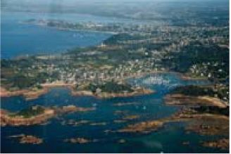
Uss et al.: Image informative maps for component-wise estimating parameters. . .

                                        Fig. 5 Nikon D80 noise variance dependence on image intensity for red, green, and blue channels.

                            Table 1 Sensor noise parameters for the Nikon D80 digital SLR camera (statistical error at one sigma level is specified)

                Component                                     c 0 (σ 2n:SI )                                c 1 (σ 2n:SD )                                      c2

                Red (calibration)                          7.6876  0.0373                        0.1460  7.03 × 10⁻⁴                           0.696 × 10⁻⁵  0.0485 × 10⁻⁵

                Red (NI þ DCT)                             8.5707  0.1145                        0.1412  10.04 × 10⁻⁴                          1.012 × 10⁻⁵  0.1300 × 10⁻⁵

                Green (calibration)                        5.0834  0.0473                        0.1352  7.03 × 10⁻⁴                           0.704 × 10⁻⁵  0.0492 × 10⁻⁵

                Green (NI þ DCT)                           6.4340  0.4337                        0.1270  16.45 × 10⁻⁴                          0.759 × 10⁻⁵  0.1030 × 10⁻⁵

                Blue (calibration)                        12.3381  0.0799                        0.1709  10.46 × 10⁻⁴                          2.387 × 10⁻⁵  0.0755 × 10⁻⁵

                Blue (NI þ DCT)                           13.0143  0.2064                        0.1702  12.48 × 10⁻⁴                          2.601 × 10⁻⁵  0.1110 × 10⁻⁵

                    We will first prove that estimation results obtained by the                     the noise in the Nikon D80 images does not strictly follow
                NI þ DCT method agree with the calibration data shown                               this linear model. Therefore, in order to nullify quadratic
                above. For this goal, we applied the NI þ DCT method to                             term c2 before estimation, we normalized the image intensity
                all images from the NED2012 database simultaneously by                              in each SW ISW by
                processing 1,500 SWs of 9 × 9 pixels randomly selected                                                              sffiffiffiffiffiffiffiffiffiffiffiffiffiffiffiffiffiffiffiffiffiffiffiffiffiffiffiffiffiffiffiffiffiffiffiffiffiffiffiffiffiffi
                from each NED2012 image (a total of 1; 500 × 25 ¼                                                                             c0 þ c1 Ī SW
                37; 500 windows). In this manner, very high estimation accu-                           ISW ¼ Ī SW þ ðISW − Ī SW Þ                                          ; (13)
                                                                                                                                     c0 þ c1 Ī SW þ c2 Ī 2SW
                racy of the c0 , c1 , and c2 coefficients can be reached.
                Estimation results for all three channels are shown in
                                                                                                    where Ī SW is the mean of ISW and c0 , c1 , and c2 are taken
                Table 1 (the NI þ DCT line). Figure 7 illustrates these results
                                                                                                    from Table 1. After such normalization, noise parameters
                for the blue channel.
                                                                                                    become as specified in Table 1, with c2 ¼ 0.
                    One can clearly see that there is no statistically significant
                difference between estimates of noise parameters obtained
                for two different datasets (the NED2012 database and the                            4.2 Accuracy Analysis of Signal-Dependent Noise
                set of 17 calibration images) by the calibration procedure                                Parameter Estimation
                and the NI þ DCT method (they differ by less than 4σ). It                           The considered set of four estimators, NI þ fBm, NI þ DCT,
                is worth noting that the accuracy provided by the                                   ASRPFR, and ClipPoisGaus_stdEst2D, were applied to each
                NI þ DCT method is only slightly worse than the one                                 of the 25 images of the NED2012 database in a component-
                obtained by the calibration procedure. In this test, the NI þ                       wise manner (red, green, and blue components were proc-
                DCT method shows its potential ability to deal with signal-                         essed independently). A SW of 9 × 9 pixels in size was
                dependent noise that is more complex than mixtures of addi-                         selected for both NI þ DCT and NI þ fBm. The choice of
                tive and Poisson/multiplicative noises.                                             this particular SW size is justified in this subsection. For
                    In the next experiment, we restricted ourselves to the case                     each component, the two noise variance components σ^ 2n:SI
                of a mixture of signal-independent and Poisson-like signal-                         and σ^ 2n:SD were estimated. Overall, 25 estimates were
                dependent noises. The overall noise variance is thus signal-                        obtained for each channel. Their empirical probability den-
                dependent: σ 2n ðIÞ ¼ σ 2n:SI þ I ⋅ σ 2n:SD . As was shown above,                   sity functions (pdfs), pdf (σ^ 2n:SI ) and pdf (σ^ 2n:SD ), are shown in

                Journal of Electronic Imaging                                              013019-9                                                   Jan–Mar 2013/Vol. 22(1)

Downloaded From: https://www.spiedigitallibrary.org/journals/Journal-of-Electronic-Imaging on 10 Jun 2022
Terms of Use: https://www.spiedigitallibrary.org/terms-of-use
Uss et al.: Image informative maps for component-wise estimating parameters. . .
1 2 3 4 5
6 7 8 9 10
11 12 13 14 15
16 17 18 19 20
21 22 23 24 25
Fig. 6 Images of the NED2012 database.
Fig. 7 Comparison of NI þ DCT and calibration noise variance estimates for the blue channel of the NED2012 database.
Figs. 8 and 9, respectively. The main statistical characteris- ClipPoisGaus_stdEst2D estimators is the significant number
tics of these estimates [mean Mð⋅Þ, bias and standard of outliers. However, they form a pronounced mode in the
deviation STDð⋅Þ] are given in Table 2. The bias measure vicinity of the true value of signal-independent and -depen-
is calculated as bias ¼ 100%½MðaÞ ^ − a0 ∕a0 , where a0 is dent noise component variances anyway. Therefore, we have
the true value of a. decided to characterize the performance of these estimators
Preliminary conclusions can be drawn from these by calling on extra robust measures. Specifically, median is
results. Among these four estimators, ASRPFR and used instead of mean value, and median absolute deviation
ClipPoisGaus_stdEst2D provide worse performance than (MAD) instead of standard deviation.
the NI þ fBm and NI þ DCT with regard to both signal- Estimates of signal-independent noise component vari-
independent and -dependent components. The main factor ance are biased for all four estimators. The absolute value of
that degraded the performance of the ASRPFR and the bias is the smallest for the NI þ DCT and NI þ fBm
Journal of Electronic Imaging 013019-10 Jan–Mar 2013/Vol. 22(1)
Downloaded From: https://www.spiedigitallibrary.org/journals/Journal-of-Electronic-Imaging on 10 Jun 2022
Terms of Use: https://www.spiedigitallibrary.org/terms-of-useUss et al.: Image informative maps for component-wise estimating parameters. . .
Fig. 8 Experimental pdfs of signal-independent noise component variance σ^ 2n:SI estimates by (a) NI þ fBm, (b) NI þ DCT, (c) ASRPFR, and
(d) ClipPoisGaus_stdEst2D. Calibration variances σ 2n:SI.0 are marked by vertical dot-dashed lines.
methods (i.e., less than 6%). It increases to more than 30% on Hurst exponent estimation. A second possible reason
for the ASRPFR method and to more than 12% for the could be deviations of real image texture from the assumed
ClipPoisGaus_stdEst2D. The estimates of the signal-depen- fBm-model.
dent noise component variance are practically unbiased for It is important to mention here that both ASRPFR and
the NI þ DCT method, negatively biased by about 6% for ClipPoisGaus_stdEst2D have been applied to NED2012
the NI+fBm method, and exhibit a positive bias less than images without normalization [Eq. (13)] for quadratic
25% for the ASRPFR and ClipPoisGaus_stdEst2D methods. term c2 compensation. The reason for this is that such nor-
It is worth highlighting that the NI þ DCT method pro- malization operates at the SW level and depends on image
vides the best estimation accuracy on both signal-indepen- partitioning during processing. We had no opportunity to
dent and -dependent components. More precisely, with modify the original implementation of ASRPFR and
regard to the standard deviation of the noise variance esti- ClipPoisGaus_stdEst2D to take this into account. There-
mates (specified in Table 2), it outperforms the NI þ fBm fore, in an additional experiment, we quantified the noncom-
method by approximately 1.25 to 2.6 times, the ASRPFR pensated c2 term influence on NI þ DCT (Table 2).
method by 3.6 to 10 times, and by an even greater degree Overall, it led to negative bias of signal-independent compo-
for the ClipPoisGaus_stdEst2D. We explain the reduced nent variance and positive bias of signal-dependent
performance of the NI þ fBm estimator with regard to the component variance. For red and green channels, this
NI þ DCT one by the sensitivity of the former to errors additional bias was negligible and does not exceed 5% in
Journal of Electronic Imaging 013019-11 Jan–Mar 2013/Vol. 22(1)
Downloaded From: https://www.spiedigitallibrary.org/journals/Journal-of-Electronic-Imaging on 10 Jun 2022
Terms of Use: https://www.spiedigitallibrary.org/terms-of-useUss et al.: Image informative maps for component-wise estimating parameters. . .
Fig. 9 Experimental pdfs of signal-dependent noise component variance σ^ 2n:SD estimates by (a) NI þ fBm, (b) NI þ DCT, (c) ASRPFR, and
(d) ClipPoisGaus_stdEst2D. Calibration variances σ 2n:SD.0 are marked by vertical dot-dashed lines.
magnitude. For the blue channel, this bias was more increase in the potential estimation accuracy for signal-inde-
significant, with a magnitude of about 15%. We thus believe pendent and -dependent noise components to about 2 and
this is evidence that the noncompensated c2 term can- 8 × 10⁻³ , respectively.
not explain the decreased performance of ASRPFR and Let us now assess the efficiency of the analyzed estima-
ClipPoisGaus_stdEst2D. tors with regard to the diagonal terms ðσ 2σ n:SI ; σ 2σ n:SD Þ of the
In Fig. 10, we detail the signal-independent and -depen- correlation matrix σ2c of coefficient vector c defined above
dent noise variance estimates obtained with the best NIþ by Eq. (12). For this purpose, two normalized errors, one
DCT estimator on each component (red, green, and blue) for σ^ 2n:SI and another one for σ^ 2n:SD, respectively, are to be
of all images from the NED2012 database. For most of considered:
the images, very accurate estimates were obtained. For
these images, the potential estimation accuracy on the sig- σ^ 2n:SI:norm ¼ ðσ^ 2n:SI − σ 2n:SI.0 Þ∕σ σn:SI and
nal-independent noise component variance is about 0.2–1, σ^ 2n:SD:norm ¼ ðσ^ 2n:SD − σ 2n:SD.0 Þ∕σ σ n:SD :
and it is about 0.8 − 2.2 · 10−3 on the signal-independent
noise component variance. But for some of the images, Note that for an efficient estimator, both σ^ 2n:SI:norm
namely 13, 15, 16, 22, and 23, an increased estimation and σ^ 2n:SD:norm should be distributed close to the normal dis-
error was observed. This is reflected by a corresponding tribution Nð0; 1Þ. The statistical efficiency of the analyzed
Journal of Electronic Imaging 013019-12 Jan–Mar 2013/Vol. 22(1)
Downloaded From: https://www.spiedigitallibrary.org/journals/Journal-of-Electronic-Imaging on 10 Jun 2022
Terms of Use: https://www.spiedigitallibrary.org/terms-of-useUss et al.: Image informative maps for component-wise estimating parameters. . .
Table 2 Mean value Mð·Þ, bias and standard deviation STDð·Þ of noise variance estimates on the NED2012 database.
(a) Signal-independent component
Estimator Component σ 2n:SI.0 M σ^ 2n:SI Bias, % STDσ^ 2n:SI
NI þ fBm (N ¼ 9 Red 7.94 7.60 −4.32 2.69
Green 5.06 5.06 −0.04 8.99
Blue 11.36 11.70 2.99 5.42
NI þ DCT (N ¼ 9) Red 7.94 8.08 1.80 1.33
Green 5.06 5.16 1.88 3.46
Blue 11.36 12.05 6.14 3.02
NI þ DCT (without quadratic Red 7.94 7.84 −1.22 1.33
term correction)
Green 5.06 4.97 −1.60 3.91
Blue 11.36 10.99 −3.17 2.24
ASRPFR Red 7.94 10.51 (median) 32.37 7.53 (MAD)
Green 5.06 31.11 (median) 514.77 31.11 (MAD)
Blue 11.36 25.52 (median) 124.72 14.09 (MAD)
ClipPoisGaus_stdEst2D Red 7.94 10.60 (median) 37.83 13.09 (MAD)
Green 5.06 11.51 (median) 126.35 59.10 (MAD)
Blue 11.36 13.83 (median) 12.13 10.62 (MAD)
(b) Signal-dependent component
Estimator Component σ 2n:SD.0 M σ^ 2n:SD Bias, % STDσ^ 2n:SD
NI þ fBm (N ¼ 9) Red 0.142 0.133 −6.855 0.016
Green 0.134 0.124 −7.869 0.017
Blue 0.174 0.162 −6.937 0.015
NI þ DCT (N ¼ 9) Red 0.142 0.143 0.834 0.008
Green 0.134 0.134 −1.748 0.014
Blue 0.174 0.173 −1.164 0.010
NI þ DCT (without quadratic Red 0.142 0.149 4.550 0.010
term correction)
Green 0.134 0.140 4.421 0.015
Blue 0.174 0.199 12.360 0.013
ASRPFR Red 0.142 0.153 (median) 7.429 0.031 (MAD)
Green 0.134 0.138 (median) 2.831 0.079 (MAD)
Blue 0.174 0.216 (median) 24.135 0.047 (MAD)
ClipPoisGaus_stdEst2D Red 0.142 0.148 (median) 1.100 0.052 (MAD)
Green 0.134 0.138 (median) 2.135 0.170 (MAD)
Blue 0.174 0.195 (median) 14.210 0.062 (MAD)
Bold values indicates values with the lowest bias magnitude and STD.
Journal of Electronic Imaging 013019-13 Jan–Mar 2013/Vol. 22(1)
Downloaded From: https://www.spiedigitallibrary.org/journals/Journal-of-Electronic-Imaging on 10 Jun 2022
Terms of Use: https://www.spiedigitallibrary.org/terms-of-useUss et al.: Image informative maps for component-wise estimating parameters. . .
Fig. 10 (a) Signal-independent and (b) signal-dependent noise component variance according to image index i NED estimated by the NI þ DCT on
red, green, and blue components of each image from the NED2012 database. The true noise parameters are shown as dashed horizontal lines.
estimators with regard to these bounds can be estim- As is shown, the NI þ DCT estimator exhibits rather high
ated as efficiency for different SW sizes, with a value of about 10 for
both noise components. Note that for the NI þ fBm estima-
X
Ne tor, the corresponding efficiency (not included in Table 3) is
e^ ¼ 100% ⋅ N e ∕ σ^ 2norm:XX:i ; (14) about 2%, and it is less than 0.1% for both the ASRPFR and
i¼1 ClipPoisGaus_stdEst2D estimators. More detailed analysis
shows that the performance of the NI þ DCT estimator is
where XX is the noise component label (either SI or SD), and highest for N ¼ 9 and 11. It is slightly degrading for
the sum for each estimator is calculated in Eq. (14) over all N ¼ 13 and the degradation is much more significant for
N e ¼ 75 available estimates. N ¼ 7. This can be explained by the influence of two factors
Figure 11 displays σ^ 2n:SI:norm and σ^ 2n:SD:norm pdfs, respec- compensating each other. On one side, the accuracy of tex-
tively, for the best NI þ DCT method (with N ¼ 9). The ture parameter estimation reduces for smaller sized SWs.
theoretical pdf Nð0; 1Þ is added for comparison purposes. This factor is responsible for the decline in performance
Efficiencies e^ for both noise components are shown in for N ¼ 7. On the other hand, the image texture becomes
Table 3 for four different window sizes: N ¼ 7, 9, 11, more heterogeneous for larger windows, making the fBm
and 13. model less adequate. This factor is responsible for the slight
Fig. 11 Empirical pdfs of the normalized estimates of signal-independent and signal-dependent noise components variances by the NI þ DCT
estimator N ¼ 9. The theoretical pdf Nð0; 1Þ is shown as a dashed black curve.
Journal of Electronic Imaging 013019-14 Jan–Mar 2013/Vol. 22(1)
Downloaded From: https://www.spiedigitallibrary.org/journals/Journal-of-Electronic-Imaging on 10 Jun 2022
Terms of Use: https://www.spiedigitallibrary.org/terms-of-useYou can also read