How Many Reindeer? UAV Surveys as an Alternative to Helicopter or Ground Surveys for Estimating Population Abundance in Open Landscapes
←
→
Page content transcription
If your browser does not render page correctly, please read the page content below
Article

How Many Reindeer? UAV Surveys as an Alternative to
Helicopter or Ground Surveys for Estimating Population
Abundance in Open Landscapes
Ingrid Marie Garfelt Paulsen 1,*,†, Åshild Ønvik Pedersen 1,†, Richard Hann 2, Marie-Anne Blanchet 1,
Isabell Eischeid 1,3, Charlotte van Hazendonk 4, Virve Tuulia Ravolainen 1, Audun Stien 3 and
Mathilde Le Moullec 5

                                              1 Norwegian Polar Institute, Fram Centre, 9296 Tromsø, Norway
                                              2 Department of Engineering Cybernetics, Norwegian University of Science and Technology,
                                                7491 Trondheim, Norway
                                              3 Department of Arctic and Marine Biology, UiT—The Arctic University of Norway, 9037 Tromsø, Norway

                                              4 Department of Arctic Geophysics, University Centre in Svalbard (UNIS), 9171 Longyearbyen, Norway

                                              5 Centre for Biodiversity Dynamics, Department of Biology, Norwegian University of Science and

                                                Technology, 7491 Trondheim, Norway
                                              * Correspondence: ingrid.paulsen@npolar.no; Tel.: +47-96-91-36-86
                                              † These authors contributed equally to this work.

                                              Abstract: Conservation of wildlife depends on precise and unbiased knowledge on the abundance
                                              and distribution of species. It is challenging to choose appropriate methods to obtain a sufficiently
                                              high detectability and spatial coverage matching the species characteristics and spatiotemporal use
                                              of the landscape. In remote regions, such as in the Arctic, monitoring efforts are often resource-
                                              intensive and there is a need for cheap and precise alternative methods. Here, we compare an un-
Citation: Paulsen, I.M.G.; Pedersen,          crewed aerial vehicle (UAV; quadcopter) pilot survey of the non-gregarious Svalbard reindeer to
Å.Ø.; Hann, R.; Blanchet, M.-A.;              traditional population abundance surveys from ground and helicopter to investigate whether UAVs
Eischeid, I.; van Hazendonk, C.;              can be an efficient alternative technology. We found that the UAV survey underestimated reindeer
Ravolainen, V.T.; Stien, A.; Le               abundance compared to the traditional abundance surveys when used at management relevant spa-
Moullec, M. How Many Reindeer?                tial scales. Observer variation in reindeer detection on UAV imagery was influenced by the RGB
UAV Surveys as an Alternative to              greenness index and mean blue channel. In future studies, we suggest testing long-range fixed-wing
Helicopter or Ground Surveys for
                                              UAVs to increase the sample size of reindeer and area coverage and incorporate detection proba-
Estimating Population Abundance
                                              bility in animal density models from UAV imagery. In addition, we encourage focus on more effi-
in Open Landscapes. Remote Sens.
                                              cient post-processing techniques, including automatic animal object identification with machine
2023, 14, 9. https://doi.org/
                                              learning and analytical methods that account for uncertainties.
10.3390/rs15010009

Academic Editor: Niki Liu                     Keywords: aaerial survey; animal detection; distance sampling; helicopter; monitoring;
Received: 10 October 2022                     strip transect; Svalbard; total count; ungulate
Revised: 13 December 2022
Accepted:13 December 2022
Published: 20 December 2022
                                              1. Introduction
                                                   The distribution and abundance of species are key parameters for conservation and
                                              management of wildlife [1]. Yet, it remains challenging to estimate population size with
Copyright: © 2022 by the author.
Licensee MDPI, Basel, Switzerland.
                                              high precision and low bias (i.e., accuracy [2]) at relevant spatial scales [3]. There are nu-
This article is an open access article
                                              merous methods to estimate wildlife abundance and density—ranging from direct popu-
distributed   under    the      terms   and   lation counts to population indices proportional to the true population size [4,5]. Abun-
conditions of the Creative Commons            dant and easily detectable species are commonly monitored with direct density estima-
Attribution      (CC      BY)       license   tion methods, which includes complete or partial census, strip transect, distance sampling
(https://creativecommons.org/licenses/        or capture-recapture programs [5,6]. Recent developments in uncrewed aerial vehicles
by/4.0/).                                     (UAVs) technology open new opportunities to survey animal populations as a

Remote Sens. 2023, 15, 9. https://doi.org/10.3390/rs15010009                                                   www.mdpi.com/journal/remotesensing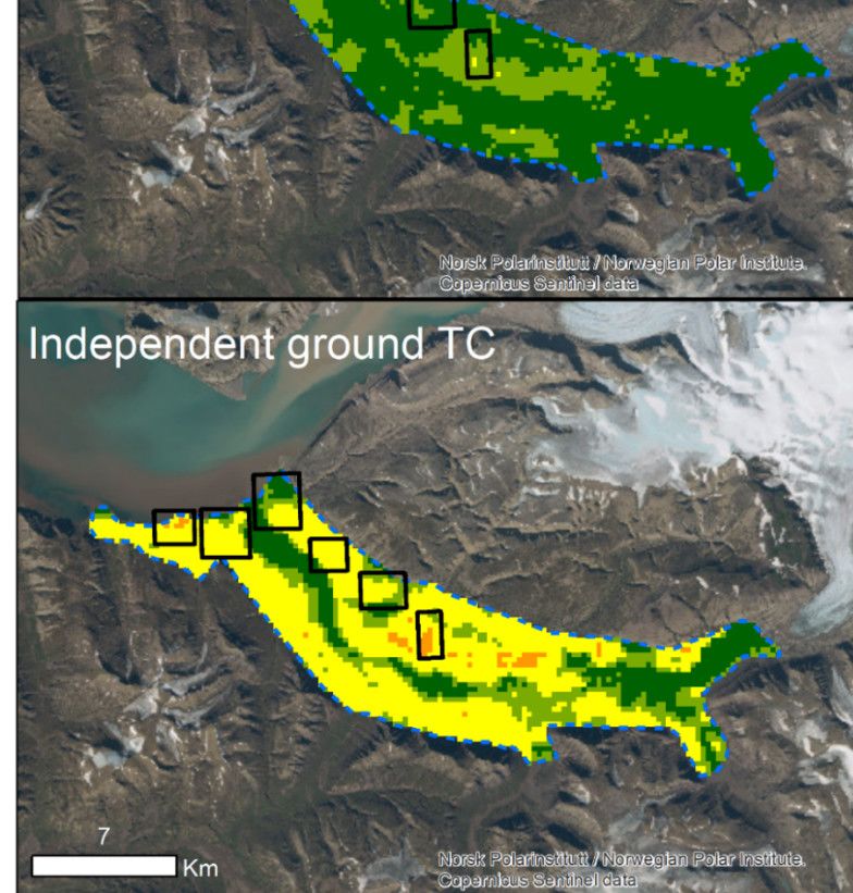
Remote Sens. 2023, 15, 9                                                                                             2 of 24

                           replacement or supplement to traditional survey techniques [7]. UAVs offer several ad-
                           vantages compared to traditional aerial or ground surveys (e.g., cost effectiveness, re-
                           duced environmental impact and disturbance, and operational range [8,9]), however,
                           whether UAV methods have improved accuracy and are more efficient than traditional
                           survey methods is largely unknown (but see [10,11]).
                                 Remote wildlife populations are traditionally counted on foot or using aerial surveys
                           from helicopters or planes depending on the species characteristics and management area
                           of interest [5,12-15]. Aerial surveys are costly, with a high carbon footprint, and they are
                           challenging when it comes to detectability and uncertainty estimates [16-19]. In compari-
                           son, counting on foot along a survey line is more time-consuming and can be logistically
                           difficult in remote areas, with terrain features (e.g., river, cliffs) or, e.g., when the species
                           is sparsely distributed. Distance sampling is a common method that can assess uncertainty
                           in abundance surveys along such line transects [4,20]. A key assumption is that the prob-
                           ability of detecting an animal decreases with increasing distance from the observer. There-
                           after, abundance estimates account for detection probability. Total count is a method as-
                           suming that all animals are counted without error. When conducted in a well-delimited
                           area with information on presence/absence in sub-units, uncertainty can still be evaluated
                           [21]. Both methodologies can be used to predict densities across larger areas [22]. For an
                           aerial survey recording, e.g., images along a fixed transect width (i.e., strip transect from
                           crewed aircraft or UAV flying at constant height), detection is independent of distance
                           from the transect line. Yet, there are other factors that can influence detection of an object,
                           such as the image quality and resolution [15]. Integrating measures of detection error
                           within a surveyed area and identifying habitat covariates strongly correlated with the
                           population density can greatly improve the accuracy of estimates when extrapolating den-
                           sity to larger spatial scales [3]. Only in the last decade, UAVs have been tested and suc-
                           cessfully applied as a cost-effective alternative to traditional surveys to estimate abun-
                           dance of wildlife, especially in gregarious species [23,24], but also for solitary animals
                           [9,25].
                                 In the High Arctic remote Svalbard archipelago, the wild Svalbard reindeer Rangifer
                           tarandus platyrhynchus, is the largest resident mammalian herbivore in the terrestrial tun-
                           dra ecosystem [26]. Svalbard reindeer are non-gregarious, inhabiting open landscapes and
                           can appear in high density (>10 individuals/km2). The reindeer is subject to long-term
                           monitoring because it is a key-species impacting tundra vegetation [27], is harvested lo-
                           cally by recreational hunting [28] and is sensitive to climate change [29,30]. The long-term
                           monitoring is relying on total population counts along fixed routes on foot [21,31] or by
                           helicopter [32,33], and capture-mark-recapture techniques (see [34]). Lately, there has
                           been focus on quality assurance and standardisation of monitoring methods of the long-
                           term ground total counts with distance sampling [21]. Total counts were found unbiased
                           when compared to resighting of marked reindeer and highly precise when repeating
                           counts. In comparison, distance sampling was also unbiased, while precision was lower
                           than total counts, according to the number of transects and groups detected. This has en-
                           abled range-wide monitoring of Svalbard reindeer using the most appropriate methodol-
                           ogy according to terrain characteristics [22]. Both total counts and distance sampling esti-
                           mated similar abundances across Svalbard (22,615 ± 401 [± SE] and 21,079 ± 2983, respec-
                           tively) and found that abundance was strongly correlated with vegetation productivity
                           [22]. Thus, both ground total counts and distance sampling can serve as reference abun-
                           dance estimates to evaluate other methodologies. Local wildlife managers (the Governor
                           of Svalbard) have, however, annually monitored reindeer since 1998 in hunting units by
                           total counts from helicopter, and the accuracy of these counts remain to be evaluated
                           [32,35]. In addition, there is a desire for development of monitoring methods that reduce
                           disturbance and lower human footprints [36], which suggests the use of UAVs [37].
                                 In this paper, we assess the precision and detection rate of reindeer abundance from
                           a UAV pilot survey compared to traditional ground and helicopter surveys. We compare
                           the survey methods in the same spatial extent by developing models of estimated reindeer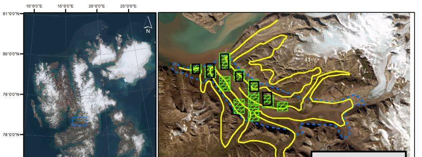
Remote Sens. 2023, 15, 9                                                                                               3 of 24

                           abundance and predicting the models over the same sampling scales using correlated hab-
                           itat covariates. We test the feasibility of collecting data on reindeer abundance and varia-
                           bles affecting detection probability using UAVs, and investigate potential problems and
                           pitfalls associated with aerial monitoring compared to ground-based surveys.

                           2. Materials and Methods
                           2.1. Study Area and Species
                                The Arctic Svalbard archipelago (74–81°N, 15–30°E), Norway, measures around
                           62,700 km2, with approximately 60% covered by glaciers, 25% by barren rocks and only
                           15% by vegetation [38]. We conducted the study in Sassendalen, one of the largest valleys
                           in Central Spitsbergen (Figure 1). The valley is surrounded by peaks up to 1200 m.a.s.l.
                           and dominated by a large river and continuous vegetation cover with wetland, ridges,
                           and heath present only in the valley bottoms and on the lower parts of the mountain
                           slopes (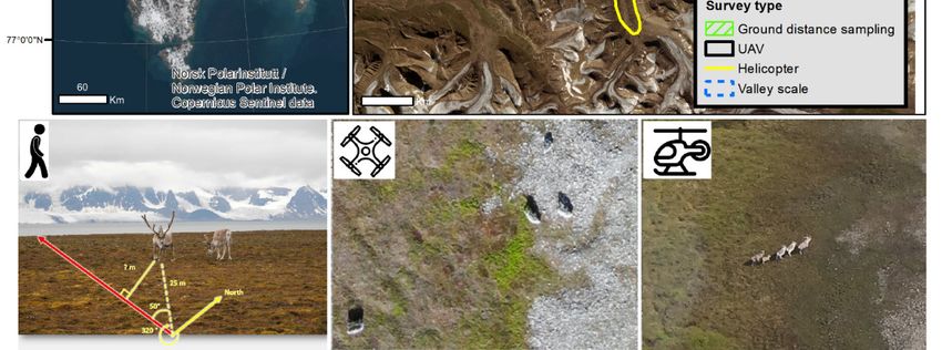
Remote Sens. 2023, 15, 9 4 of 24
and mortality rates, and thus abundances [29]. This led us to assume similar population
dynamics and thereby densities between the adjacent valleys.
2.2. Field Data Collection
Reindeer data were collected by four survey methodologies: (1) Ground-based dis-
tance sampling (hereafter ‘ground DS’), which served as reference to assess accuracy of
the other methods, (2) UAV strip transects, (3) helicopter total counts and, (4) ground total
counts from the neighbouring valley (hereafter ‘independent ground TC’) to test if extrap-
olations can replace the need for aerial surveys (i.e., helicopter and UAV). See Figure 2 for
an illustration of the workflow.
Figure 2. Visualisation of the workflow, including field survey design, postprocessing and data
analysis of the four survey methods ground distance sampling (ground DS), UAV, helicopter, and
independent ground total counts (independent ground TC).
The UAV and DS surveys were conducted on the same transects (see below) during
14–17 July 2021, but 1 day apart to reduce potential disturbance of reindeer by observers.
The helicopter survey was conducted one week prior to the UAV and DS surveys (6 July)
and was part of an annual census of reindeer in the valleys on Nordenskiöld Land by the
Governor of Svalbard (Figure 1). Because the helicopter survey lacked positional infor-
mation of individual reindeer, but densities and spatial distribution of reindeer in neigh-
boring valleys are expected to be similar, we used the independent ground TC from the
adjacent valley (Appendix A), conducted during 30 June–7 July 2021.
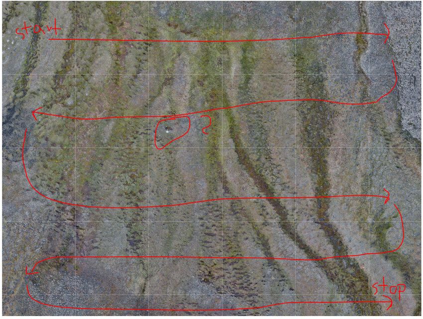
2.2.1. Ground Distance Sampling Survey
We followed the DS survey protocols described by [21,22] for estimating abundance
of Svalbard reindeer. We allocated 10 transect lines in north–south direction, from the
mountain foothills to the riverbanks, on each side of the main river in Sassendalen (Figure
1). We chose one random latitude for the first line and placed additional parallel transect
lines systematically apart 2.5 km east or west from this latitude to avoid overlapping rein-
deer observations and to avoid violation of the assumption of independence [20]. We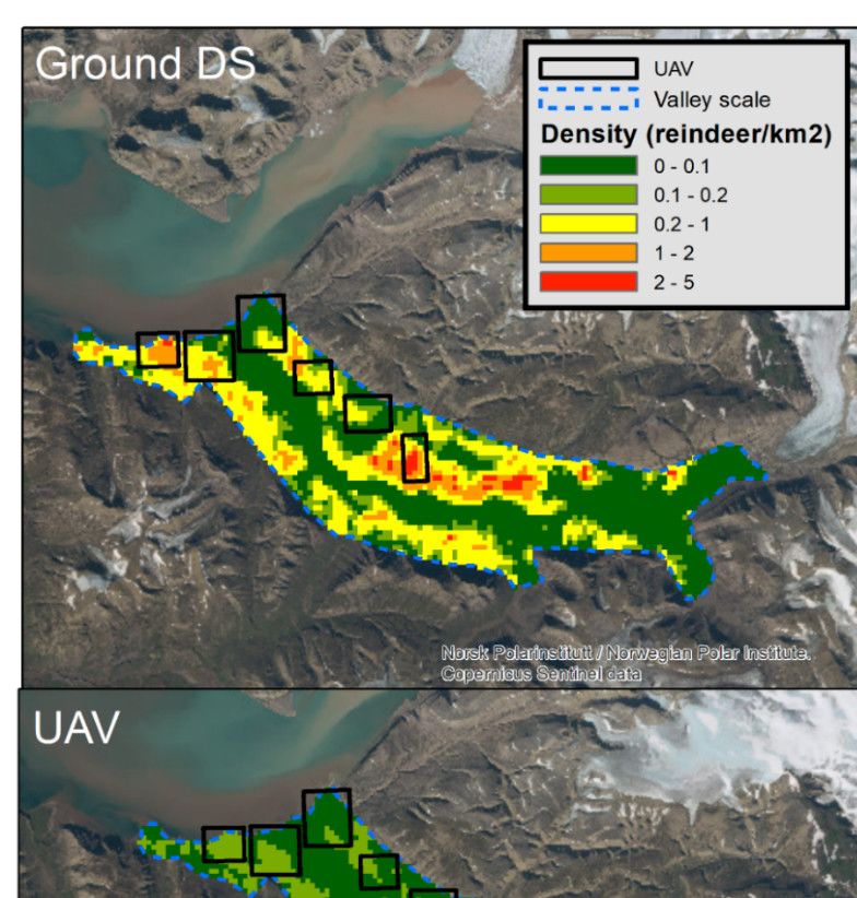
Remote Sens. 2023, 15, 9                                                                                         5 of 24

                           chose this systematic orientation across the valley (i.e., river bed to mountain side or vice
                           versa) to reduce any bias from potential gradients in animal density related to, e.g., plant
                           phenology and/or habitat configuration [45]. The length of each transect varied depending
                           on the length from the mountain side to the riverbank (1.2 km to 2.9 km). All transects
                           were walked by one observer (the same main observer as in [21,22]) at a constant speed
                           (2–3 km h−1) without stopping, except during measurements. A handheld GPS and a com-
                           pass were used to keep the line direction, and single reindeer or clusters were detected on
                           both sides of the transect line with the naked eye. To follow the assumption of constant
                           detection along the transect line, no scanning for reindeer was done when stopping to take
                           measurements. Each observation was measured by laser binoculars (10 × 42 Leica Geovid,
                           Wetzlar, Germania) to the nearest metre and a compass was used to measure the angle
                           from the observer to the reindeer (Figure 1). For practical reasons when using the laser,
                           measurements were taken to the largest reindeer (e.g., a mother rather than her calf) or
                           the middle individual of a group of adults. The geographic position of the observer in the
                           transect was also recorded. The positions of reindeer individuals/groups and perpendic-
                           ular distances to the line were calculated and used in the final dataset.

                           2.2.2. UAV Survey
                                 Six out of the ten line transects were mapped by an off-the-shelf DJI Mavic 2 Enter-
                           prise drone, equipped with a zoomable (24–48 mm) RGB camera. Flight plans for each
                           line transect were prepared pre-flight with a commercial mapping software (DJIFlight-
                           Planner, ver. 2.13). The flight plans were flown automatically with flight altitude 110–120
                           m above ground with a nadir (downward-looking) orientation of the camera. Test flights
                           with different altitudes (e.g., 20–120 m) were performed before the survey to verify that
                           reindeer could be detected on images at that height and to ensure that reindeer were min-
                           imally disturbed. At this altitude, the widest field of view (i.e., 24 mm) was used, giving
                           a theoretical ground sample distance (GSD) of 4.4 cm and a swath width of 174 m. Side
                           overlap was chosen with 65% and the nominal forward overlap with 85%. All lines had a
                           run separation of 61 m and ran in an east–west direction. Ground speed was set to maxi-
                           mum 30 km/h and pictures taken with a frame rate of 2 s. The camera settings were on
                           auto, but it was ensured that the shutter speed would not exceed 1/200 to prevent motion
                           blur (max. shutter speed = GSD/ground speed), otherwise flight velocity was reduced. The
                           total mapped area width covered 500 m on each side of the transect line. The total length
                           of the mapping flight lines was between 20–40 km and typically took between 2–4 batter-
                           ies to cover.

                           2.2.3. Helicopter Survey
                                 Reindeer were counted by four observers (two pilots and two observers) in a Super
                           Puma helicopter flying 60–100 metres above the ground according to protocols by the
                           Governor of Svalbard [32]. The flight paths (Figure 1) were assumed to cover the most
                           important reindeer summer habitats in the Sassendalen hunting unit (see for a map of
                           hunting units). The spatial extent of the helicopter surveyed area was defined as the entire
                           flat valley bottom of Sassendalen and a buffer of 1 km (500 m on either side of the heli-
                           copter) around the flight routes (216 km). The census provides a single total count of all
                           the individuals encountered, classified as calf, female/young and male, without any infor-
                           mation on location of each animal.

                           2.2.4. Independent Total Counts Survey
                                Total counts followed the protocols described by [21,22] and were conducted in Ad-
                           ventdalen, the neighboring valley. Five observers walked separate predefined routes (~1
                           km apart from each other), scanning the entire area with 10 × 42 mm binoculars for rein-
                           deer. During the count, reindeer were categorised by age as calves, yearlings, or adults
                           (≥2 years old) based on body size and antler characteristics. The geographic position of
Remote Sens. 2023, 15, 9                                                                                         6 of 24

                           individual reindeer or groups were noted. At this time of the year, reindeer still have parts
                           of their winter fur, making them conspicuous against the open tundra landscape.

                           2.3. Data Analyses
                                 We estimated reindeer abundance based on field data from the survey methods of
                           ground DS, UAV, and independent ground TC, as detailed below. Note that the helicopter
                           total count was a single value with no data analysis. To compare estimates, we developed
                           density spatial models (DSM) for each method as a function of vegetation productivity
                           (Figure 2). Reindeer densities in summer correlate with vegetation productivity, as ex-
                           pressed by the vegetation productivity index ‘maximum normalised difference vegetation
                           index’ (maxNDVI) [22,46]. Due to this relationship, maxNDVI was used as the common
                           denominator to project the DSMs onto the same spatial extents in this study. The vegeta-
                           tion productivity layer was calculated by averaging the maxNDVI values from MODIS-
                           satellites (Jacksonville, FL, USA) for the last five years (2017–2021) and then resampled to
                           resolution 240 × 240 m. We used average maxNDVI because cloud coverage and random
                           variation can affect the timing of NDVI contributing to high between-year variation
                           [47,48]. The statistical models were adapted from Le Moullec et al. [21,22]. We fitted all
                           models in R version 1.4.1717 [49].

                           2.3.1. Ground Distance Sampling DSM
                                The ground DS consisted of a two-stage approach with a detection probability esti-
                           mation and a DSM accounting for the imperfect detection [20]. To prepare the data, we
                           divided the transect lines into smaller segments and summarised count data and
                           maxNDVI per segment, as recommended by Miller et al. [50]. We divided the transects
                           into equal lengths of 500 m (for effect of segment lengths on model output, see Table S1
                           in Le Moullec et al. [22]) and truncated the transect width to 95 % of all distances rounding
                           up to the nearest reindeer group. We modelled detection probability using half-normal
                           and hazard-rate functions and determined the top ranked model using AIC. We used the
                           standard distance sampling functions ‘ds’, ‘dsm’ in the packages Distance and dsm, re-
                           spectively. We included weather (sunny or cloudy) as a covariate because this variable
                           was the main covariate influencing detection in Le Moullec et al. [22]. The hazard rate
                           function with weather as a covariate had the lowest AIC and was therefore selected for
                           the density function (Appendix B). We used the most parsimonious density model from
                           Le Moullec et al. [22], which modelled individuals per segment as a function of maxNDVI,
                           using a log-link quasi-Poisson model. The final model was fitted using the restricted max-
                           imum likelihood (REML) framework and residuals were checked for normality, auto-cor-
                           relation, and goodness of fit (Table A3, Figure A3).

                           2.3.2. UAV DSM
                                The UAV survey generated many single images (n = 10,479) with considerable image
                           overlap. To reduce the number of images for reindeer counting, single images were pro-
                           cessed into orthomosaic images for each transect line using a structure from motion
                           method in Agisoft Metashape, ver. 1.7.2. The orthomosaic images were typically large (ca.
                           30,000 × 40,000 pixels covering areas between 1.5–3.4 km², GSD between 3.7–4.1 cm/pixel)
                           and were segmented into smaller tiles of 4000 × 3000 pixels with a 10% overlap to ensure
                           that animals on the border of the tiles could be identified. Observers (n = 6) manually
                           counted the number of reindeer inside each tile (see protocol in Appendix C). Positions
                           and image snapshots of detected reindeer were stored for each observer. In addition, raw
                           single images were counted by three observers to check if reindeer were lost from the
                           image or appeared twice in the processing steps because of reindeer movement. This re-
                           sulted in detection of four reindeer that appeared more than once, and these copies were
                           excluded. Further, all detected reindeer were scanned a third time by two observers and
                           assigned a certainty category (‘low’, ‘medium’, and ‘high’) according to how clear they
Remote Sens. 2023, 15, 9                                                                                        7 of 24

                           appeared on the image snapshot. Only reindeer that were assigned as ‘medium’ or ‘high’
                           were used in the final dataset to reduce the potential for confusing reindeer with, e.g., a
                           rock or another grey structure. We termed this dataset ‘confirmed’ reindeer. Furthermore,
                           we divided the area of the six UAV transects into grids with the same resolution as the
                           resampled maxNDVI layer (240 × 240 m) and summarised the number of confirmed rein-
                           deer per pixel.
                                 Based on the confirmed reindeer dataset, we fitted a hurdle model to avoid overdis-
                           persion from the high number of pixels with no reindeer observations. The hurdle model
                           deals with the response variable in two stages: (1) The presence/absence of reindeer in a
                           certain unit (i.e., pixel) and (2) a count model estimating how many reindeer were present
                           in that unit (when reindeer were present). The final hurdle model contained a zero-trun-
                           cated negative binomial distribution, assuming a logit-link function in both the pres-
                           ence/absence and the count model (Appendix D). We included maxNDVI as a covariate
                           in the presence-absence and count models. The analysis was done with the function ‘hur-
                           dle’ in the package pscl, and residuals were checked for normality, autocorrelation, and
                           goodness of fit.
                                 Since reindeer detection was imperfect among the seven observers, we explored what
                           could cause this variation. We tested if RGB image values (i.e., grey colored reindeer on
                           green vegetation would stand out more than on grey, barren, or non-vegetated terrain, or
                           if luminance (lower detection of reindeer on darker images) influenced observer detection
                           in the image. We extracted median luminance and mean red-green-blue (RGB) values
                           from each tiled image, and from the mean G and B values we calculated a color-based
                           vegetation index, here termed ‘Greenness Index’ (G-B [51,52]). We tested whether the
                           presence of reindeer in an image (from the ‘confirmed’ dataset) was detected or not by the
                           six observers and how the different covariates influenced this probability of detection. For
                           this, we used generalised linear mixed effect models (presence/absence model, binomial
                           family, ‘glmer’ function in the lme4 package) with the observer ID as random effects and
                           the image covariate of interest as fixed effect. In Appendix E, we also investigated factors
                           influencing the number of reindeer detected in an image, when at least one reindeer was
                           detected (counts model). These detection models influencing the reindeer presence/ab-
                           sence and counts reflect the two steps from the hurdle model.

                           2.3.3. Independent Total Counts DSM
                                 Given that reindeer densities are spatially synchronous and positively correlated
                           with maxNDVI, we projected a DSM built with data from the adjacent Adventdalen valley
                           ground TC into areas of Sassendalen. This allowed us, for instance, to evaluate corre-
                           spondence by checking if the actual abundance from the helicopter census in Sassendalen
                           fell within the standard error of these independent ground TC. Similarly, as in Le Moullec
                           et al. [33] and in the UAV density models described above, we modelled reindeer density
                           per pixel (240 × 240 m) with a hurdle model. We investigated this in two steps with a
                           presence/absence and count model as a function of the maxNDVI. Details on the proce-
                           dure are outlined in Appendix A.

                           2.4. Comparison of Survey Methods
                                To assess each survey method, we chose to predict each density model across: (1) The
                           ground DS covered area, (2) the UAV covered area, and (3) at an ecologically relevant
                           valley scale for management. Since the habitat characteristics and elevation ranges were
                           different for the helicopter surveyed area (0.6–601 m) than for the ground and UAV tran-
                           sect area (0.7–317 m), we did not predict the ground DS and UAV density models to the
                           helicopter surveyed area. Estimates were compared to the the ground DS and precisions
                           were compared with the coefficient of variation (CV, the ratio of the standard deviation
                           to the mean). Lower CV indicates higher precision.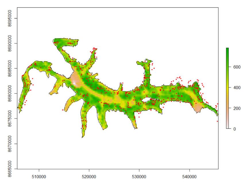
Remote Sens. 2023, 15, 9                                                                                                 8 of 24

                           3. Results
                           3.1. Field Survey Characteristics
                                The ground DS survey detected 50 groups of reindeer (n = 104 individuals, mean
                           group size = 2), walking 23.6 km on foot with a transect truncation width of 907 m (i.e.,
                           covering an area of 42.7 km2). The UAV survey, which covered about 40% of the same
                           transects (16.2 km2), detected 32 confirmed reindeer. The helicopter survey covered the
                           largest area (286.2 km2) and resulted in 1559 observed reindeer (Figure 1). The range in
                           vegetation productivity within the three sampling areas were similar (range for ground
                           DS [0.04–0.82], UAV [0.09–0.82] and helicopter [0.04–0.82]), with a mean maxNDVI of ap-
                           proximately 0.50.

                           3.2. Detection of Reindeer
                                The average detection probability for the ground DS survey was 0.40 ± 0.10 with 30%
                           of the reindeer clusters detected within approximately 500 m. Sunny weather conditions
                           resulted in higher reindeer detectability than cloudy (Figure A2). For the UAV survey, the
                           average detection rate of confirmed reindeer varied between observers by 46–70% (n = 6).
                           Variation of reindeer detection in the UAV imagery for the presence/absence model
                           showed an association with the greenness index and blue color channels when accounting
                           for observer variability (Figure 3). High values in the greenness index (i.e., greener vege-
                           tation ground cover) resulted in increased detectability, while high values of the blue
                           channel decreased detectability. In addition, all variables associated with darker ground,
                           except for the greenness index, decreased the probability to count the correct number of
                           reindeer in an image when at least one reindeer was present (Figure A7, Table A5).

                           Figure 3. Probability of an observer to detect the presence of a Svalbard reindeer known to be pre-
                           sent on a UAV image. Predicted estimates from linear mixed effect of presence/absence models (see
                           Table A5 for the model selection). (left) Variation in detection probability based on the greenness
                           index (G-B), (right) Variation in detection probability based on mean blue channel values. The figure
                           shows mean detection probability with 95 % confidence intervals (solid line and shaded area), indi-
                           vidual observer differences (stippled coloured lines), and observed covariate values (black points).

                           3.3. Reindeer Densities and Spatial Projections
                                 All three DSMs predicted a positive correlation between vegetation productivity
                           (maxNDVI) and reindeer densities (Figure 4). Reindeer density remained low until
                           around maxNDVI of 0.6–0.7 and thereafter increased steeply. However, the strength of
                           the relationship was markedly lower for UAV, while the ground DS and independent
                           total counts were similar (Figure 4).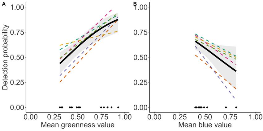
Remote Sens. 2023, 15, 9                                                                                                   9 of 24

                           Figure 4. Predicted density of Svalbard reindeer (number of animals per km2) based on data from
                           the three different survey methods (ground DS, drone, and independent total counts) as a function
                           of maximum normalised difference vegetation index (maxNDVI, i.e., proxy of biomass production).

                                 The independent total counts model from the neighboring valley estimated similar
                           abundances in the helicopter surveyed area (1515 ± 101, Table 1) as the helicopter survey
                           (n = 1559) in Sassendalen. The UAV density model estimated the lowest abundances with
                           the largest uncertainties (i.e., CVs range: 0.11–0.29), underestimating abundance by 70–75
                           % compared to ground DS and UAV at the different sampling scales. The ground DS and
                           the independent ground TC estimated similar abundance at all sampling scales. The in-
                           dependent ground TC gave the most precise estimates (CVs range: 0.07–0.24), while
                           ground DS precision was intermediate (CVs range: 0.22–0.26) (Table 1, Figure 5).

                           Table 1. Estimated Svalbard reindeer abundance ± SE in Sassendalen from density spatial models.
                           Predicted abundance for each density model at three scales; Ground distance sampling (DS) scale
                           (area covered by ground DS), UAV scale (area covered by UAV), the valley scale (ecologically rele-
                           vant management area), and helicopter scale (area covered by helicopter). See Figure 1 for delinea-
                           tion of study areas. Coefficient of variations (CV) are in parentheses. Because the habitat character-
                           istics and elevation ranges were different for the helicopter surveyed area (0.6–601 m) than for the
                           ground and UAV transect area (0.7–317 m), we did not predict the ground DS and UAV density
                           models to the helicopter surveyed area.

                                                                  Estimated Abundance
                                                    UAV       Ground DS                                         Helicopter
                                                                             Valley Scale
                              Survey Method    Sampling Area Sampling Area                                    Surveyed Area
                                                                              (161.7 km2)
                                                  (16.2 km2)    (42.7 km2)                                     (286.2 km2)
                                                   164 ± 43      351 ± 84      920 ± 202
                                Ground DS                                                                              -
                                                 (CV = 0.26)   (CV = 0.24)    (CV = 0.22)
                                                    32 ± 9        77 ± 15       243 ± 26
                                   UAV                                                                                 -
                                                 (CV = 0.29)   (CV = 0.19)    (CV = 0.11)
                                Helicopter             -             -             -                                1559 *
                            Independent ground     131 ± 32      311 ± 48       958 ± 82                          1515 ± 101
                                    TC           (CV = 0.24)   (CV = 0.15)    (CV = 0.09)                        (CV = 0.07)
                           * Actual reindeer number counted in the helicopter survey.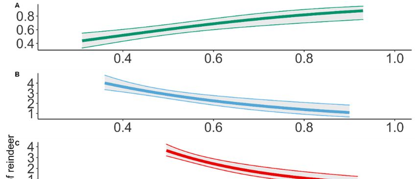
Remote Sens. 2023, 15, 9                                                                                             10 of 24

                           Figure 5. Predicted density (number of animals per km2) of Svalbard reindeer based on density spa-
                           tial models with maxNDVI as a covariate for the ground line transect distance sampling (upper),
                           UAV survey (middle) and independent total counts model from a neighboring valley at the valley
                           scale. The map shows predicted densities at the valley scale for pixel resolution of 240 × 240 m.

                           4. Discussion
                                 Our comparison of the different survey methods—ground DS, UAV, helicopter, and
                           independent ground TC surveys—for estimating Svalbard reindeer abundance and den-
                           sity showed that UAV imagery underestimated the number of reindeer as compared to
                           all three other methods. It was feasible to identify reindeer, calculate precision and inves-
                           tigate factors affecting observers’ detection of reindeer using UAV, however, the UAV
                           count was not able to capture accurate density patterns compared to the other survey
Remote Sens. 2023, 15, 9 11 of 24
methods. We therefore address key challenges to improve count accuracy of UAV at a
meaningful scale for species management.
Wildlife surveys with a coefficient of variation (CV) of less than 0.25 is often consid-
ered useful for research and wildlife management [53]. In our study, ground DS, UAV
and independent ground TC surveys all had a CV of less than 0.25 at the valley scale,
which means that all three survey methods can detect smaller changes in reindeer abun-
dances at a management-relevant scale. Although the UAV survey had the highest CV in
our study (, 0.29), the median precision of estimates in other ungulate surveys is around
0.42, and only 26.4 % of the abundance estimates reported a CV below 0.25 [3]. This means
that the precision of estimates from the UAV survey resembles other ungulate studies in
the field but is not as accurate as the traditional ground survey methods used previously
to estimate reindeer abundance in Svalbard.
Precise but biased counts have little value for informing management. Biased estima-
tion of abundance can result from a variety of sources, including violation of statistical
assumptions, survey design or observer variability [3]. Here, the UAV survey underesti-
mated abundances compared to the reference ground DS, previously demonstrated as an
accurate methodology [20,22]. Although the area covered by the quadcopter (16.2 km2) is
on the higher end of what other studies counting animals with UAV have reported [7], it
was challenging to obtain a large enough sample size in relation to the UAV covered area.
Few reindeer were present in the UAV area covered, despite the high density and detect-
ability of Svalbard reindeer found at the valley scale (5.7 reindeer/km2 from the reference
ground DS). Doing repeat surveys over the same transect lines would increase precision
by increasing sample size, as recommended for low-density animals [54], but still lead to
biased estimates if the area is too small to capture densities in various habitat characteris-
tics [54]. For this wide-ranging species, unbiased estimates require large enough areas to
capture the density gradients across the range of habitat .
Observer variability is due to non-detection of individuals that are present (false neg-
atives) or misidentification of individuals (false positives) [15]. In our study, we mini-
mised these forms of detection error by having multiple observers scanning the same
UAV imagery and later manually reviewing the detected reindeer to remove misidenti-
fied individuals [55]. Images with high values of the greenness index (G-B [51]) increased
the likelihood of reindeer detection, likely reflecting that dark reindeer are more distin-
guishable from the green, vegetated background. Images with high mean blue values de-
creased reindeer detection, and blue as a dominant reflection can be due to, e.g., gravel,
rock, or barren ground, which will make the brownish fur of reindeer blend better in and
be more difficult to detect. Observers in aerial surveys are prone to underestimate animal
abundances, especially group size [15], and integrating forms of detection probability in
future model development of animal density functions for drone imagery will improve
accuracy. For instance, the strip transect framework by Buckland et al. [20], modelled with
a uniform key detection function (in ‘ds’ in the Distance package), or both model parts of
a hurdle model (i.e., presence/absence and count model in ‘hurdle’ in the pscl package),
currently assumes perfect detection. This is rarely the case in practice. Development of
these R-functions, allowing for imperfect detection and inclusion of covariates driving de-
tection is beneficial to UAV studies, as UAV survey techniques are rapidly increasing in
wildlife studies.
Here, we conducted the UAV survey in an open tundra landscape with good visibil-
ity from the air (at 120 m) and with no terrain obstacles hindering the drone. This flying
height permitted the maximum area to be covered at which a reindeer could be detected
with minimal disturbance. Retrospectively, we could have increased detection of animals
by flying at lower heights (i.e., the observers would have been less uncertain about distin-
guishing an animal from a background feature) and thus reduced observer variability fur-
ther. This comes at the cost of longer flight times due to lower swath width (i.e., denser
mapping flight lines) and thus even smaller covered areas and more imagery to scan. A
way to compensate for the increased flight time is to reduce the side or forward overlapRemote Sens. 2023, 15, 9 12 of 24
to a lower value. In such cases, the overlap can be reduced below 50%, thereby decreasing
the amount of flying time. Before implementing such adjustments, the effect of UAV dis-
turbance on reindeer should be carefully assessed in a separate study.
Studies that report aerial surveys being more accurate than traditional survey meth-
ods often have issues with detectability in the traditional survey methods. This is the case
with counting rare deer in dense forests, where ground counts are ineffective due to forest
cover and low densities of deer [8], where aerial imagery may provide better overview or
spatial coverage. This may also be the case when there are challenges detecting marine
animals at the sea surface from boats [9,10,25]. In our study, the ground DS survey had a
maximum line of sight of about 900 metres, three times more compared to other study
systems with lower linear detection rates, such as DS conducted on deer in woody, heter-
ogenous terrain (250 m; [56]). By comparing the helicopter count with the independent
ground TC, a methodology previously investigated as highly accurate and which here
match the ground DS estimates [21,22], we were able to assess that this helicopter count
was unbiased. Thus, using the relation from reindeer density to vegetation productivity
from a neighbouring valley, we were able to capture the spatial density in the focal study
system [32], as expected from the documented spatial synchrony in population dynamics
from this region. A measure of precision is crucially needed also for the helicopter survey
and recording reindeer geographic positions and assessing detection probability will
greatly improve the survey design.
To address the challenge of limited area and line of sight covered by our small quad-
copter drone, we suggest testing a UAV with longer range to increase the area covered
and types of tundra habitats with different textures and densities of reindeer. The UAV
used in this pilot study had limited battery capacity and flying time. Using larger quad-
copter drones or fixed-wing drones with a longer range allows for covering larger areas
where abundance can be estimated [37,57]. This, however, comes at higher costs and in
the case of fixed-wing drones,higher operation complexity, particularly in remote Arctic
regions. Therefore, it was a sensible approach to first verify the methodology with a small
quadcopter, as in this pilot study. Once the method is fully developed and evaluated it
can be easily transferred to more complex UAV systems that compensate for the limited
range and coverage (i.e., using fixed-wing UAVs) [37].
The large number of images that our UAV survey produced exemplifies key chal-
lenges of any aerial survey methods, namely counting the animals in the images. To in-
crease the efficiency of the process, orthomosaics were generated and tiled into “easy-to-
handle” single images. This reduced the number of images to scan and made the process
more efficient. In the stitching process, reindeer may disappear or appear multiple times.
By scanning and comparing the raw imagery with the tiled imagery after the stitching
process, we quantified this disappearance, but at the expense of much longer processing
time. In the case of the disappearing reindeer, the reindeer were moving over hetero-
genous terrain (e.g., from riverbed into swampy wetland areas). This large gradient in
surface texture of the different habitat types may explain why the algorithm resulted in
removing the reindeer in the stitching process. However, reindeer that remained station-
ary, or moved over homogenous terrain did not appear multiple times, nor did they dis-
appear in the orthomosaic process. Datasets from UAV surveys with low-density popula-
tions in open landscapes seem particularly well-suited for automated counting methods,
e.g., using machine learning [58]. However, this requires large training data sets of
reindeer in a varity of habitat types with different surface texture and there is a need to
make manual counts more efficient [58]. We encourage future studies to focus on
developing training datasets using the protocol we have presented (Appendix C) as a key
towards automated detection methods.
5. Conclusions
Reliable estimates of wildlife population abundance provide information, which is
necessary to make conservation and management decisions. With this pilot study, weRemote Sens. 2023, 15, 9 13 of 24
confirmed that it is possible to identify, count, collect geographical positions, and quantify
covariates affecting detection of reindeer on UAV imagery. UAVs have the potential to be
an alternative to traditional monitoring methods for estimating Svalbard reindeer abun-
dance, if key aspects are improved: (1) Increase the covered area to capture the density-
vegetation productivity gradient of this wide-ranging species, (2) integrate imperfect de-
tection in hurdle models , and (3) reduce imagery processing time. While the results gath-
ered in this study with a quadcopter UAV are limited in their value—due to the underes-
timation of reindeer abundance and the data acquisition time—they serve as a proof of
concept. The limitations can be overcome by utilizing UAV platforms that cover larger
areas in shorter time and conducting repeat surveys over the same transects. This can be
achieved, for example, by using fixed-wing UAVs with substantially larger range and en-
durance compared to multirotor drones. With larger datasets, more individual reindeer
will be sampled. This is likely to increase the possibility to use machine learning algo-
rithms to automate the counting process. The relative lower carbon footprint and lesser
human disturbance compared to helicopter surveys encourage further UAV method de-
velopment in remote Arctic regions. Before limitations are addressed, UAV surveys may
be a supplement to the traditional, ground-based field methods but cannot yet fully re-
place them when it comes to herbivore monitoring in open heterogenous landscapes. Our
study demonstrates the importance of a thorough quality assessment of survey methods
before results are applied for management inference.
Author Contributions: Å.Ø.P. and I.M.G.P. have contributed equally the article. Conceptualisation,
Å.Ø.P., I.M.G.P., M.L.M., I.E., A.S. and V.R.T.; methodology, M.L.M., I.M.G.P., M.-A.B., Å.Ø.P. and
R.H.; software, R.H. and I.M.G.P.; formal analysis, I.M.G.P., M.L.M., M.-A.B. and R.H.; investiga-
tion, R.H., M.L.M., I.M.G.P., Å.Ø.P. and C.v.H.; resources (equipment, environmental data, etc.),
R.H., I.M.G.P., Å.Ø.P., V.R.T.; writing—original draft preparation, Å.Ø.P., I.M.G.P., M.L.M. and
R.H.; writing—review and editing, all authors; visualisation, I.M.G.P. and M.L.M.; supervision,
M.L.M. and Å.Ø.P.; project administration, Å.Ø.P.; funding acquisition, Å.Ø.P., I.M.G.P., M.L.M.,
A.S., and V.R.T. All authors have read and agreed to the published version of the manuscript.
Funding: This research was funded by Svalbard Environmental Protection Fund (19/120), Svalbard
Integrated Arctic Earth Observing System, the Norwegian Polar Institute, Norwegian University of
Science and Technology and (Norwegian Research Council FRIPRO 276080 and SFF-III 223257).
Data Availability Statement: Hann, R. 2022. Drone-based mapping of Sassendalen for reindeer
counting in Svalbard. DataverseNO. V1. Doi: 10.18710/KHQKWH. Pedersen, Å. Ø. (2022). Svalbard
reindeer distance sampling dataset in Sassendalen 2021. Norwegian Polar Institute.
https://doi.org/10.21334/npolar.2022.8f2c11ff
Acknowledgments: We thank Jørn Dybdahl for excellent support during the field work, Oddveig
Øien Ørvoll and Bernt Bye for cartographic assistance, and the Governor of Svalbard for use of the
Fredheim cabin. We also thank the people that counted the reindeer imagery David Studer, Anna
Caroline Grimsby, Beate Garfelt, and Stein Tore Pedersen. Stein Rune Karlsen for providing NDVI-
maps and Gunn Sissel Jaklin for proofreading the manuscript.
Conflicts of Interest: The authors declare no conflict of interest.
Appendix A. Independent Total Counts from Adventdalen—Background Data and
Results
Statistical Analyses
The values of all average maxNDVI pixels (240 × 240 m) in the sampling area (Ad-
ventdalen below 250 m) were extracted (n = 3262 pixels), including all pixels with at least
one geographic position of a reindeer observation (n = 437 pixels, min positions per pixel
= 1, max positions per pixel = 22). There was positional information for 1527 out of 1668
reindeer groups. Mean reindeer group size was 3.2 reindeer. The hurdle model was ap-
plied to this dataset with maxNDVI as a covariate and observations per pixel as a response
variable. The best model was determined by AIC. Based on results from the best modelRemote Sens. 2023, 15, 9 14 of 24
from the total counts in Adventdalen, a density map was created across the Sassendalen
valley in the same area as the helicopter surveyed area.
Figure A1. Reindeer geographic positions in the Sassendalen’s neighboring valley Adventdalen (n
= 1527).
Table A1. Independent total counts density model obtained from ground counts in a neighboring
valley. We used the most parsimonious density model for total counts from Le Moullec et al. [22],
which modelled individuals per segment as a function of maxNDVI using a hurdle density model
with a zero-truncated negative binomial distribution with a dispersion parameter. This model
was fitted using the restricted maximum likelihood (REML) framework. The model presented be-
low is the model with the highest AIC.
Hurdle Density Model Adventdalen
β ± SE p
Count model Intercept −1.04 ± 0.57 0.07
NDVI* 0.003 ± 0.0009 0.002
P/A model Intercept −4.59 ± 0.33Remote Sens. 2023, 15, 9 15 of 24
Figure A2. Detection probability function based on the line transect distance sampling of Svalbard
reindeer. The best model was fitted at a continuous scale for observed distances and included a
hazard rate key detection function with weather (sunny or cloudy) as covariate. Observations of
reindeer clusters are illustrated by dots along the curve.
Table A3. Density model obtained from ground distance sampling. We used the most parsimonious
density model from Le Moullec et al. [22], which modelled individuals per segment as a function
of NDVI using a log-link quasi-Poisson model. This model was fitted using the restricted maximum
likelihood (REML) framework.
Ground DS Survey Sassendalen Model by Le Moullec et al. [22]
β ± SE p β ± SE p
Intercept −19.25 ± 2.05Remote Sens. 2023, 15, 9 16 of 24
Appendix C. Protocol for Counting Reindeer from UAV Imagery
Appendix C.1. Counting Svalbard Reindeer from Drone Imagery—Instructions to Observers
(Full Version Can Be Available from the Authors Upon Request)
Background
In this protocol you will count Svalbard reindeer in UAV imageries captured in Sas-
sendalen, Svalbard in July 2021. Six predefined transects were flown with a multirotor at
an altitude of 100–120 m over reindeer habitats. The images were merged and postpro-
cessed into evenly sized tiles by Richard Hann (NTNU). The objective for you as an ob-
server is to help identify reindeer from the UAV imagery and assign them into simple sex
and age categories, so they can be compared with helicopter and ground surveys done the
same year.
The software you will use to count the reindeer is called DotDotGoose ver. 1.5.1 [59].
DotDotGoose is a free, open-source tool to assist with counting objects manually in im-
ages. The software was created by the American Museum of Natural History to assist
conservation researchers and practitioners working on counting objects in any kind of
image format. The benefit of DotDotGoose is that you can easily create custom classes,
pan and zoom on images and place points to identify individual objects. The metadata
from each observer will be exported for further analyses in this project.
The reindeer categories you will identify in the UAV images correspond to sex and
age classes used in helicopter counts (Governor of Svalbard 2009) and ground surveys
([total counts; 21]). These are (1) reindeer with large antlers (old male), (2) reindeer with
small antlers (female/young), (3) reindeer without antlers (female/young), (4) calves, (5)
reindeer you are unsure in which category they belong, and (6) carcasses. Carcasses are
not counted in helicopter surveys but come in addition because it will help you to keep
focused since there are many images without reindeer in them.
The categories may look like the photos below on the UAV imagery (Figures A4 and
A5). Note that key characteristics of a reindeer is the body shape, the color (white and
grey) and sometimes the shadow. The shadow can sometimes help to determine the size
of the antlers (if antlers are present). Be aware that the objects are pixelated and blurry
and it may not always be easy to distinguish the objects, especially if the reindeer are lying
down.
Reindeer with small antlers Reindeer large antlers Reindeer without antlersRemote Sens. 2023, 15, 9 17 of 24
Reindeer with small antlers have
Reindeer with large antlers have a clear, Reindeer with no antlers do not have
less clearly defined antlers or the
protruding large v-or u-shape in one end, any clear protruding shape from their
antlers are much smaller
large compared to their body size. body.
compared to their body size.
Calf Carcass
A calf is determined by the
relative smaller size compared to Carcasses may look like above with white
the surrounding reindeer (the hair scattered around. Additionally, note
calves are always with a female the antlers next to it.
reindeer).
Figure A4. Overview of the five classes to categorise reindeer from drone imagery.
Figure A5. A full-scale image like the one you will see when you go through the images and classify
reindeer into one of the five categories in Figure A7. Do you see a reindeer? Try to remember the
size of the reindeer relative to the full-scale image. If you see anything that resembles a reindeer,
you can zoom in using the buttons on the left.
For more information about the software (other than what is in this protocol) check
out the DotDotGoose QuickGuide in the folder or this video tutorial on how to use the
software: https://www.youtube.com/watch?v=VGxTiQHx4Lc (accessed on 7 December
2020).
Appendix C.2. Download Software and Get Started!
Save and extract the ‘Reindeer_counting_drone_imagery.zip’ to your computer or
hard disk. The folder and metadata require about 4 GB of space so make sure you
have enough.Remote Sens. 2023, 15, 9 18 of 24
Appendix C.3. Set Up DotDotGoose Software
Click and open the dotdotgoose.exe file in the ‘Reindeer_counting_drone_imagery’
folder
Click on ‘Load’ in the bottom left corner. Find the imagery folder “drone_im-
agery_SAS_2021” and select the point file ‘template_reindeer_counting.pnt’
In Survey Id at the top left panel: put your first name and last name with under-
score, e.g., ole_olesen. This will create a column in the metadata with your name.
Click the Save button and save a point file with your own name (e.g.,
ole_olesen.pnt) into the same folder as the drone imagery ‘drone_im-
agery_SAS_2021’. It is important that it is the same folder as the imagery—if not the
save will not work!
If you need to close the programme and finish at another time, you can open your
point file in the DotDotGoose software by locating the file and click Import.
Appendix C.4. Reindeer Detection and Assigning Objects to Categories
Appendix C.4.1. Time Tracking
We would like to know how long it takes for each observer to scan through each
transect line. The name of each jpeg file starts with the transect number (e.g.,
Line_1, Line_2).
When you are about to start on the first image of the transect (e.g.,
Line_1_tile_100.jpeg) write down the time in ‘time_start’ from the Custom Fields
(right side panel) from your computer clock (e.g., 09:54).
When you have scanned all images in the transect (e.g., last image is
Line_1_tile_99.jpeg) write down the time in time_stop (e.g., 11:00) on this last image
of Line_1.
Do this for every transect line (Line_1 to Line_6) so we get the start and end time for
each transect. Please try to complete every transect line in one go, but if you need to
take breaks write down the end time and start time as well so breaks can be sub-
tracted.
Remember to save frequently and when you take breaks.
Appendix C.4.2. Reindeer Scanning Method
For each image, scan the full-scale image quickly from grid to grid with your eyes
(see example below). It might be useful to move your mouse as a guide.
If you cannot find an object of interest, go to the next image by pressing the down
arrow key on your keyboard.
If you want to go back to any previous images use the up-arrow key or double-click
on a specific photo in the Summary table.Remote Sens. 2023, 15, 9 19 of 24
Figure A6. Example of how to scan an image.
If you do find an object of interest, zoom in on it to check if it is a reindeer or carcass
by scrolling your mouse or use the zoom buttons in the right bottom corner (you
can also drag the image up, down, and sideways by clicking and holding the
mouse).
To mark a reindeer or carcass, you click on the category you want to assign on the
left side panel (see left image below). Press the Ctrl key while you click on the object
in the image. A dot will be created over the reindeer.
You can double check that the right category was assigned to the object for that im-
age by looking at the Summary table on the left panel (see right image below).
NB! If you accidentally make a point or assign wrong category and need to remove
it from the image, press and hold the Shift key on your keyboard, then left click and
drag the mouse to draw a box around the points you’d like to delete. A red circle
around your point will show up. Press the Delete key to remove the point.
Appendix D. UAV Density Model for Estimating Reindeer Abundance with Hurdle
Density Model
Table A4. UAV density model obtained from UAV sampling in Sassendalen in 2021. We used the
most parsimonious density model from Le Moullec et al. [22], which modelled individuals per seg-
ment as a function of NDVI using a Hurdle density model with a zero-truncated negative binomial
distribution with a dispersion parameter. Displayed below are the two candidate models with low-
est AIC. Both models were fitted using the restricted maximum likelihood (REML). The simplest of
the two models, Hurdle model 2, was selected for the analyses.
UAV Density Models
β ± SE p AIC ΔAIC
Hurdle 1 Count model Intercept −2.61 ± 82.8 0.975 182.50 0Remote Sens. 2023, 15, 9 20 of 24
NDVI −9.59 ± 7.15 0.180
P/A model Intercept −7.00 ± 1.40 0.05)
Response variable: Number of reindeer observed in an image
Sample size of reindeer n = 179Remote Sens. 2023, 15, 9 21 of 24
Figure A7. Predicted effects of each covariate in the five separate GLMER counts model. (A) green-
ness index, (B) mean blue channel, (C) mean red channel, (D) mean green channel, (E) median lu-
minance.
Table A5. Model estimates from the ten separate GLMERs for UAV P/A (n = 234, 6 observers) and
UAV count model (n = 179, 6 observers). The coefficients are on a logit scale for the P/A models and
Poisson scale for the count models. Bold denotes significant covariate effects (p < 0.05). Random
effect is reported as variance and standard deviation.
Random Ef-
Fixed Effect
Fixed Effect Random Effect Coefficient fect AIC
(Β ± Se)
Intercept −1.36 ± 0.48
P/A model ~Greenness index observer ID 0.04, 0.20 301.89
Covariate 3.57 ± 0.92
Intercept 1.90 ± 0.73
~mean blue channel observer ID 0.03, 0.17 315.10
Covariate −3.06 ± 1.48
Intercept 1.63 ± 0.85
~mean green channel observer ID 0.03, 0.17 317.43
Covariate −2.25 ± 1.58
Intercept 1.35 ± 0.89
~mean red channel observer ID 0.03, 0.16 318.40
Covariate −1.67 ± 1.61
Intercept 1.07 ± 0.68
~median luminance observer ID 0.03, 0.16 318.57
Covariate −1.22 ± 1.28
Intercept −3.91 ± 0.76
Count model ~mean red channel observer ID 0.02, 0.13 709.63
Covariate −3.91 ± 0.76
Intercept 3.01 ± 0.38
~mean green channel observer ID 0.02, 0.13 712.19
Covariate −3.62 ± 0.72
Intercept −2.66 ± 0.57
~median luminance observer ID 0.02, 0.14 714.17
Covariate −2.66 ± 0.57
Intercept −2.41 ± 0.58
~mean blue channel observer ID 0.02, 0.13 725.01
Covariate −2.41 ± 0.58
Intercept 1.40 ± 0.14
~Greenness index observer ID 0.03, 0.18 740.84
covariate −0.52 ± 0.22Remote Sens. 2023, 15, 9 22 of 24
References
1. Nichols, J.D.; Williams, B.K. Monitoring for conservation. Trends Ecol. Evol. 2006, 21, 668–673.
https://doi.org/10.1016/j.tree.2006.08.007.
2. Williams, B.K.; Nichols, J.D.; Conory, M.J. Analysis and Management of Wildlife Populations; Academic Press: San Diego, CA, USA,
2002.
3. Forsyth, D.M.; Comte, S.; Davis, N.E.; Bengsen, A.J.; Cote, S.D.; Hewitt, D.G.; Morellet, N.; Mysterud, A. Methodology matters
when estimating deer abundance: A global systematic review and recommendations for improvements. J. Wildl. Manag. 2022,
86, e22207. https://doi.org/10.1002/jwmg.22207.
4. Thompson, W.L.; White, G.C.; Gowan, C. Chapter 3—Enumeration Methods. In Monitoring Vertebrate Populations; Thompson,
W.L., White, G.C., Gowan, C., Eds.; Academic Press: San Diego, CA, USA, 1998; pp. 75–121.
5. Gamelon, M.; Firth, J.A.; le Moullec, M.; Petry, W.K.; Salguero-Gòmez, R. Longitudinal demographic data collection. In
Demographic Methods Across the Tree of Life; Roberto Salguero-Gomez, M.G., Ed.; Oxford Academic: Oxford, UK, 2021.
6. ENETWILD consortium; Grignolio, S.; Apollonio, M.; Brivio, F.; Vicente, J.; Acevedo, P.; Palencia, P.; Petrovic, K.; Keuling, O.
Guidance on estimation of abundance and density data of wild ruminant population: Methods, challenges, possibilities. EFSA
Supporting Publ. 2020, 17, 1876E. https://doi.org/10.2903/sp.efsa.2020.EN-1876.
7. Wang, D.L.; Shao, Q.Q.; Yue, H.Y. Surveying Wild Animals from Satellites, Manned Aircraft and Unmanned Aerial Systems
(UASs): A Review. Remote Sens. 2019, 11, 1308. https://doi.org/10.3390/rs11111308.
8. Pereira, J.A.; Varela, D.; Scarpa, L.J.; Frutos, A.E.; Fracassi, N.G.; Lartigau, B.V.; Pina, C.I. Unmanned aerial vehicle surveys
reveal unexpectedly high density of a threatened deer in a plantation forestry landscape. Oryx 2022, First View, 1–9.
https://doi.org/10.1017/s0030605321001058.
9. Schofield, G.; Esteban, N.; Katselidis, K.A.; Hays, G.C. Drones for research on sea turtles and other marine vertebrates—A
review. Biol. Conserv. 2019, 238, 108214. https://doi.org/10.1016/j.biocon.2019.108214.
10. Fettermann, T.; Fiori, L.; Gillman, L.; Stockin, K.A.; Bollard, B. Drone surveys are more accurate than boat-based surveys of
bottlenose dolphins (Tursiops truncatus). 2022, 6, 82. https://doi.org/10.3390/drones6040082.
11. Hodgson, J.C.; Mott, R.; Baylis, S.M.; Pham, T.T.; Wotherspoon, S.; Kilpatrick, A.D.; Raja Segaran, R.; Reid, I.; Terauds, A.; Koh,
L.P. Drones count wildlife more accurately and precisely than humans. Methods Ecol. Evol. 2018, 9, 1160–1167.
https://doi.org/10.1111/2041-210X.12974.
12. Forsyth, D.M.; MacKenzie, D.I.; Wright, E.F. Monitoring ungulates in steep non-forest habitat: A comparison of faecal pellet
and helicopter counts. N. Z. J. Zool. 2014, 41, 248–262. https://doi.org/10.1080/03014223.2014.936881.
13. Noyes, J.H.; Johnson, B.K.; Riggs, R.A.; Schlegel, M.W.; Coggins, V.L. Assessing aerial survey methods to estimate elk
populations: A case study. Wildl. Soc. Bull. 2000, 28, 636–642.
14. Poole, K.G.; Cuyler, C.; Nymand, J. Evaluation of caribou Rangifer tarandus groenlandicus survey methodology in West
Greenland. Wildl. Biol. 2013, 19, 225–239. https://doi.org/10.2981/12-004.
15. Davis, K.L.; Silverman, E.D.; Sussman, A.L.; Wilson, R.R.; Zipkin, E.F. Errors in aerial survey count data: Identifying pitfalls
and solutions. Ecol. Evol. 2022, 12, e8733. https://doi.org/10.1002/ece3.8733.
16. Reilly, B.K.; van Hensbergen, H.J.; Eiselen, R.J.; Fleming, P.J.S. Statistical power of replicated helicopter surveys in southern
African conservation areas. Afr. J. Ecol. 2017, 55, 198–210. https://doi.org/10.1111/aje.12341.
17. Dyal, J.; Miller, K.V.; Cherry, M.J.; D’Angelo, G.J. Estimating sightability for helicopter surveys using surrogates of white-tailed
deer. J. Wildl. Manag. 2021, 85, 887–896. https://doi.org/10.1002/jwmg.22040.
18. Mansson, J.; Hauser, C.E.; Andren, H.; Possingham, H.P. Survey method choice for wildlife management: The case of moose
Alces alces in Sweden. Wildl. Biol. 2011, 17, 176–190. https://doi.org/10.2981/10-052.
19. Gentle, M.; Finch, N.; Speed, J.; Pople, A. A comparison of unmanned aerial vehicles (drones) and manned helicopters for
monitoring macropod populations J. Wildl. Res. 2018, 45, 586–594. https://doi.org/10.1071/WR18034.
20. Buckland, S.T.; Anderson, D.R.; Burnham, K.P.; Laake, J.L.; Borchers, D.L.; Thomas, L. Introduction to Distance Sampling:
Estimating Abundance of Biological Populations; Oxford University Press: Oxford, UK, 2001; 1-432.
21. Le Moullec, M.; Pedersen, A.O.; Yoccoz, N.G.; Aanes, R.; Tufto, J.; Hansen, B.B. Ungulate population monitoring in an open
tundra landscape: Distance sampling versus total counts. Wildl. Biol. 2017, 2017, 1–11. https://doi.org/10.2981/wlb.00299.
22. Le Moullec, M.; Pedersen, Å.Ø.; Stien, A.; Rosvold, J.; Hansen, B.B. A century of conservation: The ongoing recovery of svalbard
reindeer. J. Wildl. Manag. 2019, 83, 1676–1686. https://doi.org/10.1002/jwmg.21761.
23. Delplanque, A.; Foucher, S.; Lejeune, P.; Linchant, J.; Théau, J. Multispecies detection and identification of African mammals in
aerial imagery using convolutional neural networks. Remote Sens. Ecol. Conserv. 2022, 8, 166–179.
https://doi.org/10.1002/rse2.234.
24. Yang, F.; Shao, Q.; Jiang, Z. A population census of large herbivores based on UAV and its effects on grazing pressure in the
Yellow-River-Source National Park, China. Int. J. Environ. Res. Public Health 2019, 16, 4402.
https://doi.org/10.3390/ijerph16224402.
25. Butcher, P.A.; Colefax, A.P.; Gorkin, R.A.; Kajiura, S.M.; López, N.A.; Mourier, J.; Purcell, C.R.; Skomal, G.B.; Tucker, J.P.; Walsh,
A.J.; et al. The drone revolution of shark science: A review. Drones 2021, 5, 8. https://doi.org/10.3390/drones5010008.
26. Descamps, S.; Aars, J.; Fuglei, E.; Kovacs, K.M.; Lydersen, C.; Pavlova, O.; Pedersen, A.O.; Ravolainen, V.; Strom, H. Climate
change impacts on wildlife in a High Arctic archipelago—Svalbard, Norway. Glob. Chang. Biol. 2017, 23, 490–502.
https://doi.org/10.1111/gcb.13381.You can also read