How environment affects active particle swarms: a case study
←
→
Page content transcription
If your browser does not render page correctly, please read the page content below
How environment affects active particle swarms: a case study
                                                  Pierre Degond(1) , Angelika Manhart(2) , Sara Merino-Aceituno(3) ,
                                                               Diane Peurichard(4) , Lorenzo Sala(5)
                                                                                     June 2, 2022

                                                               1- Institut de Mathématiques de Toulouse ; UMR5219
                                                                           Université de Toulouse ; CNRS
arXiv:2206.00329v1 [math-ph] 1 Jun 2022

                                                                       UPS, F-31062 Toulouse Cedex 9, France
                                                                     email: pierre.degond@math.univ-toulouse.fr

                                                             2- Mathematics Department, University College London,
                                                                        25 Gordon Street, London, UK
                                                                          email: a.manhart@ucl.ac.uk

                                                                 3- Faculty of Mathematics, University of Vienna,
                                                                 Oskar-Morgenstern-Platz 1, 1090 Vienna, Austria
                                                                          email: sara.merino@univie.ac.at

                                                                     4- Inria, Laboratoire Jacques-Louis Lions,
                                                                  Sorbonne Université, CNRS, Université de Paris
                                                                      4, Place Jussieu, F75252 Paris Cedex 05
                                                                         email: diane.a.peurichard@inria.fr

                                                                            5- INRIA Saclay Ile-de-France
                                                                           1 rue Honoré d’Estienne d’Orves
                                                                              91120 Palaiseau, FRANCE
                                                                              email: lorenzo.sala@inria.fr

                                                                                         Abstract
                                                 We investigate the collective motion of self-propelled agents in an environment filled with
                                             obstacles that are tethered to fixed positions via springs. The active particles are able to modify
                                             the environment by moving the obstacles through repulsion forces. This creates feedback
                                             interactions between the particles and the obstacles from which a breadth of patterns emerges
                                             (trails, band, clusters, honey-comb structures,...). We will focus on a discrete model first
                                             introduced in [17] and derived into a continuum PDE model. As a first major novelty, we
                                             perform an in-depth investigation of pattern formation of the discrete and continuum models in
                                             2D: we provide phase-diagrams and determine the key mechanisms for bifurcations to happen
                                             using linear stability analysis. As a result, we discover that the agent-agent repulsion, the
                                             agent-obstacle repulsion and the obstacle’s spring stiffness are the key forces in the appearance
                                             of patterns, while alignment forces between the particles play a secondary role. The second
                                             major novelty lies in the development of an innovative methodology to compare discrete and
                                             continuum models that we apply here to perform an in-depth analysis of the agreement between
                                             the discrete and continuum models.

                                                                                             1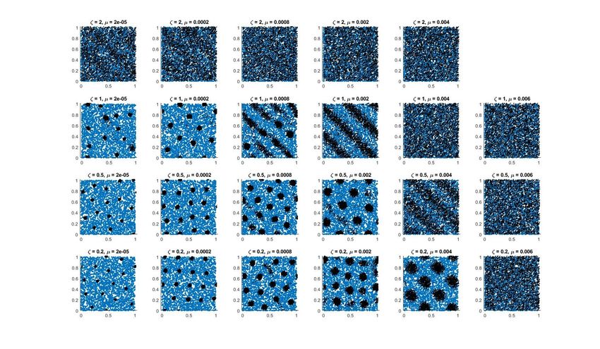
Contents
1 Introduction                                                                                                                                                           3

2 Modeling                                                                                                                                                               5
  2.1 Discrete dynamics . . . . . . .               . . . . . .             .   .   .   .   .   .   .   .   .   .   .   .   .   .   .   .   .   .   .   .   .   .   .    5
  2.2 Continuum dynamics . . . . . .                . . . . . .             .   .   .   .   .   .   .   .   .   .   .   .   .   .   .   .   .   .   .   .   .   .   .    6
      2.2.1 Main assumptions of the                 derivation              .   .   .   .   .   .   .   .   .   .   .   .   .   .   .   .   .   .   .   .   .   .   .    6
      2.2.2 The continuum model .                   . . . . . .             .   .   .   .   .   .   .   .   .   .   .   .   .   .   .   .   .   .   .   .   .   .   .    7

3 Patterns: phase diagrams                                                                                                                                               9
  3.1 Discrete dynamics . . .       .   .   .   .   .   .   .   .   .   .   .   .   .   .   .   .   .   .   .   .   .   .   .   .   .   .   .   .   .   .   .   .   .    9
      3.1.1 Simulation set up       .   .   .   .   .   .   .   .   .   .   .   .   .   .   .   .   .   .   .   .   .   .   .   .   .   .   .   .   .   .   .   .   .    9
      3.1.2 Phase diagram .         .   .   .   .   .   .   .   .   .   .   .   .   .   .   .   .   .   .   .   .   .   .   .   .   .   .   .   .   .   .   .   .   .    9
  3.2 Continuum dynamics . .        .   .   .   .   .   .   .   .   .   .   .   .   .   .   .   .   .   .   .   .   .   .   .   .   .   .   .   .   .   .   .   .   .   10
      3.2.1 Simulation set up       .   .   .   .   .   .   .   .   .   .   .   .   .   .   .   .   .   .   .   .   .   .   .   .   .   .   .   .   .   .   .   .   .   10
      3.2.2 Phase diagram .         .   .   .   .   .   .   .   .   .   .   .   .   .   .   .   .   .   .   .   .   .   .   .   .   .   .   .   .   .   .   .   .   .   12

4 Linear stability of uniform states                                                                                                                                    13
  4.1 Analysis of the continuum model . . . . . . . . . . . . . . . . . . . . . . . . . . . .                                                                           13
  4.2 Numerical validation of the linear stability analysis . . . . . . . . . . . . . . . . . .                                                                         17
      4.2.1 Predictions from the theoretical analysis and qualitative agreement with the
             macroscopic simulations . . . . . . . . . . . . . . . . . . . . . . . . . . . . .                                                                          17
      4.2.2 Quantitative agreement between the macroscopic simulations and the stabil-
             ity analysis . . . . . . . . . . . . . . . . . . . . . . . . . . . . . . . . . . . .                                                                       21

5 Quantitative assessment of the continuum model                                                                                                                        21
  5.1 Methodology to compare discrete and continuum simulations                                                         .   .   .   .   .   .   .   .   .   .   .   .   21
      5.1.1 Discretization of the particle density . . . . . . . . . .                                                  .   .   .   .   .   .   .   .   .   .   .   .   23
      5.1.2 Comparing discretized and discrete dynamics . . . . .                                                       .   .   .   .   .   .   .   .   .   .   .   .   24
  5.2 Results . . . . . . . . . . . . . . . . . . . . . . . . . . . . . . .                                             .   .   .   .   .   .   .   .   .   .   .   .   27
      5.2.1 Mild obstacle spring stiffness . . . . . . . . . . . . . .                                                  .   .   .   .   .   .   .   .   .   .   .   .   28
      5.2.2 Strong obstacle spring stiffness . . . . . . . . . . . . .                                                  .   .   .   .   .   .   .   .   .   .   .   .   30
      5.2.3 Summary of observations . . . . . . . . . . . . . . . .                                                     .   .   .   .   .   .   .   .   .   .   .   .   32

6 Discussion                                                                                                                                                            32

A Supplementary material: Videos of IBM simulations                                                                                                                     36

B Supplementary material: Numerical codes for the Individual-Based Model and
  Continuous Model simulations                                               37

C Numerical method for the continuum model                                                                                                                              37

                                                                    2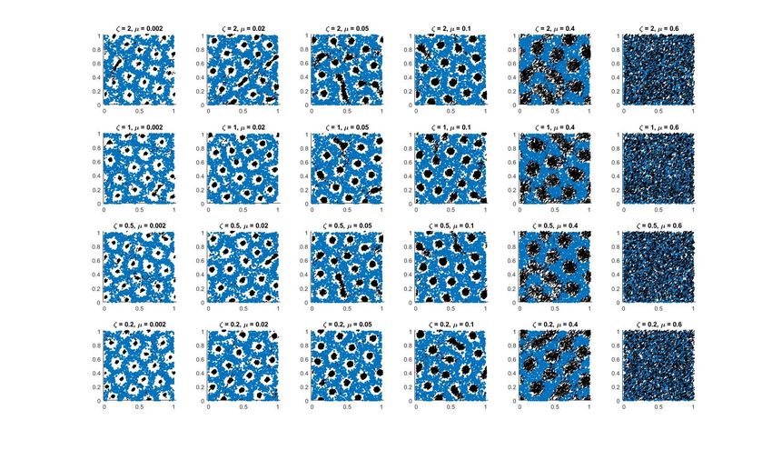
Figure 1: Overview of the paper. It includes a summary of the scales, the models and the objects
considered in this paper and introduced in [17] (first three grey lines). The blue boxes indicate
the derivation of the different models and derivation assumptions. The main contributions in the
paper appear in the last row corresponding to ‘patterns’ (at the discrete and continuum level and
their correspondence) and the linear stability analysis (bottom right yellow box).

1    Introduction
Understanding how patterns in collective motion arise from local interactions between individuals
is an exciting and challenging endeavour that has drawn the attention of the scientific community
[3, 4, 8, 5, 12, 21, 32, 36]. In many scenarios the environment plays a key role in the emergence
of collective motion and of the resulting patterns [9, 25, 27, 28, 34, 37]. Examples are evacuation
dynamics in the presence of obstacles [18, 21, 29], sperm dynamics in the seminal fluid [14, 37],
swirl of fish under the presence of predators [7], cells moving in a space filled with fibers [27] or
over a substrate [32],...
In particular, we are interested by feedback interactions between self-propelled agents and their
environment that they are able to modify. This happens, for example, (i) in the formation of
paths in grass-land by active walkers [22, 26],(ii) in the modification of the extra-cellular matrix
(fibers) by migratory cells [2], or (iii) in ant trail formation due to ant pheromone deposition [5].
In this paper, we will focus on the model introduced in [17] where collective motion happens in
an environment filled with movable obstacles that are tethered to a fixed point via a spring. The
authors in [17] showed that a variety of patterns are generated due to the feedback interactions
between the obstacles and the self-propelled agents. Indeed, the capacity of the agents to modify
their environment (i.e., to modify the position of the obstacles) is key for patterns to form.
    Figure 1 offers an overview of the ideas and messages of this paper. We will consider mostly

                                                 3
two scales (marked in yellow). The reason for this is that understanding the emergent properties of
collective dynamics requires to establish a link between the agent’s interactions and the continuum
dynamics that emerges at scales much larger than the size of the individual agents. As a conse-
quence, it is natural to consider two different scales to investigate collective motion: a microscopic
scale where the discrete dynamics of the agents can be described, and a macroscopic scale where
the average/continuum behaviour of the large ensemble can be observed.
    From a modelling perspective, it is natural to consider the microscopic scale, where individual-
based models can describe individual-agent behaviour and their interactions. In the left column
of Figure 1 we present key features of the individual-based model introduced in [17]. The model
assumes that agents move trying to avoid obstacles via a repulsion force. Agents interact with each
other following Vicsek-type dynamics [13, 20, 24, 38], i.e. they move at a constant speed trying to
align their orientation of motion with the one of their neighbours, up to some noise, while repelling
each other at short distances. The discrete system gives the time-evolution of the position of the
obstacles (Xi )i=1,...,N tethered at fixed anchor points (Yi )i=1,...,N via a spring and the position and
orientation of the self-propelled agents (Zk , αk )k=1,...,M , where Xi , Yi , Zk ∈ R2 and αk is a unit
vector (see Eq. (1) for a full mathematical description of the system and Figure 1 for a list of the
most relevant parameters). We will explore the variety of patterns that arise depending on the
values of the model parameters.
    However, the simulation of the discrete model becomes quickly computationally challenging
for systems composed of millions of individuals. Therefore, for large-particle systems, continuum
models are to be preferred since they provide information on the average behaviour and are compu-
tationally less costly (right column of Figure 1). Moreover, continuum models are the appropriate
framework for studying large scale patterns and carry out mathematical analyses like linear stabil-
ity analysis. The drawback is that, from a modelling perspective, they are harder to justify than
individual based models. For this reason, one would like to derive the continuum dynamics from
the discrete ones: this derivation validates the continuum models and provides understanding on
the emergence of large-scale patterns. At the same time, during this derivation process, due to
averaging and asymptotic analysis, some information on the discrete system can be lost.
    This rigorous derivation is precisely one of the purposes of kinetic theory. Kinetic theory has
been successfully applied to the study of models like the Vicsek model [13, 20, 24, 38] and the
Cucker-Smale model [1, 6, 10]. Tools from kinetic theory were applied in [17] to the discrete model
described above, see second and third rows in Figure 1.
    First, the authors derive the mean-field limit equation (large-particle limit N, M → ∞ for both
agents and obstacles). This equation corresponds to a Kolmogorov-Fokker-Plank equation for the
time-evolution of the distribution of the agents g = g(z, α, t) at position z ∈ R2 and orientation α;
and the time-evolution of the distribution of the obstacles f = f (x, y, t) at position x ∈ R2 with
anchor point at y ∈ R2 .
    Then, from the kinetic equations for these distributions, the authors in [17] obtained continuum
equations for the system under some asymptotic assumptions on the parameters (right blue boxes
in Figure 1). In particular, it is assumed a high stiffness of the obstacle springs, strong local agent-
agent repulsion and fast agent alignment. In this regime, it was shown in [17] that the obstacle
density ρf = ρf (x, t) becomes a non-local function of the agent density ρg = ρg (x, t) and that the
continuum model consists of a system of two non-linear non-local equations for ρg and the local
mean orientation of the agents Ω = Ω(x, t), see Eqs. (6).

   The main objective of this article is to investigate the influence of the tethered obstacles in
pattern formation using the discrete and continuum models first introduced in [17]. The main
contributions of this paper are listed below:
   • We focus our study primarily on the continuum equations (which were analysed only in
     dimension one in [17]). Here we introduce 2D simulations of the continuum equations and
     an extensive phase diagram (Sec. 3.2) that shows the appearance of patterns depending on
     the value of the parameters (green box in Fig. 1). We carry out a linear stability analysis
     in 2D around uniform states and validate this analysis by comparing its predictions with the

                                                   4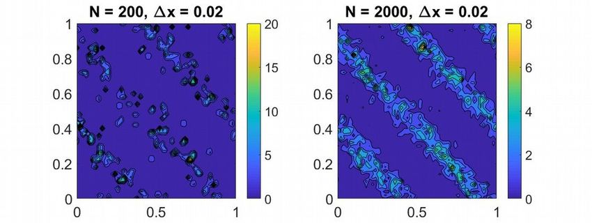
numerical simulations of the discrete and continuum models (right yellow box in Fig. 1).
    • We document in which parameter regime the continuum equations capture the discrete pat-
      terns (bottom grey box in Fig. 1). To this aim, we propose a method to compare discrete
      and continuum simulations. This novel method provides an indicator of the distance between
      different patterns.
    • Lastly, we also expand and greatly systematize the parameter exploration of the discrete
      model supported by a phase diagram. As a consequence, we detect two new patterns with
      respect to reference [17]: honeycombs structures and pinned agents states (left green box in
      Fig. 1).

Organisation of the paper. The paper is organized as follows: we first describe the models
(discrete and continuum), including the derivation assumptions of the continuum model. Then we
simulate both systems to construct two corresponding phase diagrams based on different values of
the parameters. Next, to better understand pattern formation as function of the model parameters,
we perform a linear stability analysis of the continuum equations around uniform states and identify
bifurcation parameters controlling the formation of patterns. Finally, an innovative method is
proposed to compare discrete and continuum simulations, which is used to determine in which
parameter regime the continuum equations are in good accordance with the discrete dynamics.
We conclude the paper with a discussion of the main results.

2     Modeling
2.1    Discrete dynamics
We consider as a starting point the model introduced in [17] for self-propelled particles undergoing
collective motion in an environment filled with obstacles. Obstacles are tethered to a given fixed
anchor point through a Hookean spring. They are characterised by their positions Xi (t) ∈ R2
over time t ≥ 0 and their anchor points Yi ∈ R2 for i = 1, 2, . . . , N , where N is the total number
of obstacles. The self-propelled particles are characterised by their positions Zk (t) ∈ R2 and
orientations αk (t) ∈ S1 (unit circle) at time t ≥ 0, k = 1, 2, . . . , M , where M is the total number
of agents. We assume that obstacles and agents interact through a given potential, as explained
next.
    The evolution for the obstacles (Xi (t), Yi )i=1,...,N and the agents (Zk (t), αk (t))k=1,...,M over
time is given by the following coupled system of stochastic differential equations:
                                               M
                         κ                 1 1 X                   p
               dXi = −     (Xi − Yi ) dt −       ∇φ (Xi − Zk ) dt + 2do dBti ,                     (1a)
                         η                 ηM
                                                   k=1
                                      N                         M
                                1 1 X                      1 1 X
              dZk =u0 αk dt −           ∇φ (Zk − Xi ) dt −          ∇ψ (Zk − Zl ) dt,              (1b)
                                ζ N i=1                    ζM
                                                               l6=k
                                      p
               dαk =Pα⊥
                      k
                          ◦ ν ᾱk dt + 2ds dB̃tk ,                                                 (1c)

where the mean direction ᾱk is defined via the mean flux Jk as follows
                                                                 M
                                          Jk                     X
                                 ᾱk =         ,   where Jk =          αj .                         (2)
                                         |Jk |                    j=1
                                                             |Zk −Zj |≤rA

Eq. (1a) gives the time-evolution for the obstacles’ positions Xi . The first term on the right-
hand side corresponds to the force generated by the Hookean spring anchored at position Yi with
stiffness constant κ > 0. The tether positions Yi are given and do not change over time. The terms

                                                         5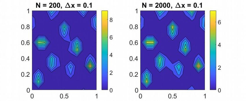
B i , i = 1, . . . , N are independent Brownian motions that introduce noise in the dynamics with
intensity d0 > 0. This term accounts for fluctuations in the dynamics. Finally, the second term on
the right-hand side of Eq. (1a) is precisely the interaction force that couples the dynamics of the
self-propelled agents with the ones of the obstacles. We assume that φ is an even and non-negative
interaction potential. Typically we will assume φ to be a repulsive potential to model volume
exclusion between obstacles and self-propelled particles.
     Now, Eq. (1b) gives the time-evolution for the position of the self-propelled agents Zk . The
first term on the right-hand-side of (1b) expresses that agent k moves in the orientation αk at a
fixed speed u0 > 0. The second term is the force due to the interaction potential coupling the
self-propelled agents and the obstacles, as we have seen before. Finally, the last term is a repulsive
force between agents given by a potential ψ which is assumed to be non-negative and even. This
force is added to the model to prevent agents clustering at a single point in space and represents
volume exclusion interactions between the agents [12].
     The last equation (1c) gives the time-evolution for the orientation of the agents and corresponds
to the terms appearing in the Vicsek model [15] which is a widely used model in collective motion.
The right hand side of Eq. (1c) is the sum of two competing forces: a force that tries to align the
orientation of the self-propelled agents with the mean orientation of their neighbours and a noise
term that opposes this alignment. The noise is given by (B̃ k )k=1,...,M which are M independent
Brownian motions (also assumed to be independent from B i , i = 1, . . . , N ) and the intensity
of this noise is given by the parameter ds > 0. The operator Pα⊥          k
                                                                             represents the orthonormal
projection onto αk⊥ (where αk⊥ is a vector orthogonal to αk ) and the symbol 0 ◦0 indicates that the
stochastic differential equation has to be understood in the Stratonovich sense [23]. In particular,
the projection ensures that, for all times where the dynamics are defined, αk (t) remains on the
sphere, i.e., |αk | = 1. The alignment force is given by Pα⊥   k
                                                                 ν ᾱk where ν > 0 is a positive constant
and ᾱk is the average orientation of the neighbouring agents that are at distance rA > 0 from
agent k, as computed in Eq. (2). Indeed, this term corresponds to an alignment force since it can
be rewritten as
                                        Pα⊥
                                          k
                                            ν ᾱk = ν∇αk (αk · ᾱk ),
where ∇αk denotes the gradient on the sphere. Therefore, this term is a gradient flow that relaxes
αk towards the average orientation ᾱk at speed ν > 0.

    Finally, notice that the discrete model (1) consists of first order equations: the model can be
derived from second order equations in the overdamped (or inertialess) regime. This is the reason
why the parameters η > 0 and ζ > 0 appear in the system: η corresponds to the obstacle friction
and ζ to the agent friction. In an inertialess regime first-order equations give a good approximation
of the dynamics and this regime appears in many biological applications, in particular involving
micro-agents (like sperm cells) in highly viscous environments.
    As we will see in later sections, the feedback interactions between agents and between agents
and obstacles give rise to a variety of patterns depending on the value of the parameters.

2.2     Continuum dynamics
When the number of agents and obstacles becomes large, it is useful to derive equations that
determine the average behaviour of the discrete system (1). These ‘averaged’ equations correspond
to continuum equations, which were derived in [17] for the discrete system (1). In this section we
summarise the results from this reference.

2.2.1   Main assumptions of the derivation
The derivation of the continuum equations in [17] is done under the following set of assumptions:

(a) Large-particle-system assumption. The number of obstacles and agents are assumed to
tend to infinity, i.e., N → ∞, M → ∞.

                                                   6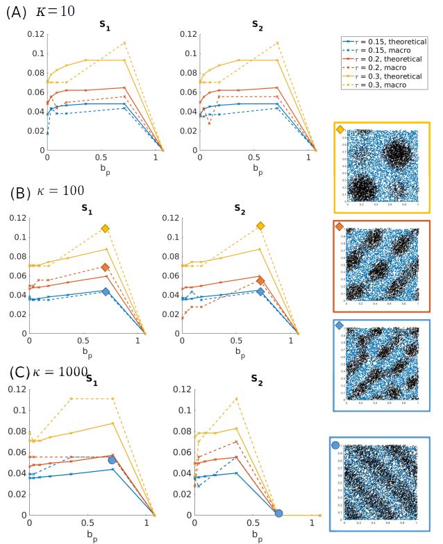
Under this assumption, the authors derived formally equations for the evolution of obstacles and
agent density (kinetic equations). Then, some of the parameters of the kinetic equation are scaled
by a small factor ε  1 and the continuum equations are obtained in the limit ε → 0. We explain
next the scaling assumptions considered.

(b) Scaling assumptions on the parameters. Three types of scaling assumptions          √ are made:
(i) the radius of alignment of the agents is supposed to be small and scaled as rA = O( ε); (ii) the
agent-agent repulsion distance is supposed to be small and scales as rR = O(ε), but it is ensured
that the potential stays of order 1 by setting
                                        Z
                                            ψ(x)dx = µ < ∞;                                      (3)

(iii) the agents alignment rate ν and orientational noise intensity ds in (1c) are supposed to be very
large and scale as: ds , ν = O( 1ε ) with dνs = O(1): this corresponds to fast agent-agent alignment
and diffusion [15].

(c) Uniform anchor density and stiff regime assumptions. It is assumed that the anchor
density for the obstacles is constant (uniformly distributed) and that the obstacles’ springs are
very stiff (the parameter κ is very large). To this aim, we consider the ratio
                                                   η
                                              γ=     1                                           (4)
                                                   κ
to be small. We suppose also a low obstacle noise regime, by considering the smallness of
                                             δ = do γ  1.                                        (5)

    The set of assumptions (a) is sufficient to derive continuum equations. The large-particle-limit
or mean-field limit gives rise to kinetic equations for the obstacle density f = f (t, x, y) and the
agent density g = g(t, z, α). The set of assumptions (b) and (c) are sufficient to obtain closed
equations for the obstacle density ρf = ρf (t, x), the agent density ρg = ρg (x,
                                                                               √ t) and the mean-
agent orientation Ω = Ω(x, t). In particular, the scaling assumptions rA = O( ε) and rR = O(ε)
imply that alignment and agent-agent repulsion forces become localized in space as ε → 0. The
set of assumptions (c) is used to Taylor expand the function f with respect to γ and δ.

   In summary, the continuum equations approximate a system with a very large number of
agents and obstacles in the regime where the parameters of the system reach a given range of
values, as described above, i.e., in the regime ε → 0 (by an asymptotic analysis) and γ ≈ 0, δ ≈ 0
(by a Taylor expansion approximation). These approximations will be taken into account when
comparing discrete and continuum simulations, since they determine the range of validity of the
continuum dynamics.

2.2.2   The continuum model
The authors in [17] obtain the following equations for the dynamics of the density of agents
ρg (x, t) ∈ R and their mean orientation Ω(x, t) ∈ S1 at a point x ∈ R2 at time t ≥ 0:
                        ∂t ρg + ∇ · (U ρg ) = 0,                                                  (6)
                        ρg ∂t Ω + ρg (V · ∇) Ω + d3 PΩ⊥ ∇ρg = γs PΩ⊥ ∆(ρg Ω),
where
                                               1      µ
                                     U = d1 Ω − ∇ρ̄f − ∇ρg ,
                                               ζ      ζ
                                               1      µ
                                     V = d2 Ω − ∇ρ̄f − ∇ρg ,
                                               ζ      ζ

                                                   7
where ρf (x, t) is the obstacle density given by:

                    1       1            η               η 3
        ρf /ρA = 1 + ∆ρ̄g + 2 N (ρ̄g ) − 2 ∂t ∆ρ̄g + O        ,                        N (ρ̄g ) := detH(ρ̄g ),     (7)
                    κ      κ            κ                κ

where ρA is the distribution of the anchor points in space (assumed to be constant and here taken
to be equal to 1 in the simulations and computations); H denotes the Hessian, ‘det’ denotes the
determinant, and we have defined
                                            ρ̄ := ρ ∗ φ,                                      (8)
the convolution between ρ and φ, where φ is the repulsion kernel between agents and obstacles,
Eq. (12). In the numerical simulations we will drop the higher order terms in η/κ for ρf . The
model parameters are the friction constants ζ, η, the obstacle-spring constant κ, and the agent-
agent repulsion intensity µ given by Eq. (3).
   The friction coefficient γs reads

                                              r2

                                                          ds
                                          γs = A             + c2 .                                                (9)
                                               8          ν

   The constants d1 , d2 and d3 are defined by

                                                   di = u0 ci ,                                                   (10)

where u0 is the agent speed, and c1 , c2 and c3 are explicit constants that depend only on the
fraction ds /ν:
                                         Z   2π
                                  c1 =            cos θ m(θ) dθ,                                                 (11a)
                                         R0π 2
                                          0R
                                            sin θ cos θ m(θ)h(θ) dθ
                                  c2 =       π                      ,                                            (11b)
                                            0
                                               sin2 θ m(θ)h(θ) dθ
                                  c3 = ds /ν,                                                                    (11c)

where                                                            Z   2π
                         1             ν
                   m(θ) = exp             cos θ ,           Z :=            exp(ν cos θ/ds ) dθ.
                         Z             ds                          0

and where the function h does not have a explicit form but it is the solution to a differential
equation. Specifically, h(θ) = g(θ)/ sin(θ) where g is the unique solution (for the exact functional
space in which this unique solution is defined, the reader is referred to [12, Lemma 2.3])

                                        ν        dg d2 g
                                           sin θ    + 2 = sin θ.
                                        ds       dθ  dθ

    For an explanation on the meaning of these equations the reader is referred to [17]. We just point
here that the system (6) for (ρg , Ωg ) corresponds to the so-called Self-Organised Hydrodynamics
with Repulsion (SOHR) [12] in the case where ∇x ρ̄f = 0 (i.e. when there is no influence from the
obstacles). The SOHR is the continuum version of the Vicsek model with agent-agent repulsion
[12].
Remark 1 (Approximation for ρf and blow-up). The density ρf may take negative values: in
that case the continuum simulations will bestopped. Notice also that solutions may ‘blow-up’ in the
sense that particle densities may concentrate at points in space.

                                                        8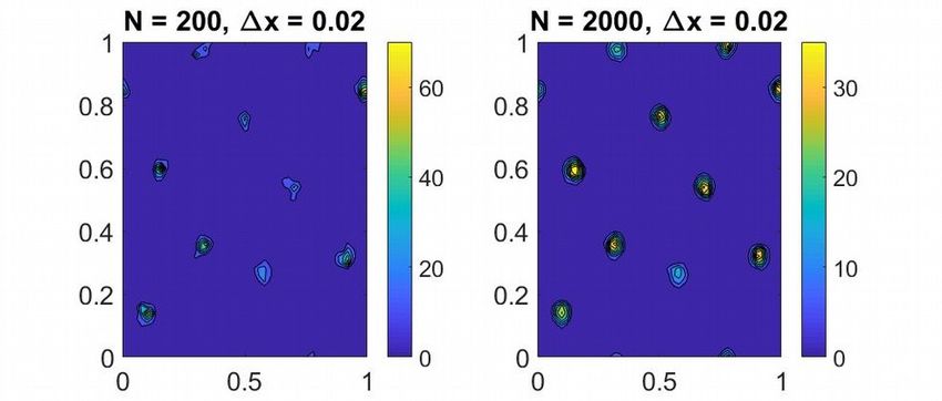
3 Patterns: phase diagrams
3.1 Discrete dynamics
3.1.1 Simulation set up
We here show some simulations of the discrete model (1) to give an overview of the different types
of patterns that emerge depending on the values of the parameters. Simulations are performed
with N = M = 3000 agents and obstacles initially distributed uniformly in the periodic domain
U = [0, 1]×[0, 1]. We also suppose that anchor points Yk for the obstacles are uniformly distributed
in U , and fix the initial agent direction to π/4.
We consider the following expressions for the agent-agent and agent-obstacle repulsion poten-
tials: 2 2
6µ |x| 3Cφ |x|
ψ(x) = 2 1 − , φ(x) = 1− , (12)
πrR rR + 2πτ τ +
where
if x2 ∈ R+ ,
x
x2+ =
0 if x < 0.
Therefore, both potentials are compactly supported and act in a radius rR > 0 for agent-agent
repulsion and a radius τ > 0 for agent-obstacle repulsion. Notice that the constants have been
chosen such that Z Z
µ = ψ(x)dx and Cφ = |∇φ|(x)dx.
We fix a set of parameters as described in Table 1, and focus our study on the interplay between
three parameters: the obstacle spring stiffness κ, the agent friction ζ and the agent-agent repulsion
intensity µ.
3.1.2 Phase diagram
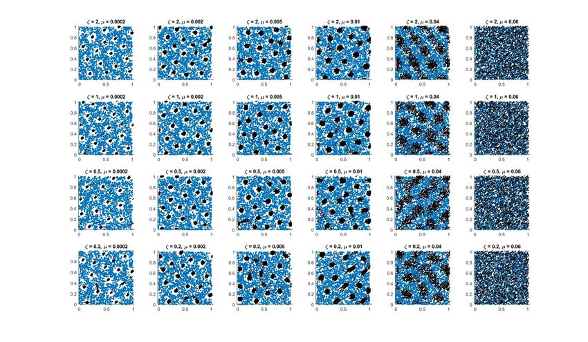
Fig. 2 shows the output of the simulations at time t = 10: at this time agents and obstacles
patterns seem to have reached a steady state. In this figure, agents’ positions and their orientations
are represented with black arrows and obstacle’s positions with blue dots. The output of the
simulations are grouped into three panels: panel (A) corresponds to weak obstacle spring stiffness
κ = 10, and panels (B) and (C) correspond to mild κ = 100 and strong κ = 1000 obstacle
spring stiffness, respectively. Inside each panel, we arrange the simulations in a table: right-to-left
columns correspond to increasing values of the agent-agent repulsion force µ, bottom-to-top rows
correspond to increasing values of the friction coefficient ζ. Notice that the value for the agent-
agent repulsion force µ is not taken the same in all panels. Indeed, the values for µ selected are the
ones that make different patterns appear in the simulations. We will justify further the particular
choice of the parameters after the linear stability analysis of the continuum equations. Notice that
the values for ζ are also different in panel (C). We refer the reader to the caption of Fig. 2 for the
exact choices for the parameter values of µ and ζ. Finally, we point out that the figures marked
with a red cross are the ones for which the videos can be found in the supplementary material (see
Appendix A for more details).
From Fig. 2 we observe that a rich variety of agents’ patterns emerges when varying the spring
stiffness κ, the intensity of the agent-agent repulsion µ, and the friction coefficient ζ.
We classify these patterns into 4 main types and we outline the parameter regions corresponding
to each with frames of different colors in Fig. 2:
• Trails of agents (framed in red): agents organize into trails inside the obstacle pool. This
behavior is mainly observed for weak and mild obstacle spring stiffness (κ = 10, panel (A)
and κ = 100, panel (B) of Fig. 2, respectively)
9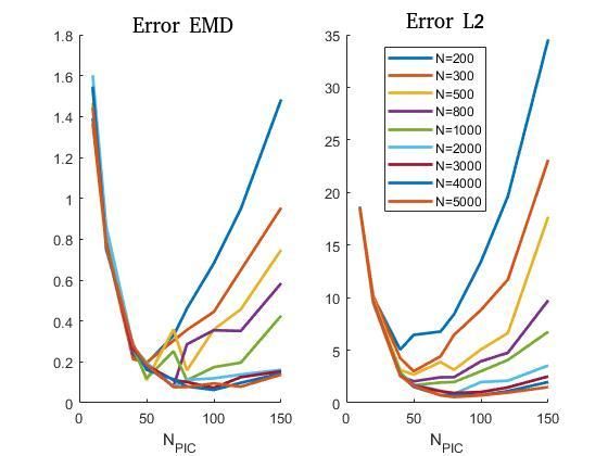
• Honeycomb organization of the agents (framed in orange): For small obstacle spring stiffness
     κ = 10 (panel (A) of Fig. 2) and mild agent-agent repulsion µ > 0.1 (middle columns),
     we observe that the agents organize into fixed honeycomb structures, framing the obstacles
     which concentrate into aggregates of different sizes and shapes (not necessarily round). We
     point out that this pattern was not detected in the previous publication [17].
   • Travelling bands of agents (framed in yellow): only observed for large values of the obstacle
     spring stiffness κ = 103 and large agent friction with the environment ζ = 5, here the agents
     organize into bands perpendicular to their direction of motion. The width of the bands
     increases with the agent-agent repulsion intensity µ (from left to right plots of the first row
     of panel (C)).
   • Clusters of agents (framed in green): agents organize into clusters more or less round depend-
     ing on the regime of parameters. Cluster formation appears in all regimes of obstacle spring
     stiffness κ = 10, 102 , 103 (all three panels), and the size of the clusters changes depending
     on the obstacle spring stiffness κ and on the agent-agent repulsion intensity µ but seems
     independent of the agent friction ζ. Particularly, we observe that the cluster sizes increase
     with µ, until a point is reached in which µ is so large that agent-agent repulsion counteracts
     all the other aggregation forces (right columns of Fig. 2). Moreover, the parameter µ acts as
     a phase transition parameter between different types of patterns. During the transition from
     clustered to near-homogeneous agent distributions with increasing repulsion intensity µ, we
     observe a passage to other pattern types such as trails (for weak κ = 10 or mild κ = 100
     obstacle stiffness), or honeycomb organizations (for weak obstacle stiffness). Finally, we note
     that for large obstacle spring stiffness κ and small agent friction ζ (bottom row of panel (C),
     simulations marked with a green star) we observe the formation of ’pinned’ clusters where the
     agents are grouped into very small clusters that do not move (see Supplementary material
     and Appendix A for access to the videos)
Each of these agent patterns is surrounded by obstacles that are kept at a given distance from
the agents. This distance depends on the stiffness of the obstacles’ springs κ and the agent-agent
repulsion intensity µ. On one hand, if obstacles are loose enough (i.e., κ is small), the repulsion
force between the agents and the obstacles may be large enough to keep them both at approximately
the obstacle-agent repulsion distance τ (defined in the potential φ, Eq. (12)). On the other hand,
agent-agent repulsion opposes this effect, by giving the agent population force to go against the
pressure exerted by the obstacle pool. We indeed observe that increasing the agent-agent repulsion
force µ (left-to-right columns of Fig. 2) decreases the typical distance between the agent structures
and the obstacles.

3.2     Continuum dynamics
In this section we show numerical simulations of the continuum equations (6) using the numerical
scheme detailed in Appendix C.

3.2.1   Simulation set up
We perform simulations of the continuum model on the periodic domain U = [0, 1] × [0, 1] dis-
cretized with space step ∆x ≈ 6.7 10−3 (150 discretization points in each direction). The initial
homogeneous agent directionR Ω0 is set to π4 , and initial agent density ρg is a small perturbation of
a uniform distribution with Ω ρg = 1. In order to compare the numerical results with the discrete
model, we use the same parameters as for the discrete simulations presented in Section 3.1 (see
Table 2).
    Notice that the agent-agent alignment distance at the continuum level is chosen to be rA = 0.15
whereas for the discrete simulations it was 0.1. This   √ choice corresponds    to having rescaled rA
                                                  0                    0
approximately by a scaling factor ε = 0.5, i.e., rA  = εrA , where rA    = 0.1 is the parameter used
in the discrete simulation (see the scaling assumption (b) in Sec. 2.2.1). Note that only the ratio

                                                 10
(A) Weak obstacle spring stiffness
Increasing friction coefficient
Increasing swimmer-swimmer repulsion
(B) Mild obstacle spring stiffness
Increasing friction coefficient
Increasing swimmer-swimmer repulsion
(C) Strong obstacle spring stiffness
Increasing friction coefficient
Increasing swimmer-swimmer repulsion
Figure 2: Simulations of the discrete model for the parameters indicated in table 1. Agents
are represented as black arrows giving their direction of motion, obstacles are represented
as blue circles. Panel (A): for weak obstacle stiffness κ = 10, panel (B): for mild ob-
stacle stiffness κ = 100, panel (C): for large obstacle stiffness κ = 1000. In each
panel, the vertical axis represents different values of the friction coefficient ζ (from bot-
tom to top: ζ = 0.2, 0.5, 1, 2 for panels (A) and (B) and ζ = 0.2, 1, 2, 5 for panel (C);
and the horizontal axis represents different values11 of the agent-agent repulsion µ: panel (A):
µ ∈ {0.002, 0.02, 0.05, 0.1, 0.4, 0.6} , panel (B): µ ∈ {0.0002, 0.002, 0.005, 0.01, 0.04, 0.06}, panel
(C): µ ∈ {2.10−5 , 2.10−4 , 6.10−4 , 2.10−3 , 4.10−3 , 6.10−3 }.Parameters Value Description
N 3000 number of obstacles
M 3000 number of agents
u0 1 agent speed
rR 0.075 agent-agent repulsion distance
rA 0.1 agent-agent alignment distance
ν 2 agent-agent alignment intensity
τ 0.15 agent-obstacle repulsion distance
Cφ 5 agent-obstacle repulsion intensity
ds 0.02 noise in the agents’ orientation
η 1 obstacle friction
d0 0 obstacle positional noise
µ various agent-agent repulsion intensity
ζ various friction constant of the agents
κ various spring constant coefficient
Table 1: Parameters used for the discrete simulations of Fig. 2. The various values considered for
µ, ζ, κ are specified in the caption of Fig. 2.
Parameters Value Description
h ≈ 6.7 · 10−3 step-size spatial discretization
v0 1 agent speed
rA 0.15 agent-agent alignment distance
ds
ν 0.01 parameter coming from alignment forces
τ 0.15 agent-obstacle repulsion distance
Cφ 5 agent-obstacle repulsion intensity
η 1 obstacle friction
γs 28 · 10−4 viscosity coefficient
µ various agent-agent repulsion intensity
ζ various agent friction constant
γ various γ = η/κ
Table 2: Parameters used for the simulations of the continuum equations (6) shown in Fig. 3. The
constants d1 , d2 , d3 only depend on ν/ds and are obtained by computing the expressions (10) and
(11).
ds /ν is relevant for the continuous model, independently of their individual values. We therefore
just ensure that this ratio is kept the same as for the discrete simulations and use ds /ν = 0.01.
3.2.2 Phase diagram
We present the output of the continuum simulations. To facilitate the comparison with the discrete
system, we adopt the same representation as the one presented in Fig. 2. In particular, the
continuum densities are discretized as follows: at a simulation time t we distribute randomly
N = 3000 agent points in the domain according to the distribution ρg (·, t), and similarly for the
obstacle points using ρf (·, t). In Fig. 3 we show the simulation results at the final time of the
simulation, corresponding either to the time before blow-up or appearance of negative density for
the obstacles (see Rem. 1) or to t = 10, as for the discrete simulations. As in Fig. 2, the simulations
are separated in three panels: panel (A) is obtained for weak obstacle stiffness κ = 10, and panels
(B) and (C) are for κ = 100 and κ = 1000 respectively. In each panel, we organize the simulations
in tables for which bottom-to-top rows correspond to increasing values of the friction coefficient
ζ, while left-to-right columns correspond to increasing values of the agent-agent repulsion force
12intensity µ. See the legend of Fig. 3 for more details on the parameter values considered for ζ and
µ.
In Fig. 3 we observe different patterns for the agents, each framed using the same color code
as for the discrete simulations: cluster formation (framed in green, present in all three panels),
travelling bands (framed in yellow, panel (C), trails (framed in red, panel (B)), near-honeycomb
structures (framed in orange, panel (A)), uniform distributions (unframed) and in-between states.
Here again, increasing the obstacle spring stiffness κ (from top to bottom panels) decreases the
distance between agents and obstacles (i.e., the white area around the agents is reduced with
increasing κ). We also observe that increasing the agent-agent repulsion intensity µ increases the
size of the agent clusters and this parameter again serves as a transition parameter between clusters
and uniform distribution of the agents, passing through honeycomb structures (first row of panel
(A)), trails (third row of panel (B)) or travelling bands (first three rows of panel (C)). The effect
of the friction parameter ζ becomes more relevant for large values of κ. For example, in panel (C)
the parameter ζ serves as a transition parameter between clusters, trails and uniform states.
Comparing phase diagrams. We compare the two phase diagrams from the discrete simula-
tions in Fig. 2 and the continuum simulations in Fig. 3. Note, though, that there is not an exact
correspondence of the values for the parameter ζ used in panel (C) for the two cases.
It is noteworthy that the patterns observed with the continuum simulations are similar to the
patterns of the discrete simulations (Fig. 2) for strong and mild obstacle spring stiffness (compare
panels (B) and (C) of Figs. 3 and 2), while the two models lead to different types of behavior
in the weak obstacle stiffness regime (panel (A)). These are expected results since the continuum
model has been obtained in a strong obstacle spring stiffness regime (1/κ ≈ 0). As a result,
the continuum model seems to be unable to produce the rich variety of patterns offered by the
discrete model when considering loose obstacles. Also, we do not observe the pinned state with
the continuum model, which appeared with the discrete dynamics when considering large obstacle
spring stiffness κ and small agent friction ζ. Even though pinned-states are observed for large
values of κ, they correspond to states where agents collapse into a very small cluster and then
the numerical simulations of the continuum equations blow-up due to a high concentration of the
agent density ρg (see Rem. 1).
4 Linear stability of uniform states
4.1 Analysis of the continuum model
Continuum equations are amenable to linear stability analysis around constant solutions or uniform
states. This is useful because the presence of instabilities signals the formation of patterns. In this
section we obtain an explicit condition for the stability of uniform states.
Before stating the main result, we introduce the following notation: denote by φ̂ the Fourier
transform of φ defined as, for k ∈ R2 :
Z
φ̂k := φ̂|k| = φ̂(k) = e−ik·x φ(x)dx ∈ R.
R2
Notice that φ is assumed rotationally invariant, therefore φ̂ is real and rotationally invariant (so
we abused notation and wrote φ̂|k| instead of φ̂k ).
Theorem 1 (Linear instability). Consider fixed constant values ρ0 > 0 and Ω0 ∈ S1 . Then, the
linearized system of (6) around (ρ0 , Ω0 ) is unstable if and only if
there exists z > 0 such that z 2 (φ̂z )2 > µκ. (13)
The proof of the theorem is given later. First, we derive sufficient conditions for the system to
be stable:
13(A) Weak obstacle spring stiffness
Increasing friction coefficient
Increasing swimmer-swimmer repulsion
(B) Mild obstacle spring stiffness
Increasing friction coefficient
Increasing swimmer-swimmer repulsion
(C) Strong obstacle spring stiffness
Increasing friction coefficient
Increasing swimmer-swimmer repulsion
Figure 3: Simulations of the continuum model (6) for the parameters indicated in table 2. Agents
(randomly distributed from the distribution ρg (x, t)) are represented as black arrows of orientation
π/4, obstacles (randomly distributed from the distribution ρf (x, t)) are represented as blue circles.
panel (A): for weak obstacle stiffness κ = 10, panel (B): for mild obstacle stiffness κ = 100, panel
(C): for large obstacle stiffness κ = 1000. In each panel, the vertical axis represents different values
of the friction coefficient ζ (from bottom to top: ζ = 0.2, 0.5, 1, 2 and the horizontal axis represents
different values of the agent-agent repulsion µ:14panel (A): µ ∈ {0.002, 0.02, 0.05, 0.1, 0.4, 0.6},
panel (B): left column: µ ∈ {0.0002, 0.002, 0.005, 0.01, 0.04, 0.06}, panel (C):
µ ∈ {2.10−5 , 2.10−4 , 6.10−4 , 2.10−3 , 4.10−3 , 6.10−3 }.Corollary 1 (Conditions for stability). Suppose that φ is absolutely continuous, rotationally in-
variant, and φ, φ0 ∈ L1 . Then, it holds that
c0 := max z 2 (φ̂z )2 < ∞ (14)
z∈R+
and if µκ > c0 , then the continuum equations (6) are linearly stable.
Moreover, if φ is given by (12), define c00 = c0 /Cφ2 . It holds that the constant c00 is independent
on the obstacle-agent repulsion radius τ and the intensity Cφ and the system is stable whenever
µκ
> c00 .
Cφ2
Proof. Since by assumption φ is absolutely continuous and φ, φ0 ∈ L1 , we have that |φ̂0 (k)| = |k||φ̂(k)|.
Moreover, since φ0 ∈ L1 , then φ̂0 is bounded. Therefore, |k|2 |φ̂(k)|2 is bounded and c0 is finite. In
this case, for µκ > c0 the instability condition (13) does not hold, so the system is stable.
In the particular case where φ takes the shape given in (12), one can check that the following
self-similarity condition holds
|k|φ̂k = τ|k|φ̂(1) (τ|k|),
where φ(1) corresponds to φ when taking τ = 1. Therefore, it holds that
Cφ2 c0 = max |k|2 (φ̂k )2 = max(τ|k|)2 (φ̂(1) (τ|k|))2 = max |y|2 (φ̂(1) (|y|))2 ,
k k y
and so c0 is independent of τ. The rest of the corollary follows: the value of c00 is also clearly
independent of Cφ as it is just a multiplicative factor of φ.
Remark 2 (Limiting case of pillar obstacles). In the case where the obstacles are fixed pillars,
i.e., the case where κ → ∞, then the uniform distribution of agents and pillars is always a stable
solution. The effect of this limiting case is that the equations for the agents on (ρg , Ω) become
decoupled from the obstacles’ density ρf = ρA , which is just constant (take the formal limit κ → ∞
on the continuum equations (6)). Therefore, there is an abrupt behavioural change between static
obstacles and obstacles that can move a bit (anchored at a fixed point via a very stiff spring). This
shows that, in this particular set up, the fact that the agents are able to modify their environment
is crucial for interesting patterns to emerge.
The role of the parameters. From the instability condition (13), we observe that the main
drivers of the formation of instabilities are: the shape of the agent-obstacle repulsion potential
φ, the obstacle-spring stiffness κ, and the agent-agent repulsion intensity µ. High agent-agent
repulsion - high values of µ - has a stabilising effect while high agent-obstacle repulsion - high
values of Cφ - has a destabilising effect, and vice-versa. Also, high values of the spring constant κ
have a stabilising effect and small values have the opposite effect.
From Cor. 1, in the case when φ is given in (12) the ratio given by
µκ
bp := (15)
Cφ2 c00
is the single value that acts as a bifurcation parameter. However, the obstacle-agent repulsion
radius τ plays a role in determining the size of the patterns (see Fig. 3). Also, from the instability
condition (13) and corollary 1, for typical shapes of the potential φ, we expect to have stability
for small and large values of the wave vector k but instabilities can appear at intermediate values
whenever c0 > µκ (where c0 is given in (14)).
The rest of this section is devoted to the proof of Th. 1.
15Proof of Th. 1. We start by linearising the continuum equations (6) around (ρ0 , Ω0 ) by expanding
the solution using a small perturbation parameter β
ρg = ρ0 + βρ1 + O(β 2 ), Ω = Ω0 + βΩ1 + O(β 2 ), |Ω| = 1. (16)
Dropping the higher order terms, we obtain the linearised system (where the over-script bar nota-
tion is defined in Eq. (8)):
∂t ρ1 + d1 Ω0 · ∇ρ1 + d1 ρ0 ∇ · Ω1 = µ̄ρ0 ∆ρ1 + ρ0 λ̄ ∆2 ρ̄¯1 − γ∆2 ∂t ρ̄¯1 ,
(17a)
ρ0 ∂t Ω1 + ρ0 d2 (Ω0 · ∇) Ω1 + d3 PΩ⊥
0
∇ρ1 = γs ρ0 PΩ⊥
0
∆Ω1 , (17b)
Ω0 · Ω1 = 0, (17c)
where ∆2 is the bi-Laplacian, i.e., ∆2 ρ = ∆(∆ρ) and PΩ⊥ 0
is the orthogonal projection on Ω⊥0.
Note also that µ̄ = µ/ζ, γ = η/κ and λ̄ = ρA /(κζ) (we assume ρA = 1).
We now define the functions F, G : R+ → R by:
ρ0 1 2
F (z) := z 2 z (φ̂z )2 − µ , (18)
ζ κ
η
G(z) := 1 + ρ0 2 z 4 (φ̂z )2 > 0,
κ ζ
and given k ∈ R2 , we denote by k0 , k1 the quantities
k0 = (k · Ω0 ), k1 = (k · Ω⊥
0 ), (19)
where Ω⊥ 0 is the image of Ω0 by the rotation of angle π/2. Th. 1 is then a direct consequence of
the following proposition.
Proposition 1. System (17) allows for non-trivial plane wave solutions, i.e. solutions of the form
ρ1 (x, t) = ρ̃eik·x+αt , Ω1 (x, t) = Ω̃eik·x+αt , (20)
2 2
where k ∈ R is the wave vector, α ∈ C, ρ̃ ∈ C and Ω̃ ∈ C , and (ρ̃, Ω̃) 6= (0, 0) if and only if α
and k fulfil the following dispersion relations:
Case A: k k Ω0
Option 1: ρ̃ 6= 0, Ω̃ = 0,
d1 k0 F (|k0 |)
α = α1 (k) := −i + . (21)
G(|k0 |) G(|k0 |)
Option 2: ρ̃ = 0, Ω̃ 6= 0.
α = α2 (k) := −id2 k0 − |k|2 γs . (22)
Case B: k ∦ Ω0 . Then, α is a root of the following polynomial of degree 2:
α2 G + α G|k|2 γs − F + ik0 (Gd2 + d1 )
(23)
d1 (ρ0 d3 k12 d2 k02 ) 2 2
+ − − |k| γs F + i d1 k0 |k| γs − d2 k0 F = 0.
The real parts of α are negative if and only if the following holds:
G(k)|k|2 γs − F (k) > 0, (24)
and
2
H(k) := G(k)|k|2 γs − F (k) d1 d3 k12
(25)
h 2 i
−γs F (k)|k|2 (d1 − d2 G(k))2 k02 + G(k)|k|2 γs − F (k)
> 0.
16Proof of Prop. 1. Substituting the plane wave ansatz into the equation yields
ρ̃α + iρ̃d1 (Ω0 · k) + iρ0 d1 Ω̃ · k = −|k|2 µ̄ρ0 ρ̃ + |k|4 λ̄ρ0 ρ̃(φ̂k )2 (1 − γα) , (26a)
ρ0 αΩ̃ + iρ0 d2 Ω̃ (Ω0 · k) + iρ̃d3 PΩ⊥
0
k = −|k|2 ρ0 γs Ω̃, (26b)
Ω0 · Ω̃ = 0. (26c)
or (if Ω̃ = ωΩ⊥
0)
(G(|k|)α − F (|k|) + id1 k0 )ρ̃ + iρ0 d1 k1 ω = 0,
id3 k1 ρ̃ + ρ0 (α + id2 k0 + |k|2 γs )ω = 0.
This is a homogeneous linear system in (ρ̃, ω) which has a non-trivial solution if and only if the
determinant of the system is 0, i.e.:
(G(|k|)α − F (|k|) + id1 k0 ) α + id2 k0 + |k|2 γs + d1 d3 k12 = 0.
(27)
If k1 = 0, there are two roots corresponding to either bracket being zero. This leads to (21) or
(22). If k1 6= 0, we can recast (27) in (23).
To determine the sign of the real part of α, we use the Routh-Hurwitz criterion for polynomials
with complex coefficients [19, 30]. In our case the Routh-Hurwitz criterion states that the Re(α) < 0
for all solutions α if and only if expressions (24) and (25) hold.
With Prop. 1 we conclude the proof of Th. 1 as follows. Suppose (13) holds and let z0 > 0
be such that z02 φ̂2z0 > µκ. Let k = z0 Ω0 . Then k0 = z0 and k1 = 0. So F (|k|) = F (z0 ) > 0 and
α = α1 (k) is such that Re (α) > 0. Hence, the linearized system is unstable.
Suppose now (13) does not hold, i.e., z 2 φ̂2z < µκ, for all z ∈ R+ . Then, F (|k|) < 0, for all
k ∈ R2 . It results that Re(α1 (|k|)) < 0, Re(α2 (|k|)) < 0. Furthermore (24) and (25) are obviously
satisfied for all k ∈ R2 . Hence the system is stable.
4.2 Numerical validation of the linear stability analysis
In this section we compare the pattern predictions given by the linear stability analysis with the
results obtained from numerical simulations. This way we check that the linear stability analysis
truly captures pattern formation, i.e., that nonlinear effects are of second order and most of the
patterns characteristics are captured by linear effects.
4.2.1 Predictions from the theoretical analysis and qualitative agreement with the
macroscopic simulations
We start by giving insights on the size and shape of the expected patterns based on the theoretical
predictions offered by the stability analysis. To this aim, we consider perturbations introduced
in the stability analysis (see Prop. 1), around the homogeneous density ρ0 = 1 and in constant
direction Ω0 ∈ S1 . As we are particularly interested in characterizing the patterns corresponding
to clusters or bands, we will focus on the theoretical values for wave vectors parallel to Ω0 and
parallel to Ω⊥
0 :
kkth = argmax Re(α̃(k)), k⊥ th
= argmax Re(α(k)),
kkΩ0 kkΩ⊥
0
where α̃(k) corresponds to case A (Eq. (21)), α(k) corresponds to case B (larger root of Eq.
(23), computed numerically) and the symbol ‘Re’ indicates the real part. With these wave vectors
maximizing the real part of α, we define the quantities:
2π 2π
S1th = , S2th = .
|kkth | th |
|k⊥
17Figure 4: Prediction of the linear stability analysis. Left: values of the maximal growth rate
of the plane wave perturbations in the direction of Ω0 (continuous lines) and in the orthogonal
direction Ω⊥0 (dashed lines) as functions of the bifurcation parameter bp , for different values of the
agent friction ζ: ζ = 0.1 (blue curves), ζ = 0.5 (red curves), ζ = 1 (yellow curves). Right: same
representation for the size of the perturbations in the two directions S1th and S2th .
These quantities give the size of the expected patterns in each direction. We will also compute the
maximal growth rates of the perturbations in these two directions:
k ⊥
αmax = max Re(α̃(k)), αmax = argmax Re(α(k)).
kkΩ0 kkΩ⊥
0
Equipped with these quantifiers, we now study the influence of the model parameters on the
expected pattern shapes and sizes. As predicted by the stability analysis, patterns can be expected
if the bifurcation parameter bp (Eq. (15)) is below 1. We fix Cφ = 5 and use φ as in Eq. (12)
giving c0 ≈ 5.6 independent on τ as shown in the proof of corollary 1 (definition of c0 in Eq. 14).
We vary bp by changing the values of the agent-agent repulsion intensity µ and aim to study the
influence of the friction constant ζ, the obstacle spring stiffness κ and the agent-obstacle repulsion
distance τ. For each subsection, we compare qualitatively these predictions based on the linear
stability analysis with simulations of the macroscopic model presented in Fig. 3
Influence of the friction constant ζ. First we fix κ = 1000 and τ = 0.15, and show in Fig.
k ⊥
4 the values of αmax and αmax (left panel) and of S1th and S2th (right panel), as functions of the
bifurcation parameter bp and for different values of the agent friction constant ζ: ζ = 0.1 (blue
curves), ζ = 0.5 (red curves), ζ = 1 (yellow curves). One can first observe in Fig. 4 (left panel)
that we indeed recover the critical value 1 of the bifurcation parameter, below which perturbations
grow (Re(α) > 0) and after which they are damped, independently on the value of ζ. This shows
that bp is indeed a relevant bifurcation parameter. Moreover, one can observe that perturbations
grow faster for smaller values of the friction constant ζ (compare the blue and red curves in the
left panel). From the right panel of Fig. 4, we note first that the size of the clusters increases
when increasing the bifurcation parameter (here, by increasing the agent-agent repulsion µ). These
are expected results as stronger agent repulsion leads to higher pressure in the agent population,
leading to larger clusters. Secondly, we observe that the size of the patterns is independent on
the friction constant ζ, but the parameter zone in which patterns are of travelling band type (i.e
S1th > 0 and S2th = 0) is larger for larger values of ζ -compare the yellow and blue dashed curves
in the right panel-. Thus, high friction substrates seem to favor the formation of travelling bands
compared to low friction environments, provided the bifurcation parameter is large enough (large
obstacle spring stiffness and/or large agent-agent repulsion compared to agent-obstacle repulsion).
Qualitative comparison with the macroscopic simulations. The influence of the agent
friction ζ for τ = 0.15 and κ = 1000 can be observed in the macroscopic simulations presented in
18Figure 5: Left: values of the maximal growth rate of the plane wave perturbations in the direction
of Ω0 (continuous lines) and in the orthogonal direction Ω⊥ 0 (dashed lines) as functions of the
bifurcation parameter bp , for different values of the obstacle spring stiffness κ: κ = 10 (blue
curves), κ = 100 (red curves), κ = 1000 (yellow curves). Right: same representation for the size of
the perturbations in the two directions S1th and S2th .
Fig. 3 panel (C), comparing the rows together (from bottom to top for increasing values of ζ).
We first note that in the simulations of the three panels of Fig. 3, the values considered for the
product µκ were always the same, i.e.,
µκ ∈ {0.02, 0.2, 0.5, 1, 4, 6},
and the value of Cφ = 5 was kept constant, corresponding to the following values for the bifurcation
parameter:
bp ∈ {0.0036, 0.0357, 0.0893, 0.1785, 0.7142, 1.0713}.
We then observe that in each panel of Fig. 3, patterns are indeed observed in the first 5 columns
of the tables while the last column displays a homogeneous distribution of agents. This validates
the fact that patterns are observed only when the bifurcation parameter bp is below 1.
Moreover, focusing on the last panel (for which κ = 1000), we recover most of the observations
predicted by the stability analysis: (a) the pattern size increases when increasing the bifurcation
parameter (increasing µ: compare simulations from left to right in Fig. 3 panel (C)), (b) the zone
of parameters showing travelling bands increases when increasing the agent friction ζ (compare
bottom to top rows of panel (C)). Therefore, we obtain a very good qualitative agreement between
the simulations of the macro model and the tendencies predicted by the stability analysis as function
of ζ.
Influence of the obstacle spring stiffness κ. Here we adopt the same representation as in
the previous paragraph, but fixing the agent friction constant ζ = 0.5 and playing on the obstacle
k
spring stiffness κ (we keep the agent-obstacle distance τ = 0.15). Fig. 5 shows the values of αmax
⊥ th th
and αmax (left panel) and of S1 and S2 (right panel), as functions of the bifurcation parameter
bp and for κ = 10 (blue curves), κ = 100 (red curves) and κ = 1000 (yellow curves). From Fig.
5 (right), we can observe a similar evolution of the pattern size playing on the obstacle spring
stiffness as when changing the friction constant ζ: increasing the obstacle spring stiffness κ slightly
increases the zone of parameters favoring the formation of bands of agents (compare yellow and
red dashed curves in the right panel). One can particularly note (blue curve of Fig. 5 (right)) that
environments composed of loose obstacles (κ = 10) will only promote agent clusters the size of
which is independent of the value of the bifurcation parameter. Finally we note from Fig. 5 (left)
that the growth rate of perturbations does not evolve monotonically with the spring stiffness κ:
faster perturbations are observed for κ = 100 compared to κ = 10 or κ = 1000 (compare red with
blue and yellow curves in the left panel).
19Figure 6: Left: values of the maximal growth rate of the plane wave perturbations in the direction
of Ω0 (continuous lines) and in the orthogonal direction Ω⊥ 0 (dashed lines) as functions of the
bifurcation parameter bp , for different values of the agent-obstacle distance τ: τ = 0.15 (blue
curves), τ = 0.2 (red curves), τ = 0.3 (yellow curves). Right: same representation for the size of
the perturbations in the two directions S1th and S2th .
Qualitative comparison with the macroscopic simulations. The influence of the obstacle
spring stiffness κ for τ = 0.15 and ζ = 0.5 can be observed in the macroscopic simulations presented
in Fig. 3, comparing the second rows (starting from the bottom) in each panel (panel (A) for κ = 10,
panel (B) for κ = 100, panel (C) for κ = 1000).
Again, we obtain a very good agreement with the theoretical predictions: (a) the pattern sizes
increase when increasing the bifurcation parameter (by increasing µ: compare simulations from
left to right in each panel), (b) the increase in pattern size as function of µ seems less important for
κ = 10 (panel (A)) than for larger obstacle spring stiffness (panels (B) and (C)), and (c) travelling
bands are only observed for κ = 1000 (panel (C)).
Influence of the agent-obstacle repulsion distance τ
Finally we aim to document the role of the agent-obstacle repulsion distance τ. We adopt the
same methodology as in the two previous paragraphs: we fix ζ = 0.5 and κ = 1000 and show in
k ⊥
Fig. 6 the values of αmax and αmax (left panel) and of S1th and S2th (right panel), as functions
of the bifurcation parameter bp and for τ = 0.15 (blue curves), τ = 0.2 (red curves) and τ = 0.3
(yellow curves). We first observe that increasing the value of τ slows down the growth of the
perturbation modes (compare blue red and yellow curves of Fig. 6 (left)). Moreover, as predicted
by the stability analysis, the critical value of µ for which patterns appear does not depend on τ:
patterns are once again only observed as long as the bifurcation parameter bp does not exceed the
value 1. Secondly, Fig. 6 (right) shows that the agent-obstacle distance τ has a strong impact on
the size of the clusters: larger τ leads to larger agent clusters (compare for instance yellow and
blue curves in Fig. 6 (right)), and agent-obstacle repulsion distance does not impact the shape of
the patterns (clusters or bands types).
As the simulations of Fig. 3 have been generated only for τ = 0.15, we are not able at this
point to compare qualitatively the predictions of the stability analysis with the simulations of the
macroscopic model as functions of this parameter. We will however assess the influence of τ via a
quantitative comparison between the model and the theory in the next section.
Altogether, these results show that agent-agent repulsion favors the spreading of the agents
while agent-obstacle repulsion tends to aggregate the agents (and consequently clusters obstacles
together). Travelling bands of agents seem to be favored in low friction environments composed of
stiff obstacles, and the size of agent clusters seem to be controlled primarily by the agent-obstacle
distance and the bifurcation parameter (ratio between the agent-agent repulsion intensity and the
agent-obstacle repulsion intensity).
20You can also read