Graphics processing unit implementation of the F -statistic for continuous gravitational wave searches
←
→
Page content transcription
If your browser does not render page correctly, please read the page content below
Graphics processing unit implementation of the
                                        F-statistic for continuous gravitational wave
                                        searches
arXiv:2201.00451v1 [gr-qc] 3 Jan 2022

                                                     Liam Dunn1,2 , Patrick Clearwater3,1,2 , Andrew Melatos1,2 , and
                                                     Karl Wette4,2
                                                     1
                                                       School of Physics, University of Melbourne, Parkville VIC 3010, Australia
                                                     2
                                                       ARC Centre of Excellence for Gravitational Wave Discovery (OzGrav), Hawthorn
                                                     VIC 3122, Australia
                                                     3
                                                       Gravitational Wave Data Centre, Swinburne University of Technology, Hawthorn
                                                     VIC 3122, Australia
                                                     4
                                                       Centre for Gravitational Astrophysics, Australian National University, Canberra
                                                     ACT 2601, Australia
                                                     E-mail: liamd@student.unimelb.edu.au

                                                     Abstract. The F -statistic is a detection statistic used widely in searches for
                                                     continuous gravitational waves with terrestrial, long-baseline interferometers. A
                                                     new implementation of the F -statistic is presented which accelerates the existing
                                                     “resampling” algorithm using graphics processing units (GPUs).              The new
                                                     implementation runs between 10 and 100 times faster than the existing implementation
                                                     on central processing units without sacrificing numerical accuracy. The utility of the
                                                     GPU implementation is demonstrated on a pilot narrowband search for four newly
                                                     discovered millisecond pulsars in the globular cluster Omega Centauri using data from
                                                     the second Laser Interferometer Gravitational-Wave Observatory observing run. The
                                                     computational cost is 17.2 GPU-hours using the new implementation, compared to
                                                     1092 core-hours with the existing implementation.

                                        Submitted to: Class. Quantum Grav.
GPU F -statistic 2
1. Introduction
Gravitational waves emitted by isolated and accreting neutron stars [1] are a key
target for terrestrial, long-baseline interferometers, such as the Laser Interferometer
Gravitational-wave Observatory (LIGO) [2], Virgo [3], and the Kamioka Gravitational
Wave Detector (KAGRA) [4]. Individual neutron stars are continuous wave sources;
they emit persistent harmonic signals as they rotate. Continuous wave searches
are typically limited in sensitivity and parameter range by available computational
resources. This is particularly true when the astrophysical parameters (e.g. the
neutron star spin frequency and/or binary orbital elements) are poorly constrained by
electromagnetic observations. Continuous wave sources are relatively weak compared to
the compact binary coalescences which have been detected already. These coalescences
have typical peak gravitational-wave strains of order 10−22 [5, 6], while the current
most stringent 95% confidence level upper limits on the gravitational-wave strain from
continuous wave sources are of order 10−25 for all-sky searches with wide parameter
spaces [7, 8], and of order 10−26 for targeted searches for emission from known pulsars
[9, 10]. Sensitivity to these weak continuous wave sources is enhanced by integration
over long time spans (hundreds of days), posing a further computational challenge.
A promising approach for dealing with computationally-heavy problems is to
reformulate them to take advantage of graphics processing units (GPUs). GPUs can
execute thousands of tasks in parallel, in contrast to the dozens of tasks which can be
performed by a modern, multi-core central processing unit (CPU). They are particularly
well-suited to “embarrassingly parallel” problems, which can be broken down into simple
sub-steps, where each sub-step performs the same instructions on different data, and
few sub-steps depend on the results of other sub-steps. Frameworks such as CUDA [11]
and OpenCL [12], which enable general-purpose computing on GPUs, have unleashed
the power of GPUs on a range of applications in industry and science. In the field
of gravitational wave astronomy in particular, GPUs have been brought to bear on
problems such as the low-latency detection of compact binary coalescences [13, 14],
Bayesian inference applied to compact binary coalescences [15,16], searches for long-lived
transient signals [17], and a search for continuous gravitational waves from Scorpius X-1
[18]. Recently, a new GPU-based implementation of the FrequencyHough algorithm [19]
for all-sky continuous wave searches has been reported [20], achieving a speed-up of 1–2
orders of magnitude over the existing CPU-based implementation. The application of
deep learning techniques to the analysis of both compact binary coalescences [21, 22]
and continuous gravitational waves [23] has also benefited greatly from the computing
power provided by GPUs.
One of the principal tools employed in continuous-wave searches is the F -statistic,
introduced by [24]. This is a maximum-likelihood technique requiring numerical
maximisation over certain parameters which control the evolution of the phase of the
signal at the detector. It has been applied to searches for electromagnetically discovered
targets at known sky locations [25] and all-sky surveys for unknown targets [26]. TheGPU F -statistic 3
LIGO Algorithms Library Suite (LALSuite) [27] currently contains two implementations
of the F -statistic [28]: the demodulation algorithm (Demod) [29], which is older and
typically runs slower; and the resampling algorithm (Resamp) [30], which typically runs
faster. Both implementations operate on CPUs.
In this paper we present a new implementation of the resampling algorithm, which
offloads most of the computation to GPUs, achieving substantial speed-up over the
CPU implementation. The paper is structured as follows. In section 2 we review the
mathematical definition of the F -statistic, so that it is clear what data it accepts as
input and what arithmetic and logical operations it entails. In section 3 we outline the
algorithmic steps involved in calculating the F -statistic and explain how to implement
these steps within the CUDA framework for GPU programming. In section 4 we evaluate
the runtime (section 4.1) and accuracy (section 4.2) of the GPU implementation, and
compare against the CPU implementations available in LALSuite. In section 5 we
describe a pilot search using the GPU implementation to target four newly discovered
millisecond pulsars in the globular cluster Omega Centauri [31], using data from the
second LIGO-Virgo observing run (O2). Neutron stars in Omega Centauri have not
been the subject of any targeted or directed searches for continuous gravitational waves
previously. Nevertheless we emphasise that the search described here is only a proof of
principle demonstrating the utility of the GPU implementation of the F -statistic, not
a full-scale astrophysical search. Finally in section 6 we discuss future prospects for
additional optimisation and the implications for future F -statistic searches with LIGO
data.
2. F -statistic
The F -statistic is a detection statistic which is constructed from the likelihood ratio
Pr[x | HS (A, λ)]
L(x; A, λ) ≡ . (1)
Pr[x | HN ]
Conditional probabilities are denoted Pr[· | ·], and following the notation of [32], the
observed data are denoted by x, A is the set of “amplitude parameters” determining
the amplitude of the signal at the detector, and λ is the set of “phase parameters”
which determine the evolution of the phase of the signal at the detector. The two
hypotheses are HN , the hypothesis that the data consist solely of Gaussian noise with
known power spectral density, and HS (A, λ), the hypothesis that the data consist of
Gaussian noise with known power spectral density, plus a continuous wave signal with
parameters A, λ. The likelihood ratio L(x; A, λ) can be analytically maximised over A,
leaving the maximum-likelihood function
LML(x; λ) = max L(x; A, λ) = eF (x,λ) . (2)
A
The final equality in (2) serves as the definition of F (x, λ) (hereafter written as F for
brevity).GPU F -statistic 4
In practice F is calculated via two Fourier transforms of the data, weighted by the
two antenna beam pattern functions of the detector. The phase of a continuous wave
signal from a rotating neutron star can be written as [24]
h i
(k)
Φ(t) = 2πf0 [t + tm (t; α, δ)] + Φs t; f0 , α, δ , (3)
where tm gives the time offset due to the motion of the detector, and Φs gives the phase
due to the rotational evolution of the source. Here α and δ are the right ascension and
(k)
declination of the source, f0 is the gravitational-wave frequency, f0 is the k-th time
derivative of the gravitational-wave frequency, and Φs is expressed as a Taylor series in
(k)
time, whose coefficients are given by f0 (k ≥ 1). Following [24] throughout, we define
the two integrals
Z Tobs /2
Fa (f0 ) = dt x(t)a(t) exp[−iΦs (t)] exp{−i2πf0 [t + tm (t)]}, (4)
−Tobs /2
Z Tobs /2
Fb (f0 ) = dt x(t)b(t) exp[−iΦs (t)] exp{−i2πf0 [t + tm (t)]}, (5)
−Tobs /2
where Tobs is the total observing time, x(t) is the data time series in the detector
frame, and a(t) and b(t) encode the beam-pattern functions, also in the detector frame.
Explicit formulas for a(t) and b(t) are given by equations (12) and (13) of [24] in terms
of α, δ, and the detector’s orientation. Introducing a new barycentred time coordinate,
tb (t) = t + tm (t), and making the approximations tb (Tobs /2) ≈ Tobs /2 and dt/dtb ≈ 1,
we rewrite (4) and (5) as
Z Tobs /2
Fa (f0 ) = dtb x[t(tb )]a[t(tb )] exp{−iΦs [t(tb )]} exp(−i2πf0 tb ), (6)
−Tobs /2
Z Tobs /2
Fb (f0 ) = dtb x[t(tb )]b[t(tb )] exp{−iΦs [t(tb )]} exp(−i2πf0 tb ). (7)
−Tobs /2
The detection statistic F is defined as
4 B|Fa |2 + A|Fb |2 − 2Cℜ(Fa Fb∗ )
F= , (8)
Sh (f0 )Tobs D
where A, B, C, and D = AB − C 2 are integrals of products of a(t) and b(t) over
−Tobs /2 ≤ t ≤ Tobs /2 (i.e. constants depending on α and δ), and Sh (f0 ) is the one-sided
power spectral density of the detector noise at the frequency f0 .
Equations (6) and (7) are standard Fourier transforms of the data x[t(tb )] multiplied
by the slowly varying functions a[t(tb )] and b[t(tb )], with |ȧ| ≪ f0 |a| and |ḃ| ≪ f0 |b|.
Hence they can be computed efficiently using standard CPU and GPU libraries, e.g.
FFTW and cuFFT [33].
3. GPU Implementation
We develop a CUDA implementation of the F -statistic based on the Resamp algorithm,
suggested by [24] and elaborated and implemented by [30], whose notation we follow.GPU F -statistic 5
A mature CPU-based implementation of Resamp already exists in LALSuite. The CUDA
implementation is a fairly direct “translation” of the CPU code. It hooks in smoothly
to the rest of the LALSuite infrastructure. In particular, it is easily usable with the
ComputeFStatistic v2 program, which wraps the various F -statistic routines available
in LALPulsar (the portion of LALSuite containing routines for continuous GW data
(k)
analysis), and provides logic for parameter searches over f0 , f0 , α, and δ for example.
In practice, the starting point for analysis is not the raw time series x(t) but rather
a sequence of short Fourier transforms (SFTs). These are discrete Fourier transforms of
the detector output over time segments which are short enough (typically TSFT ∼ 1800 s)
that amplitude and phase modulations due to the Earth’s motion and the source’s
frequency evolution are small.
The Resamp method consists of the following steps for a single detector; the
generalization to multiple detectors is straightforward.
(i) Combine the SFTs into a single Fourier transform.
(ii) Complex heterodyne at a frequency fh , downsample, and low-pass filter the data in
the frequency domain. Perform an inverse Fast Fourier Transform (FFT) to obtain
the time series xh (tk ), where k goes from 1 to the total number of samples, and tk
is regularly spaced in the detector frame.
(iii) Correct xh (tk ) to account for the fact that the heterodyning operation occurs in
the detector frame rather than the Solar System barycentre frame. The result,
z(tk ) = xh (tk )ei2πfh tm , is heterodyned in the Solar System barycentre frame but is
sampled irregularly in that frame.
(iv) Choose tkb , a series of regularly spaced epochs in the Solar System barycentre
frame. Calculate T k (tkb ), the epochs in the detector frame corresponding to regular
sampling in the Solar System barycentre frame.
(v) Calculate z T k (tkb ) by interpolating z(tk ).
(vi) Calculate Fa (f − fh ) and Fb (f − fh ), by computing the FFTs of
a T k (tkb ) z T k (tkb ) exp −iΦs T k (tkb ) and b T k (tkb ) z T k (tkb ) exp −iΦs T k (tkb ) .
(vii) Calculate F (f − fh ) from (8).
Note that a single pass of the procedure (i)–(vii) can be used to compute F over a
user-defined frequency band of width ∆f , centred on fh .
The process of converting a sequence of SFTs into the time series xh (tk ) is complex
(see Section III B of [30] for details) and does not present a significant computational
bottleneck, so we do not reimplement it. It is instead performed using the existing
CPU-bound code in LALSuite. Steps (iii), (iv), (v), and (vii) can be expressed neatly
as a simple operation or short sequence of operations executed independently for a
large number of data points, where these data points may be elements of the detector
data time series (either in the detector frame or the solar system barycentre frame), or
frequency bins in the F results. It is straightforward to write one or two CUDA kernels per
step, which carry out the computations in parallel. GPUs are extremely well-suited toGPU F -statistic 6
performing the FFTs in step (vi). An optimised FFT library for CUDA exists in cuFFT‡,
which we use here.
Steps (iii) through (vii) must be repeated for every search template [i.e. every
(k)
combination of α, δ, and f0 with k ≥ 1], so accelerating them with GPUs yields
computational savings which scale with the number of templates. In contrast, computing
xh (tk ) using GPUs would deliver a speed-up which is constant with the number of
templates. For now we are content to amortise the cost of calculating xh (tk ) over the
typically large number of templates, so that the proportion of computation performed
on the CPU decreases as the number of templates increases. The CPU time taken to
perform steps (i) and (ii) is typically on the order of seconds to a few minutes depending
on the nature of the data to be loaded, while the GPU time spent performing steps
(iii) to (vii) may be on the order of hours to days, when the number of templates is
large. We note also that the transfer of data from CPU memory to GPU memory
occurs only between steps (ii) and (iii) and is not repeated for every template, so this
cost (which might otherwise be substantial) is also amortised. The fact that all of the
template-dependent computation occurs on the GPU means that searches over large
numbers of templates can be carried out without introducing any inefficiencies due to
communication between the CPU and GPU. Thus searches over sky position α, δ and
(k)
spin-down parameters f0 incur no extra performance penalty beyond the run time
increasing in proportion to the number of templates. We are able to use all of the
existing infrastructure in LALSuite which manages these parameter space searches.
To give some idea of the similarities and differences between the CPU- and GPU-
based implementations, figure 1 shows a side-by-side comparison of code snippets from
the existing CPU code and the new CUDA code that perform step (vii) of the above
procedure.
4. Performance
To evaluate the performance of the CUDA implementation, we use the OzSTAR
computing cluster§, with compute nodes equipped with Intel Gold 6140 CPUs running
at 2.30 GHz (∼1011 floating point operations (FLOPs) per second per core), and Nvidia
P100 GPUs (∼1013 FLOPs per second). The benchmarking data were generated using
the Makefakedata v4 program in LALSuite.
We measure the performance of both the CPU and GPU implementations as a
function of two key parameters: the total coherent observing time Tobs , and the width
of the frequency band ∆f . These two parameters control the number of frequency bins
in the computation, which is the main factor determining the performance of the two
implementations. Varying other aspects of the computation, such as the number of
terms in the Taylor series for the signal phase model, has no discernible effect on the
performance of either implementation. We vary only one parameter at a time, keeping
‡ https://developer.nvidia.com/cufft
§ https://supercomputing.swin.edu.au/ozstar/GPU F -statistic 7
2 hb 2 b b |2 − 2C
b Re (Fa Fb∗ )
i
2F = B|Fa | + A|F
b
D
CPU CUDA
float *twoF = /************* CPU-side code *************/
֒→ malloc(sizeof(float)*numFreqBins); float *twoF_gpu;
for (size_t k = 0; k < numFreqBins; k++) cudaMalloc((void **)&twoF_gpu,
{ ֒→ sizeof(float)*numFreqBins);
twoF[k] = ComputeTwoF(ws->Fa_k[k], CUDAComputeTwoF>(twoF_gpu, ws->Fa_k,
֒→ ws->Fb_k, Ad, Bd, Cd, Ed, Dd_inv,
/**********************************/ ֒→ numFreqBins);
cudaMemcpy(Fstats->twoF, twoF_gpu,
static inline float ComputeTwoF(float complex ֒→ sizeof(float)*numFreqBins,
֒→ Fa, float complex Fb, float A, float B, ֒→ cudaMemcpyDeviceToHost);
֒→ float C, float E, float Dinv) cudaFree(twoF_gpu);
{
float Fa_re = creal(Fa); /************* GPU-side code *************/
float Fa_im = cimag(Fa); __global__ void CUDAComputeTwoF(float *twoF,
float Fb_re = creal(Fb); ֒→ cuComplex *Fa_k, cuComplex *Fb_k, float A,
float Fb_im = cimag(Fb); ֒→ float B, float C, float E, float Dinv,
float twoF = 2.0 * Dinv * (B * (Fa_re * ֒→ size_t numFreqBins)
֒→ Fa_re + Fa_im * Fa_im) + A * (Fb_re * {
֒→ Fb_re + Fb_im * Fb_im) - 2.0 * C * int k = threadIdx.x + blockDim.x *
֒→ (Fa_re * Fb_re + Fa_im * Fb_im) - 2.0 * ֒→ blockIdx.x;
֒→ E * (-Fa_re * Fb_im + Fa_im * Fb_re)); if (k >= numFreqBins) {
return twoF; return;
} }
cuComplex Fa = Fa_k[k];
cuComplex Fb = Fb_k[k];
float Fa_re = cuCrealf(Fa);
float Fa_im = cuCimagf(Fa);
float Fb_re = cuCrealf(Fb);
float Fb_im = cuCimagf(Fb);
float twoF_k = 2.0 * Dinv * (B * (Fa_re *
֒→ Fa_re + Fa_im * Fa_im) + A * (Fb_re *
֒→ Fb_re + Fb_im * Fb_im) - 2.0 * C *
֒→ (Fa_re * Fb_re + Fa_im * Fb_im) - 2.0 *
֒→ E * (-Fa_re * Fb_im + Fa_im * Fb_re));
twoF[k] = twoF_k;
}
Figure 1. Side-by-side comparison of CPU code (left) and CUDA code (right) used to
calculate 2F according to equation (134) from [28] (top), which is a rewriting of (8).
The quantities A, b B,
b C,
b Db −1 are normalised versions of the A, B, C, and D−1 that
appear in (8). Their definitions can be found in equation (133) of [28]. The variable
names in the code snippets are mostly self-explanatory, e.g. Fa re is the real part
of Fa (f0 ) defined in equation 4, and Dinv is Db −1 . The parameter E is zero in the
limit where the arm length of the detector is much smaller than the gravitational-wave
wavelength, which is always the case in the application considered here. Note that the
function ComputeTwoF in the CPU code takes the name compute fstat from fa fb in
the LIGO Algorithm Library.GPU F -statistic 8
∆f fixed at 0.606 Hz as Tobs is varied, and keeping Tobs fixed at 10 d as ∆f is varied.
These choices are illustrative and are typical of certain published, F -statistic-based
searches for accreting neutron stars, e.g. [18, 34–36]. For each parameter we search over
100 sky locations (α, δ) and average the timing results. All other parameters used in the
synthetic data generation and F -statistic computation are held fixed. The sky location
does not noticeably affect the speed of the computation, and provides a convenient way
to average the timing results over many executions of the algorithm without repeatedly
incurring the start-up costs associated with steps (i) and (ii) described in the previous
section.
We caution that the range of possible ∆f and Tobs combinations is limited by the
amount of memory available on the GPU. The scaling of required memory with both ∆f
and Tobs is approximately linear (with deviations due to padding to ensure that the FFTs
are carried out on data with lengths which are powers of two). As an indicative example,
the memory required for ∆f = 0.606 Hz, Tobs = 10 d is approximately 100 MB, a modest
amount compared to the several GB which are available on typical GPUs. However,
larger frequency bands and longer coherence times may present issues: increasing
both ∆f and Tobs by a factor of 10 requires approximately 10 GB of GPU memory,
approaching the limits of the Nvidia P100 GPUs used in testing which have 12 GB of
memory.
4.1. Runtime
We quote the performance results in terms of the timing coefficient τFeff introduced
by [37], defined as the time taken to calculate F for a single frequency bin in the
single-detector case, starting from the downsampled, complex heterodyned, and filtered
time series. We measure τFeff for the new CUDA implementation and the existing CPU-
bound implementation. The timing results are presented in figure 2. The leftmost and
middle panels give the absolute timing coefficients for the two implementations, while
the rightmost panels show the speed-up factor τFeff (CPU)/τFeff (GPU)
Figure 2 indicates that between one and two orders of magnitude of acceleration
is typical, with an overall trend towards higher τFeff (CPU)/τFeff (GPU) as the amount of
data grows.
The step jumps and subsequent declines in both the CPU and GPU timing results
occur because the data are padded, such that the dimension of the data vector is a power
of two, which greatly improves FFT performance. The jumps occur, when the number
of samples increases to the point, where the next power of two must be used, and there
is the greatest mismatch between the original number of samples and the number of
samples in the padded data.
Note that these timing results are averaged by searching over 100 sky locations for
each choice of Tobs or ∆f . Seaching over spin-down parameters instead (e.g. 100 values
(1)
of f0 ) leads to a ∼60% reduction in the computation time for the CPU implementation,
but only a ∼20% reduction in the computation time for the GPU implementation. InGPU F -statistic 9
×10−8 ×10−7
100
5.0 90
τFeff (CPU)/τFeff (GPU) (s)
80
1.0 4.5
τFeff (GPU) (s)
τFeff (CPU) (s)
70
4.0
60
3.5 50
0.5 3.0 40
1 10 100 1 10 100 1 10 100
Tobs (d) Tobs (d) Tobs (d)
×10−8 ×10⁻⁷
100
2.0
5.0 80
τFeff (CPU)/τFeff (GPU) (s)
1.5 60
4.5
τFeff (GPU) (s)
τFeff (CPU) (s)
1.0 4.0 40
3.5
0.5 20
3.0
0.1 1.0 2.0 0.1 0.5 1.0 2.0 0.1 0.5 1.0 2.0
∆f (Hz) ∆f (Hz) ∆f (Hz)
Figure 2. Comparative per-frequency bin runtime (τFeff in s) of the CPU (middle
column) and GPU implementations (left column) of Resamp. The right column displays
the speed-up factor τFeff (CPU)/τFeff (GPU). Top row : timing results as Tobs is varied,
with ∆f = 0.606 Hz. Bottom row : timing results as ∆f is varied, with Tobs = 10 d.
both cases the reduction in computation time is due to re-use of the results of the sky
position-dependent barycentering. This barycentering consumes a larger fraction of the
total computation time in the CPU case than in the GPU case. As a result, the overall
speed-up of the GPU implementation over the CPU implementation is reduced by a
factor of ∼2 when searching only over spin-down parameters, holding (α, δ) fixed.
We caution here that the values of τFeff refer only to the time taken to calculate
2F . The computational cost of any processing of the calculated 2F values (for example,
sorting to obtain the top 1% of candidates) is not included. In particular, τFeff (GPU)
does not include the time taken to transfer the calculated 2F values from GPU memory
back into CPU memory or to subsequently process those values using CPU-bound code.
Fortunately, the total amount of data to be transferred is not too great: the Nvidia P100
GPUs used in testing achieve a memory bandwidth of approximately 4.8 GB s−1 , and we
have to transfer 4 bytes (one single-precision floating point number) per frequency bin,
which costs an additional 8 × 10⁻¹⁰ s per frequency bin. Compared to τFeff ∼ 5 × 10⁻⁹ s,GPU F -statistic 10
Figure 3. Fractional error between the F -statistic computed with the GPU and CPU
implementations of Resamp for a single noise realisation and as a function of search
frequency f (in Hz). Injected signal parameters: h0 = 6 × 10⁻²⁶ , α = 16h 19m 55.09s ,
(k)
δ = −14◦ 21′ 35.1′′ , f0 = 50.1 Hz, f0 = 0 for k ≥ 1.
this is not negliglble, but it is a subdominant contribution to the overall computation
time. More costly is any processing which occurs in CPU-bound code: often this involves
a serial loop over all frequency bins, which can be expensive. For example, a simple
loop which finds the maximum 2F value in the frequency band adds 1.3 × 10⁻⁹ s per
frequency bin. This is also a subdominant contribution, but it is likely to increase if
more complex processing is required, and so should be kept in mind.
4.2. Accuracy
As a first check of the accuracy of the GPU implementation, we manually compare the
GPU and CPU output for a single noise realisation. The noise is white and Gaussian
with one-sided amplitude spectral density Sh (f )1/2 = 4 × 10⁻²⁴ Hz−1/2 . A continuous
wave signal is injected at 50.1 Hz with wave strain h0 = 6 × 10⁻²⁶ . We use 10 days
of synthetic data. The fractional discrepancy between the two methods is shown in
Figure 3. The fractional error in the F -statistic does not exceed 1.5 × 10⁻⁴ across the
∼106 frequency bins in the range 50 ≤ f0 /(1 Hz) ≤ 50.606. The root-mean-square
fractional error across the range is 3.7 × 10⁻⁶ .
To further check the accuracy of the GPU implementation, we employ an existing
diagnostic in LALSuite, called ComputeFstatTest, which checks for consistency between
different algorithms for computing F , by varying three template parameters: binary
(1)
orbital period P , right ascension α, and first frequency derivative f0 . The parameter
ranges we check are recorded in table 1. Note that in these tests there is no noise
injected, so that separate runs give the same results. There is a continuous wave signalGPU F -statistic 11
Parameter Range Bin spacing
P (hr) [0, 24] 1.0
α (rad) [0, 2π] 0.01
(1)
f0 (nHz s−1 ) [−2, −1] 0.01
Table 1. Template parameter ranges used in the accuracy tests described in section
4.2
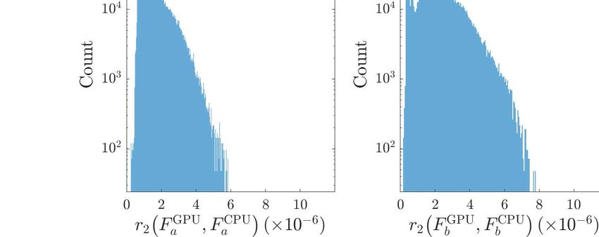
Figure 4. Histograms of the relative error in terms of the L2 norm between GPU
and CPU output for Fa (left panel ), Fb (middle panel ), and F (right panel ) for
the ComputeFstatTest tests described in section 4.2. Injected signal parameters:
(1) (k)
h0 = 1, α = 0, δ = −28◦ 48′ , f0 = 100 Hz, f0 = −10−9 Hz s−1 , f0 = 0 for k ≥ 2.
injected at 100 Hz with an unrealistically large strain h0 = 1.
ComputeFstatTest enlists three comparison metrics to compare the output for F ,
Fa , and Fb . Viewing each of F , Fa , Fb as a real (in the case of F ) or complex (in the
case of Fa and Fb ) vector with dimensionality equal to the number of frequency bins
(1000 for these tests), we compute the relative error between the GPU and CPU results
in terms of the L1 and L2 norms:
2|x − y|1,2
r1,2 (x, y) = . (9)
|x|1,2 + |y|1,2
We also compute the angle between the two vectors as
ℜ(x∗ · y)
θ = arccos , (10)
|x|2 |y|2
where x∗ · y is the usual inner product. For each set of template parameters
we confirm that these metrics do not exceed the arbitrary default tolerances in
ComputeFstatTest when comparing the existing CPU implementation of Resamp with
the GPU implementation. Histograms of the relative error between the GPU and CPU
output with the L2 norm for Fa , Fb , and F are shown in Figure 4. These show that
the L2 relative errors do not exceed ∼10−5 in these tests. For comparison, the default
tolerances in ComputeFstatTest are of the order 10−2 . The results in Figure 4 are safely
within the latter bounds. We briefly note the apparent two-peaked structure in all threeGPU F -statistic 12
panels of Figure 4. We expect that this is a numerical artifact, but we are not able to
conclusively identify a root cause for this behaviour.
5. Pilot search
In this section we apply the GPU implementation of the F -statistic to a pilot search. We
focus on the acceleration attained by the GPU implementation rather than attempting to
draw astrophysical conclusions; the design is a precursor to a future, more comprehensive
study. A full astrophysical search is outside the scope of this paper, but verifying the
utility of a GPU-accelerated F -statistic in a realistic search context is nonetheless a
valuable exercise, and that is our aim here. In Section 5.1 we describe the targets of the
pilot search. In Section 5.2 we discuss the data to be used in the search, and the choice
of search parameters. In Section 5.3 we evaluate the runtime and accuracy of the GPU
implementation under these realistic conditions, and find that the results are consistent
with those in Sections 4.1 and 4.2. Finally in Section 5.4 we discuss briefly the results
of the search.
5.1. Targets
The pilot search is a narrowband search for the four known isolated millisecond pulsars
in the globular cluster Omega Centauri (NGC 5139), PSRs J1326−4728A, C, D, and E.
These pulsars were recently discovered, in 2018 and 2019, in a radio survey undertaken at
the Parkes radio telescope following up on Australia Telescope Compact Array imaging
of the core of Omega Centauri [31]. Of the four, only PSR J1326−4728A has a complete
(1)
timing solution with a well-constrained sky position (α, δ) and spin-down rate f⋆ , but
the pulse frequency f⋆ of each pulsar is well-measured electromagneticallyk. Being newly
discovered, none of these pulsars have previously been the subject of a published directed
gravitational wave search.
Globular cluster neutron stars have been targeted in several previous searches in
LIGO data. The nearby globular cluster NGC 6544 was the subject of a directed search
for neutron stars not detected as pulsars [38]. The search was carried out on 9.2 days
of data from the sixth LIGO science run, and searched coherently with the F -statistic
(1)
over a wide range of spin-down parameters (|f0 /f0 | . 10−10 s−1 ). Known pulsars in
globular clusters have also been the subject of several targeted searches, e.g. [25, 39, 40].
In these cases the positions and spin-down parameters of the pulsars are well-measured
electromagnetically, so the parameter space which needs to be covered is small and it
is computationally feasible to use long (> 100 d) stretches of data in the search. These
targeted searches use coherent analysis methods including the F -statistic as well as the
Bayesian [41] and 5n-vector [42] methods.
The pilot search described here represents a middle ground between the above
k The subscript ⋆ refers to values intrinsic to the rotation of the star, while the subscript 0 refers to
parameters related to the gravitational wave signal at the detector, as in previous sections.GPU F -statistic 13
(1)
Pulsar f0 (Hz) f0 (Hz s−1 ) RAJ DECJ
J1326-4728A [242.88, 243.88] [−1.8, −1.4] × 10−15 13h 26m 39.7s −47◦ 30′ 11.64′′
[486.26, 487.26] [−3.6, −2.8] × 10−15 13h 26m 39.7s −47◦ 30′ 11.64′′
J1326-4728C [145.1, 146.1] [−2.8, 0.33] × 10−14 13h 26m 44s ± 7′ −47◦ 29′ 40′′ ± 7′
[290.7, 291.7] [−5.7, 0.66] × 10−14 13h 26m 44s ± 7′ −47◦ 29′ 40′′ ± 7′
J1326-4728D [217.9, 218.9] [−3.0, 0.50] × 10−14 13h 26m 44s ± 7′ −47◦ 29′ 40′′ ± 7′
[436.3, 437.3] [−6.0, 1.0] × 10−14 13h 26m 44s ± 7′ −47◦ 29′ 40′′ ± 7′
J1326-4728E [237.16, 238.16] [−3.0, 0.54] × 10−14 13h 26m 44s ± 7′ −47◦ 29′ 40′′ ± 7′
[474.8, 475.8] [−6.1, 1.1] × 10−14 13h 26m 44s ± 7′ −47◦ 29′ 40′′ ± 7′
Table 2. Search parameters for the pilot search described in Section 5. Each pair of
lines corresponds to f0 = f⋆ and 2f⋆ .
two approaches. We are searching for four known pulsars, but three of these pulsars
have unconstrained spin-down parameters and large uncertainties on their sky position,
forcing us to adopt an approach more akin to a directed search (except that the spin
frequency is well-constrained, obviating the need to search over a large number of
frequency bands). As noted above, this search is a validation exercise, whose goals
are to assess the acceleration achieved by the GPU F -statistic and its ease of use in a
practical context. It is not a full astrophysical search. Nevertheless, the selected targets
are well motivated astrophysically and could easily form part of a full search in the
future.
5.2. Data and search parameters
We perform the search using data from the second LIGO observing run (O2), which
lasted from November 30, 2016 to August 25, 2017. Strain data from the complete
run are publicly available, but we do not search using the full dataset because the
(1) 5
computational cost of a fully-coherent search over (α, δ, f0 , f0 ) scales as Tobs [43]. We
prefer to avoid including data which are of lower quality and do not contribute much to
sensitivity. As such, we perform a fully coherent search on the 100-day segment from
January 3, 2017 (GPS time 1 167 458 304) to April 13, 2017 (GPS time 1 176 098 304).
During this time both the Hanford and Livingston detectors maintained high duty
factors (fraction of time spent taking science-mode data) of 74% and 66% respectively,
compared to 59% and 57% respectively across the entirety of O2.
For each pulsar we search 1 Hz sub-bands centred on f0 = f⋆ and 2f⋆ , where
f⋆ is the pulse frequency reported by Ref. [31]. We use the default spacing between
frequency templates of 1/(2Tobs ) = 5.7 × 10⁻⁸ Hz. For those pulsars which do not have
an accurately measured position, we search over the half-power extent of the Parkes radio
telescope pointing in which the pulsars were discovered, which measures approximately
14′ × 14′ at an observing frequency of 1.4 GHz and is centred on RAJ = 13h 26m 44s ,
DECJ = −47◦ 29′ 40′′ [31].
(1)
Three of the four pulsars also do not have a well-measured spin-down rate f⋆ .GPU F -statistic 14
(1)
The observed value of f⋆ is due to both the intrinsic spin-down of the pulsar and line-
of-sight acceleration of the pulsar in the gravitational potential of the globular cluster.
(1)
The intrinsic spin-down of millisecond pulsars f∗,int is no more than −2.5 × 10⁻¹⁴ Hz s−1
for all but the brightest millisecond pulsars, with radio luminosity R1400 & 50 mJy kpc2
at 1.4 GHz [44]. PSRs J1326−4728C, D, and E are detected as relatively dim sources
with R1400 . 1.2 mJy kpc2 [31]. We therefore regard a large intrinsic spin-down as
(1)
unlikely for these pulsars, and do not consider values of f⋆,int < −2.5 × 10⁻¹⁴ Hz s−1 . A
(1)
rule of thumb for estimating the maximum apparent frequency derivative f⋆,a due to
gravitational acceleration amax is given by Ref. [45]:
(1)
f⋆,a amax 1 σ(R⊥ )2
< ≈ p , (11)
f⋆ c c rc2 + R⊥2
where R⊥ is the projected distance of the pulsar to the cluster centre, σ(R⊥ ) is the line-
of-sight velocity dispersion at R⊥ , and rc is the core radius. Given a central velocity
dispersion σ(0) = 22 km s−1 and a core radius rc = 4.6 pc [46] we set R⊥ = 0 and
estimate amax /c ≈ 1.14 × 10⁻¹⁷ s−1 . This approximation is good to ∼ 50% [45], so we
(1)
take the upper bound on |f∗,a /f | to be 2amax /c = 2.3 × 10⁻¹⁷ s−1 for safety. The range
of spin-down values to be considered for each pulsar without an existing measurement
are then obtained by combining the limits on intrinsic spindown with the limits on
spin-down due to gravitational acceleration:
2amax f⋆ 2amax f⋆
−2.5 × 10⁻¹⁴ Hz s−1 − ≤ f⋆(1) ≤ . (12)
c c
Table 2 lists the search parameters for each object. The number of sky position and
(1)
f0 templates varies between frequency bands, with bands at higher frequency requiring
more templates to cover the parameter space with a prescribed mismatch value µ. Here
we take µ = 0.1 corresponding to an upper bound on the reduction of the signal-to-noise
ratio due to template mismatch of 10%. For simplicity, the metric which controls the
template spacing is an approximate metric introduced by [43, 47], which is provided in
LALSuite. This metric accounts for modulation of the phase, but not the amplitude, of
the signal due to detector motion, in contrast to the complete metric described by [48].
As the goal of this search is only to investigate the utility of computing 2F using CUDA,
we are content to make this simplifying approximation here. The precise layout of the
templates in the parameter space is also handled by the standard LALSuite routines.
In total, 5.51 × 10⁵ sky position and spin-down templates are evaluated at 1.70 × 10⁷
frequencies each, for a total of 9.36 × 10¹² computed F -statistic values. The number of
sky position templates dominates the total number of templates: the search required
2.73 × 10⁵ sky pointings, but only 11 spin-down templates. Note that the sky pointings
and spin-down templates are not distributed evenly among the bands searched: bands
at higher f0 require more sky pointings and spin-down templates. A single spin-down
template is required for all bands except the 2f⋆ bands of PSRs J1326−4728C, D, and
E.GPU F -statistic 15
5.3. Runtime and accuracy
The search takes 17.2 GPU-hours on the same hardware as used in Section 4,
corresponding to τFeff (GPU) = 6.6 × 10⁻⁹ s. For the purpose of comparison, we run the
more expensive CPU implementation on a small subset of the parameter space covered
in the search, and find τFeff (CPU) = 4.2 × 10⁻⁷ s. Based on this value of τFeff (CPU), we
extrapolate that the pilot search would consume roughly 1092 CPU core-hours. The
overall speedup factor τFeff (CPU)/τFeff (GPU) is 64.
These timing results probe roughly the same regime as the timing measurements
shown in Figure 2 and are consistent with those results. Reading off Figure 2, we expect
τFeff (GPU) ≈ 5 × 10⁻⁹ s and τFeff (CPU) ≈ 3.5 × 10⁻⁷ s for an overall speedup factor ≈ 70.
We remind the reader that in practice the speedup of a complete search may not always
be comparable to the speedup of the computation of 2F . Once the computation of 2F
has been accelerated, other bottlenecks may emerge. For example, if every computed
2F value is to be retained on disk and/or processed further using CPU-bound code,
then the search time may be dominated by the GPU to CPU memory transfer or disk
I/O steps (see Section 4.1). These new bottlenecks may themselves be ameliorated on
a case-by-case basis (e.g. moving the CPU-bound post-processing step onto the GPU
where practical, or employing non-blocking I/O to write the results to disk).
As in Section 4.2, we verify the accuracy of the new implementation by comparison
with the existing CPU-bound implementation of the resampling algorithm. For PSRs
J1326-4728C, D, and E, we choose a 1′ ×1′ sky region at random from within the 14′ ×14′
sky region which is searched, and output all 2F values calculated with both the existing
implementation and the CUDA implementation in the first 10−3 Hz of the two frequency
bands centred on f⋆ and 2f⋆ . The sky region is chosen at random for each frequency
band. We verify that the fractional difference in 2F values does not exceed 2.5 × 10⁻⁴
and the root-mean-square fractional difference in each band does not exceed 8 × 10⁻⁶ .
These results, which we emphasise are performed on real rather than synthetic data,
are similar to those found in the Gaussian noise tests of Section 4.2.
5.4. Candidates
While we do not seek to present a full astrophysical search here, for completeness we
briefly discuss the results of the pilot search. For the purposes of this exercise, we retain
only those candidates with 2F > 70. This retention step is implemented on the GPU
side, so we do not incur the cost of transferring the full band back to the CPU and
processing it serially there. In pure Gaussian noise 2F follows a χ2 distribution with 4
degrees of freedom [24], and so the probability of at least one of the Nt = 9.36 × 10¹²
templates exceeding the 2F threshold is 1 − [Pr(2F < 70)]Nt ≈ 0.2. This is therefore
quite a conservative threshold, with a per-search false alarm probability of 20% assuming
Gaussian noise. No 2F values exceeding 70 are returned. We do not convert these non-
detections into astrophysical upper limits on the amplitude of CW signals from these
targets, as this would require expensive Monte Carlo injections which are beyond theGPU F -statistic 16
scope of this paper.
6. Discussion
We describe a new CUDA implementation for computing the F -statistic via the resampling
algorithm. The new implementation takes advantage of the power of GPUs to provide
order-of-magnitude speed-ups over the existing CPU code available in LALSuite.
The new code should not be viewed as a replacement for the existing methods.
Rather, it works alongside them, allowing F -statistic searches to take advantage of
any GPUs at their disposal. The new implementation is validated on synthetic data
with Gaussian noise. We find that the speedup with the new implementation scales
with both the observing time Tobs and the size of the frequency band ∆f , with typical
speedup factors between 10 and 100. We also verify that the CUDA implementation
remains accurate: synthetic data tests indicate that the fractional difference between the
new implementation and the existing CPU implementation does not exceed 1.5 × 10⁻⁴ .
Finally, we describe a pilot search using the new implementation on 100 days of real
data from O2. We target the four known isolated pulsars in the globular cluster
Omega Centauri, which were discovered only recently [31]. These are all millisecond
pulsars, with well-known pulse frequencies; but in three cases the spin-down frequency
is unconstrained and the position is only known to an accuracy of ±7′ , necessitating a
search over a significant number (5.51×10⁵ ) of sky position and spin-down combinations
for these targets. The search takes 17.2 GPU-hours to complete compared to a projected
45.5 CPU core-days, a speedup of ≈ 64 times. We verify that the discrepancies between
the 2F values computed by the CUDA implementation and the CPU implementation
remain small (. 2.5 × 10⁻⁴ fractionally) in real data. No detection candidates are
found. The pilot search demonstrates the utility of the new GPU implementation in
the context of a realistic search with a novel selection of targets, but we emphasise that
it is not a substitute for a full astrophysical search, which is beyond the scope of this
paper.
No effort has been made at this stage to perform optimisations in areas such as
memory layout and transfer, removing conditionals within the CUDA kernels, or searching
several templates simultaneously in cases where the GPU’s capability is not saturated
by the computation required for a single template. The work reported here represents
a first pass at the problem, with room for further optimisation in the future.
Beyond further optimisation, we briefly mention two other avenues for future
work. One is the comparison of this implementation with two other in-development
implementations of the F -statistic which employ CUDA¶ and OpenCL+ (M. Bejger, private
communication). Another is investigating whether this work can be used to speed up the
resampling implementation [49] of the CrossCorrelation search for gravitational waves
from sources in binary systems.
¶ https://github.com/mbejger/polgraw-allsky/tree/master/search/network/src-gpu
+
https://github.com/MathiasMagnus/polgraw-allsky/tree/d36f9c238b76c2d683db393ee1cc34a2a3100bf1/search/nGPU F -statistic 17
In [50] we perform an all-sky search for continuous gravitational waves over a 1 Hz
frequency band, pursuing a strategy of maximising sensitivity over a narrow parameter
domain. The search uses a semi-coherent search algorithm [51–53]; data from O2 are
partitioned into segments of duration ∼ 10 d, each segment is searched using the F -
statistic, and results from all segments are then summed together. GPUs are used to
compute the F -statistic for each segment, using the implementation presented here, as
well as the sum over segments. The search achieves a sensitivity of h0 = 1.01 × 10⁻²⁵
and is limited by available computational resources. We estimate that, without
the computational speed-up from the GPU F -statistic implementation, but with the
same limited computational resources, the sensitivity achieved after re-configuring the
parameters of the search (number of segments, segment length, template placement,
and frequency band) would have been reduced by ∼ 8%. For example, the segment
length would have been shortened to ∼ 5.5 d to reduce the computational cost of the F -
statistic. The modest difference in sensitivity, with and without the speed-up from the
GPU F -statistic implementation, is ultimately due to the shallow scaling of sensitivity
with computational cost for semi-coherent algorithms [54]. However, it is still significant
scientifically, in situations where sound astrophysical arguments exist (e.g. indirect spin-
down limits) that plausible sources are emitting near the detection limits of current
searches [55].
Acknowledgments
We thank David Keitel for helpful comments on the manuscript. This research is
supported by the Australian Research Council Centre of Excellence for Gravitational
Wave Discovery (OzGrav) through project number CE170100004. This work was
performed on the OzSTAR national facility at Swinburne University of Technology.
OzSTAR is funded by Swinburne University of Technology and the National
Collaborative Research Infrastructure Strategy (NCRIS).
References
[1] Riles K 2017 Modern Physics Letters A 32 1730035–1730685 (Preprint 1712.05897)
[2] Aasi J et al. 2015 Classical and Quantum Gravity 32 74001 (Preprint 1411.4547)
[3] Acernese F et al. 2015 Classical and Quantum Gravity 32 24001 ISSN 0264-9381 (Preprint
1408.3978)
[4] Akutsu T et al. (KAGRA Collaboration) 2019 Nature Astronomy 3 35–40 ISSN 2397-3366
(Preprint 1811.08079)
[5] Abbott B P et al. 2016 Physical Review Letters 116 241103 (Preprint 1606.04855)
[6] Abbott B P et al. 2017 Physical Review Letters 119 161101 (Preprint 1710.05832)
[7] Dergachev V and Papa M A 2021 Physical Review D 104 043003 (Preprint 2104.09007)
[8] Abbott R, Abbott T D, Abraham S, Acernese F, Ackley K, Adams A, Adams C, Adhikari R X,
Adya V B, Affeldt C and et al 2021 Physical Review D 104 082004
[9] Ashok A, Beheshtipour B, Alessandra Papa M, Freire P C C, Steltner B, Machenschalk B, Behnke
O, Allen B and Prix R 2021 arXiv e-prints arXiv:2107.09727 (Preprint 2107.09727)GPU F -statistic 18
[10] Abbott R, Abbott T D, Abraham S, Acernese F, Ackley K, Adams A, Adams C, Adhikari R X,
Adya V B, Affeldt C and et al 2020 The Astrophysical Journal Letters 902 L21 (Preprint
2007.14251)
[11] Nvidia Corporation 2019 CUDA Toolkit Documentation URL https://docs.nvidia.com/cuda/
[12] Stone J E, Gohara D and Shi G 2010 Computing in Science & Engineering 12 66–73 ISSN 1521-
9615
[13] Liu Y, Du Z, Chung S K, Hooper S, Blair D and Wen L 2012 Classical and Quantum Gravity 29
235018 ISSN 2649381
[14] Guo X, Chu Q, Chung S K, Du Z, Wen L and Gu Y 2018 Computer Physics Communications 231
62–71 ISSN 104655
[15] Talbot C, Smith R, Thrane E and Poole G B 2019 Physical Review D 100 43030 ISSN 2470-0010
(Preprint 1904.02863)
[16] Wysocki D, O’Shaughnessy R, Lange J and Fang Y L L 2019 Physical Review D 99 84026 ISSN
2470-0010 (Preprint 1902.04934)
[17] Keitel D and Ashton G 2018 Classical and Quantum Gravity 35 205003 (Preprint 1805.05652)
[18] Abbott B P et al. (LIGO Scientific Collaboration and Virgo Collaboration and others) 2019
Physical Review D 100 122002 URL https://doi.org/10.1103/PhysRevD.100.122002
[19] Astone P, Colla A, D’Antonio S, Frasca S and Palomba C 2014 Physical Review D 90 042002
(Preprint 1407.8333)
[20] La Rosa I, Astone P, D’Antonio S, Frasca S, Leaci P, Miller A L, Palomba C, Piccinni O J, Pierini
L and Regimbau T 2021 Universe 7 218
[21] George D and Huerta E A 2018 Physical Review D 97 044039 (Preprint 1701.00008)
[22] Gabbard H, Williams M, Hayes F and Messenger C 2018 Physical Review Letters 120(14) 141103
[23] Dreissigacker C, Sharma R, Messenger C, Zhao R and Prix R 2019 Physical Review D 100 44009
ISSN 2470-0010
[24] Jaranowski P, Królak A and Schutz B F 1998 Physical Review D 58(6) 063001
[25] Abbott B P et al. 2019 The Astrophysical Journal 879 10 (Preprint 1902.08507)
[26] Abbott B P et al. 2019 Physical Review D 100 024004 (Preprint 1903.01901)
[27] LIGO Scientific Collaboration 2018 LIGO Algorithm Library - LALSuite free software (GPL)
[28] Prix R 2011 The F-statistic and its implementation in ComputeFStatistic v2 Tech. Rep. LIGO-
T0900149-v6 LIGO URL https://dcc.ligo.org/LIGO-T0900149-v6/public
[29] Williams P R and Schutz B F 2000 An efficient matched filtering algorithm for the detection of
continuous gravitational wave signals AIP Conference Series vol 523 ed Meshkov S (Melville:
American Institute of Physics) pp 473–476
[30] Patel P, Siemens X, Dupuis R and Betzwieser J 2010 Physical Review D 81 84032 ISSN 1550-7998
(Preprint 0912.4255)
[31] Dai S, Johnston S, Kerr M, Camilo F, Cameron A, Toomey L and Kumamoto H 2020 The
Astrophysical Journal 888 L18 ISSN 2041-8205
[32] Prix R and Krishnan B 2009 Classical and Quantum Gravity 26 204013 ISSN 0264-9381, 1361-6382
(Preprint 0907.2569)
[33] Press W H, Teukolsky S A, Vetterling W T and Flannery B P 2007 Numerical Recipes 3rd Edition:
The Art of Scientific Computing 3rd ed (New York, NY, USA: Cambridge University Press)
ISBN 0521880688, 9780521880688
[34] Suvorova S, Sun L, Melatos A, Moran W and Evans R J 2016 Physical Review D 93 ISSN 15502368
(Preprint 1606.02412)
[35] Abbott B P et al. 2017 Physical Review D 95 122003 ISSN 2470-0010 (Preprint 1704.03719)
[36] Suvorova S, Clearwater P, Melatos A, Sun L, Moran W and Evans R J 2017 Physical Review D
96 102006 ISSN 2470-0010 (Preprint 1710.07092)
[37] Prix R 2017 Characterizing timing and memory-requirements of the F -statistic
implementations in LALSuite Tech. Rep. LIGO-T1600531-v4 LIGO URL
https://dcc.ligo.org/LIGO-T1600531/publicGPU F -statistic 19
[38] Abbott B P 2017 Physical Review D 95 082005 (Preprint 1607.02216)
[39] Abbott B P 2010 The Astrophysical Journal 713 671–685 (Preprint 0909.3583)
[40] Aasi J 2014 The Astrophysical Journal 785 119 (Preprint 1309.4027)
[41] Dupuis R J and Woan G 2005 Physical Review D 72 102002 (Preprint gr-qc/0508096)
[42] Astone P, D’Antonio S, Frasca S and Palomba C 2010 Classical and Quantum Gravity 27 194016
ISSN 0264-9381
[43] Brady P R, Creighton T, Cutler C and Schutz B F 1998 Physical Review D 57 2101–2116
[44] Manchester R N, Hobbs G B, Teoh A and Hobbs M 2005 The Astronomical Journal 129 1993–1993
[45] Phinney E S 1992 Philosophical Transactions: Physical Sciences and Engineering 341 39–75 ISSN
0962-8428
[46] Meylan G, Mayor M, Duquennoy A and Dubath P 1995 Astronomy and Astrophysics 303 761
ISSN 0004-6361
[47] Whitbeck D 2006 Observational Consequences of Gravitational Wave Emission From
Spinning Compact Sources Ph.D. thesis The Pennsylvania State University URL
https://etda.libraries.psu.edu/paper/7132/
[48] Prix R 2007 Physical Review D 75 023004 (Preprint gr-qc/0606088)
[49] Meadors G D, Krishnan B, Papa M A, Whelan J T and Zhang Y 2018 Physical Review D 97 ISSN
24700029
[50] Wette K, Dunn L, Clearwater P and Melatos A 2021 Physical Review D 103(8) 083020 URL
https://doi.org/10.1103/PhysRevD.103.083020
[51] Wette K and Prix R 2013 Physical Review D 88 123005 (Preprint 1310.5587) URL
https://doi.org/10.1103/PhysRevD.88.123005
[52] Wette K 2015 Physical Review D 92 082003 ISSN 1550-2368 (Preprint 1508.02372) URL
https://doi.org/10.1103/PhysRevD.92.082003
[53] Wette K, Walsh S, Prix R and Papa M A 2018 Physical Review D 97 123016 (Preprint 1804.03392)
URL https://doi.org/10.1103/PhysRevD.97.123016
[54] Prix R and Shaltev M 2012 Physical Review D 85 084010 (Preprint 1201.4321) URL
https://doi.org/10.1103/PhysRevD.85.084010
[55] Riles K 2013 Progress in Particle and Nuclear Physics 68 1–54 (Preprint 1209.0667)You can also read