Global Earth Magnetic Field Modeling and Forecasting with Spherical Harmonics Decomposition - arXiv
←
→
Page content transcription
If your browser does not render page correctly, please read the page content below
Global Earth Magnetic Field Modeling and
                                                 Forecasting with Spherical Harmonics Decomposition

                                                               Panagiotis Tigas∗                      To Bloch∗                        Vishal Upendran∗
arXiv:2102.01447v1 [physics.geo-ph] 2 Feb 2021

                                                                   OATML                         University of Reading                     IUCAA
                                                              University of Oxford                   Reading, UK                          Pune, India
                                                                  Oxford, UK

                                                             Banafsheh Ferdoushi∗                       Yarin Gal                     Siddha Ganju
                                                          University of New Hampshire                    OATML                     NVIDIA Corporation
                                                              Durham, NH, USA                       University of Oxford           Santa Clara, CA, USA
                                                                                                        Oxford, UK

                                                         Ryan M. McGranaghan                   Mark C. M. Cheung                           Asti Bhatt
                                                              ASTRA LLC                          Lockheed Martin                        SRI International
                                                          Louisville, CO, USA               Advanced Technology Center                 Menlo Park, CA, USA
                                                                                               Palo Alto, CA, USA

                                                                                                     Abstract

                                                              Modeling and forecasting the solar wind-driven global magnetic field perturbations
                                                              is an open challenge. Current approaches depend on simulations of computationally
                                                              demanding models like the Magnetohydrodynamics ( MHD ) model or sampling
                                                              spatially and temporally through sparse ground-based stations ( SuperMAG ). In
                                                              this paper, we develop a Deep Learning model that forecasts in Spherical Harmonics
                                                              space 2 , replacing reliance on MHD models and providing global coverage at one-
                                                              minute cadence, improving over the current state-of-the-art which relies on feature
                                                              engineering. We evaluate the performance in SuperMAG dataset (improved by
                                                              14.53%) and MHD simulations (improved by 24.35%). Additionally, we evaluate
                                                              the extrapolation performance of the spherical harmonics reconstruction based on
                                                              sparse ground-based stations ( SuperMAG ), showing that spherical harmonics can
                                                              reliably reconstruct the global magnetic field as evaluated on MHD simulation.

                                                 1       Introduction
                                                 The space environment around Earth (geospace) does not exist in a steady state. The dynamical
                                                 changes in geospace is termed space weather. Space weather is primarily driven by interactions
                                                 between the Sun’s output (in terms of solar radiation and the magnetized solar wind) with the
                                                 Earth’s magnetosphere, thermosphere and ionosphere. The US National Oceanic and Atmospheric
                                                 Administration continuously monitors the solar wind upstream from Earth with satellite observatories
                                                 orbiting Lagrangian point L1 along the Sun-Earth line. The solar wind energy is transferred to the
                                                 Earth’s magnetosphere via complex mechanisms [Dungey, 1961], leading to perturbations in the
                                                 Earth’s magnetic field called geomagnetic storms.
                                                     ∗
                                                         equal contribution
                                                     2
                                                         We will release all the code and models used in this work post-publication.

                                                 Third Workshop on Machine Learning and the Physical Sciences (NeurIPS 2020), Vancouver, Canada.
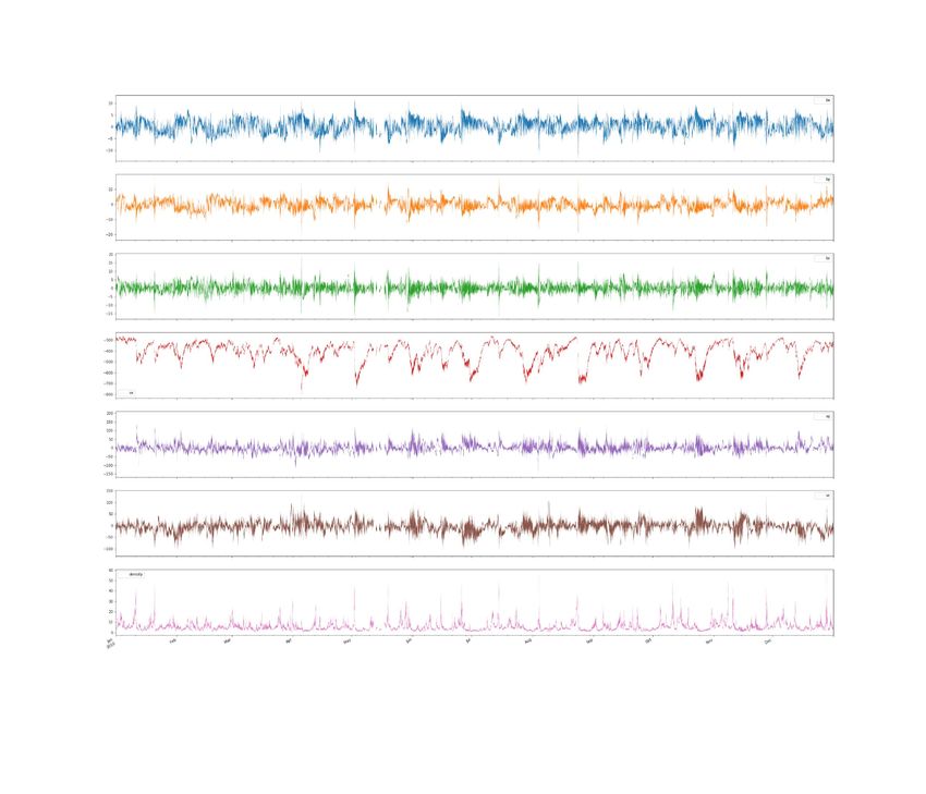
Solar wind
    parameters

                                                                                               Sampled
                                                                       Predictions
                                                                                              Predictions

Figure 1: Model architecture. Solar Wind data are summarized into an embedding vector using
a Gated Recurrent Unit (GRU) which is then passed to a Multilayer Perceptron (MLP) to output
the predicted spherical harmonics coefficients from where we can extrapolate values for specific
locations.

Geomagnetic storms drive a spectrum of potentially catastrophic disruptions to our technologically-
dependent society, among the most threatening being critical disturbances to the electrical grid in the
form of geomagnetically induced currents ( GICs ). Due to their proprietary nature, publicly available
 GIC data are limited. However, a cohort study of insurance claims of electrical equipment provides
evidence that space weather poses a continuous threat to electrical distribution grids via geomagnetic
storms and GICs [Schrijver et al., 2014, Eastwood et al., 2018]. GICs also pose threats to oil
pipelines, railyways and telecommunication systems. In the case of extreme, but historically probable
geomagnetic storms, the economic impact due to prolonged power outages can exceed billions of
dollars per day [Oughton et al., 2017]. For this reason, there is urgency among public and industry
stakeholders to improve monitoring and forecasting of space weather impacts like geomagnetic
storms and GICs .
The geomagnetic field is continuously monitored, importantly with sparse spatial coverage, by a
network of roughly 200 ground magnetometers [Gjerloev, 2012b] and by a constellation of 66
satellites collectively known as the Active Magnetosphere and Planetary Electrodynamics Response
Experiment ( AMPERE ) project [AMPERE; Waters et al., 2020] in low Earth orbit. The spatially-
sparse magnetometer measurements are typically synthesized into global indices (e.g. Dst, Kp, and
AE ; see appendix for more details) as measures of the geoeffectiveness of space weather perturbations.
Like most indices, they are good as indicators but are too far removed from the underlying governing
equations of the system. This makes interpretability and forecasting (whether by physics-based or
physics-agnostic ML models) difficult.
GICs are driven by geoelectric fields through Ohms law, J~ = σ E     ~ (the displacement current is
                     ~
negligible), where J is the current, σ the conductivity tensor, and E   ~ is the electric field. The
geoelectric field is related to the ground magnetic field perturbations through the Faradays law
of induction −∇ × E   ~ = ∂ B~ , where, ∂ B~ is the rate of change of magnetic field on the Earth’s
                             ∂t          ∂t
surface and can be derived from the time derivative of magnetic perturbation based on ground Earth
magnetometers.
Our contributions are:
       1. Using simulation data from a physics-based ( MHD ) model to validate a compressed sensing
          technique to recover global maps (in spherical harmonic basis) of the geomagnetic perturba-
          tion from sparse measurements. This improves the temporal cadence of such maps by >10x.

       2. Developing a Deep Learning model that operates in the spherical harmonics space, allowing
          for global modeling of the magnetic field disturbances, combined with powerful non-linear
          autoregressive models (RNN, 1D-CNN) to capture the influence of solar wind data.

2    Datasets
We used data describing Earth’s magnetosphere and solar wind properties between 1 Jan 2013
and 31 Dec 2013. We used OMNI dataset for solar wind data, which captures the interplanetary
magnetic field components (IMF), velocity and temperature of the solar wind as well as the clock

                                                  2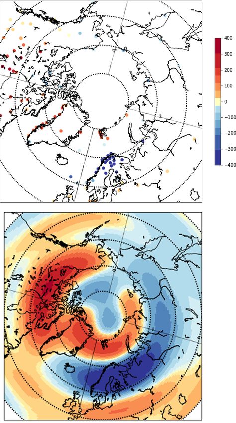
angle. 3 . For Earth’s magnetic field, we used SuperMAG dataset [Gjerloev, 2012a] which consists
of geomagnetic perturbations measurements from ground earth stations located at various places
around the globe.
Finally, we used a simulation-derived dataset based on simulations conducted with Open Geospace
General Circulation Model ( Open GGCM ) [Raeder et al., 2001], a magnetohydrodynamics ( MHD )
model. Lacking a global and spatially-complete ground-based magnetometer array we must rely on
the first principles MHD model to constitute a global ground truth dataset. Furthermore, this allows
us to validate our approach on finer resolution than one supported by SuperMAG and AMPERE
dataset. However, note that the MHD model is not a substitute for actual perturbation measurements,
for many short-scale phenomena are missed by such models [Raeder et al., 2001].

3         Methodology
In order to properly forecast GICs, we need to be able to model the relationship between the solar
wind parameters and interplanetary magnetic fields (IMF) with the Earth system. Due to the scarcity
of GIC data, the comparatively abundant magnetometer data and the relationship between the two, a
                                               ~
logical step is to create models to predict ∂∂tB . Such models provide complete spatial coverage and
permit the study of the nature of the connection between the solar wind and the Earth.

3.1       Spherical Harmonics Decomposition

Any scalar field over the unit sphere can be expressed as f (θ, φ) =
P ∞ Pn
  n=0   m=−n anm Ynm (θ, φ), where
                        s
                          2n + 1 (n − m)! imθ m
         Ynm (θ, φ) :=                    e Pn (cos(φ)),
                            4π (n + m)!

 and Pnm (cos(φ)) are the associated Legendre polynomials. These functions
Ynm (θ, φ) are solutions to Laplace equation in a 3-D spherically symmetric
coordinate system. If the sum is truncated at maximum harmonic degree
                                             PN Pn
N , f (θ, φ) is approximated as f˜(θ, φ) = n=0 m=−n anm Ynm (θ, φ).
Defining i = n2 + n + m, the double sum can be written as f˜(θ, φ) =
P(N +1)2 −1
   i=0        ai Yi (θ, φ). If the 2D fields over θ, φ are unrolled as one-
dimensional arrays, we have f˜ = B~a, where ~a = (ai ) is the tuple of
spherical harmonic coefficients, and B = (~bi ) is the basis matrix wherein
column vector ~bi represents the basis function Ynm (θ, φ).

3.2       Experimental Design
                                                                               Figure 2: Ground truth
3.2.1      Reconstruction                                                      observations (top) and
                                                                               Spherical harmonic re-
With SuperMAG data, we have spatially sparse samples y which can be construction (bottom)
any component of the geomagnetic field, or its deviation from a reference of dbn_nez.
field) measured at 2̃00 stations. Note that only the Northern Hemisphere
is considered in this analysis, for it has an extensive coverage (in contrast to the extremely sparse
coverage in the Southern Hemisphere). The spherically symmetric reconstruction thus is f˜(θ, φ),
and this reconstruction as evaluated at the station locations is ỹ. Thus, we first construct a set of
coefficients ~a from this sparse set of measurements, considered all the measurements across the globe
at each time step. There are two constraints imposed for obtaining the set of coefficients:
          1. The coefficient set must be sparse: This is to prevent power leakage and coupling across
             multiple modes.
      3
    Solar wind measurement is performed by ACE and WIND satellites at the L1 Lagrange point of the
Sun-Earth system

                                                    3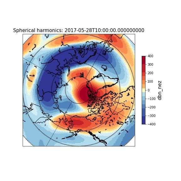
2. As small N as possible: Since, in theory, an infinite number of modes can fit the observations,
           but a parsimonious model is required to limit overfitting. Furthermore, we would not want
           unnatural, localized artifacts due to high number of modes, thereby motivating a constraint
           on n.
To mitigate constraint (1), we apply a Lasso regression technique [Tibshirani, 1996] with the spherical
harmonic functions as the basis.
The Lasso regression comes with
a regularization term αk~ak1 , where
k~ak1 is the L1-norm of the coeffi-
cients and α > 0 is a hyperparame-
ter. This, and constraint (2) are miti-
gated by varying both α and the maxi-
mum number of modes N , and search-
ing for a knee in a defined error met-
ric, subject to the smallest maximum Figure 3: L1 error (left) and R2 (right) "knee" determination.
modes. The sweep parameters are de-
tailed in Table. 2, and two metrics are used – Maximum L1 error across all stations and time, and
maximum R2 metric (coefficient of determination) across all time steps. The maximum L1 error tells
us the worst performance across the dataset, and thus we seek the most acceptable worst possible
performance. As shown in Fig. 3, the "knee of goodness" can be seen corresponding to α = 0.1, and
20 maximum modes. These parameters are fixed in our analysis.
An example reconstruction of the data from 2017, considering stations above 40◦ is shown in Fig. 2.
Here, we compare the north facing component of ∂d/∂t from SuperMAG and its reconstruction.
Similarly, the comparison of spherical harmonic reconstruction for the MHD simulation is shown in
Fig. 4. Note here, that the reconstruction is performed by sampling the MHD simulation at locations
of SuperMAG stations alone.

3.2.2    Forecasting
Next, we construct a forecasting model which uses solar wind data ( OMNI ) to forecast the global
magnetic field perturbation. For this experiment we use a similar setup as Weimer [2013] model . We
feed 25 minutes of solar wind activity into a Gated Recurrent Network (GRU) to map the sequence
into an embedding vector. We then feed the embedding into a Multilayer Perceptron (MLP) to output
the spherical harmonics coefficients which model the global magnetic field perturbation; specifically
we focus on north component of ∂d/∂t as a proof of concept. In contrast to Weimer [2013] model ,
we use the whole sequence as input to a non-linear autoregressive model and we do not apply feature
engineering to the OMNI data. Instead we use the raw features (see appendix for detailed list of
features). The architecture can be seen in fig. 1.
We benchmark this work against the state-of-the-art empirical model by Wiemer et al. [Weimer,
2013]. To evaluate the performance we first compare on the validation set on SuperMAG but also we
compare on simulations conducted with MHD model for two weeks worth of activity. The results are
summarized in table 1.

4   Results And Discussion
                                Table 1: Forecasting model performance
             Model                      SuperMAG (val) RMS (nT) ↓          MHD RMS (nT) ↓
             Ours.                                               24.23                 27.02
             Weimer [2013] model                                 28.35                 35.72

With this work, we show and evaluate the reconstruction of the global magnetic perturbation field using
spherical harmonics with LASSO regularization to promote sparsity in the coefficients. We show that
it is possible to reconstruct from sparse measurements like the ones provided by SuperMAG stations,

                                                     4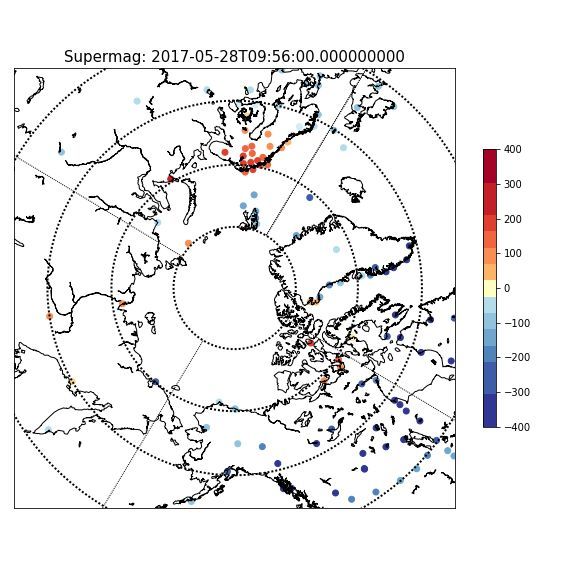
Figure 4: Comparison of reconstruction with the MHD simulation. Left: MHD simulation; center:
MHD simulation sampled at SuperMAG station locations; right: Reconstruction.

and we evaluated on MHD data to show that the reconstruction is similar to the global field modeled
by MHD , suggesting that the results of such models can be compressed in spherical harmonics space
by compressed sensing techniques. Additionally, we show that by using a Deep Neural Network
to forecast in the spherical harmonics space, we can improve over existing state of the art (Weimer
[2013] model ) by 14.53% on SuperMAG and 24.35% on MHD dataset (summarized in table 1).

Broader Impact
Geomagnetic storms drive a spectrum of potentially catastrophic disruptions to our technologically-
dependent society, among the most threatening being critical disturbances to the electrical grid in the
form of geomagnetically induced currents ( GICs ). Due to their proprietary nature, publicly available
 GIC data are limited. However, a cohort study of insurance claims of electrical equipment provides
evidence that space weather poses a continuous threat to electrical distribution grids via geomagnetic
storms and GICs [Schrijver et al., 2014, Eastwood et al., 2018]. GICs also pose threats to oil
pipelines, railways and telecommunication systems. In the case of extreme, but historically probable
geomagnetic storms, the economic impact due to prolonged power outages can exceed billions of
dollars per day [Oughton et al., 2017]. For this reason, there is urgency among public and industry
stakeholders to improve monitoring and forecasting of space weather impacts like geomagnetic
storms and GICs . With this work, we progress towards better and faster forecasting models which
will help us shield our infrastructure from solar-wind related hazards.

Acknowledgments and Disclosure of Funding
This project was conducted during the 2020 NASA Frontier Development Lab (FDL) program, a
public-private partnership between NASA, the SETI Institute, and commercial partners. We wish
to thank, in particular, NASA, Google Cloud, NVIDIA, Intel and SRI, for supporting this project.
Finally, we gratefully acknowledge the SuperMAG collaborators.

References
J. W. Dungey. Interplanetary magnetic field and the auroral zones. Physical Review Letters, 6(2):47,
   1961.

J. Eastwood, M. Hapgood, E. Biffis, D. Benedetti, M. Bisi, L. Green, R. Bentley, and C. Burnett.
   Quantifying the economic value of space weather forecasting for power grids: An exploratory
   study. Space weather, 16(12):2052–2067, 2018.

J. Gjerloev. The supermag data processing technique. Journal of Geophysical Research: Space
   Physics, 117(A9), 2012a.

J. W. Gjerloev. The SuperMAG data processing technique. Journal of Geophysical Research: Space
   Physics, 117(A9), 2012b. ISSN 2156-2202. doi: 10.1029/2012JA017683.

                                                  5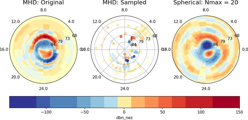
E. J. Oughton, A. Skelton, R. B. Horne, A. W. P. Thomson, and C. T. Gaunt. Quantifying the daily
   economic impact of extreme space weather due to failure in electricity transmission infrastructure.
  Space Weather, 15(1):65–83, Jan. 2017. doi: 10.1002/2016SW001491.
J. Raeder, Y. Wang, and T. J. Fuller-Rowell. Geomagnetic storm simulation with a coupled
   magnetosphere-ionosphere-thermosphere model. Space weather, 125:377–384, 2001.
C. J. Schrijver, R. Dobbins, W. Murtagh, and S. M. Petrinec. Assessing the impact of space weather
  on the electric power grid based on insurance claims for industrial electrical equipment. Space
  Weather, 12(7):487–498, July 2014. doi: 10.1002/2014SW001066.
R. Tibshirani. Regression shrinkage and selection via the lasso. Journal of the Royal Statistical
  Society: Series B (Methodological), 58(1):267–288, 1996.
C. L. Waters, B. J. Anderson, D. L. Green, H. Korth, R. J. Barnes, and H. Vanhamäki. Science Data
  Products for AMPERE, volume 17, page 141. 2020. doi: 10.1007/978-3-030-26732-2_7.
D. R. Weimer. An empirical model of ground-level geomagnetic perturbations. Space Weather-the
  International Journal of Research and Applications, 11(3):107–120, 2013.

                                                  6
A Reconstruction experiment sweep parameter
Table 2: Sweep parameter description for reconstruction
Sweep parameter Description
Date range 2015-06-23 to 2015-06-24
Cadence 10 min
Max modes sweep [5,50], steps of 5
α sweep {2,1,0.1,1e-3,1e-5}
Max L1 metric maxstations maxPtime ||y − ỹ||1
Max R2 score maxtime (1 − stations |y − ỹ|1 /variance(y))
Note that we have used a cadence of 10 min for quick computation of the metrics over the dataset –
however, since the spherical harmonic generation is done at each time step, it can be performed at
whatever cadence necessary.
B Solar Wind Data - OMNI Dataset
Here we describe the features we used from OMNI Dataset.
Table 3: Description of OMNI Dataset features
Feature Description
q
BT : Magnetic field magnitude ( (Bx2 + By2 ))
q
VSW : Solar Wind velocity magnitude ( (Vx2 + Vy2 + Vz2 ))
T: Temperature of the solar wind
θc : Clock angle of the interplanetary magnetic field (IMF)
F10.7 : F10.7 measures the noise level generated by the sun at a wavelength of 10.7 cm.
C Geoeffectieness Indices
Dst: (Disturbance Storm Time Index) It is the measure of geomagnetic activity derived from near
equator ground magnetic stations providing information about the strength of ring current.
Kp: Global geomagnetic index that is based on 3 hour measurements of mid-latitude ground magnetic
stations around the world.
AE: (Auroral Electrojet Index) It is the measure of auroral activity determined based on ground
magnetic stations around aurora zone.
D Weimer [2013] model
Weimer [2013] model baseline model is designed to forecast each of the three magnetic vector
components. It uses solar wind data as input and it outputs the spherical harmonics coefficients,
which then can be used to extract the forecasting values per CGM latitude and MLT pair.
A feature vector from the solar wind data is derived
71
BT
VSW
p t
(F10.7 )
BT cos(θc )
VSW cos(θc )
t
p cos(θc )
F = , (1)
(F10.7 ) cos(θc )
B sin(θ )
T c
VSW sin(θc )
p t sin(θc )
(F10.7 ) sin(θc )
BT cos(2θc )
VSW cos(2θc )
BT sin(2θc )
VSW sin(2θc )
p
where BT represents the magnitude of the magnetic field, VSW the solar wind velocity, (F10.7 )
the square root of the F 10.7 feature (a measure of solar radiation), t the dipole axis angle in radians
and θc the clock angle.
Weimer [2013] model is trained on data obtained from SuperMAG stations for the year 2013 with
the loss MSE = Avg((y − Ba)2 ), where a are the spherical harmonics coefficients, computed as
m
am
n = ( gn , hm
n )
|{z} |{z}
Real Part Imaginary Part
The coefficients are computed as gnm = Gm m m m m
n F and hn = Hn F , where Gn and Hn are the weights
to learn.
The model is trained on 25 minute long average of solar wind data, with a lag of 20 minutes and as
target the magnetic field perturbation of 5 minutes long averages, as measured by SuperMAG stations.
E Reproducibility details of forecasting experiments
The model architecture used for the forecasting experiment is presented below. The model was
trained using Adam optimizer with learning rate lr=1e-04 and Mean Squared Error as a loss.
class GeoeffectiveNet(nn.Module):
def __init__(self,
past_omni_length,
future_length,
omni_features,
supermag_features,
nmax,
targets):
super(GeoeffectiveNet, self).__init__()
self.omni_past_encoder = nn.GRU(25,
16,
num_layers=1,
bidirectional=False,
batch_first=True,
dropout=0.5)
n_coeffs = 0
8for n in range(nmax+1):
for m in range(0, n+1):
n_coeffs += 1
n_coeffs *= 2
self.encoder_mlp = nn.Sequential(
nn.Linear(16, 16),
nn.ELU(inplace=True),
nn.Dropout(p=0.5),
nn.Linear(16, n_coeffs, bias=False) # 882
)
self.omni_features = omni_features
self.supermag_features = supermag_features
self.targets = targets
self.future_length = future_length
def forward(self,
past_omni,
past_supermag,
future_supermag,
dates,
future_dates,
**kargs):
past_omni = NamedAccess(past_omni, self.omni_features)
features = []
# add the wiemer2013 features
bt = (past_omni['by']**2 + past_omni['bz']**2)**.5
v = (past_omni['vx']**2 + past_omni['vy']**2 + past_omni['vz']**2)**.5
features.append(past_omni['bx'])
features.append(past_omni['by'])
features.append(past_omni['bz'])
features.append(bt)
features.append(v)
features.append(past_omni['dipole'])
features.append(torch.sqrt(past_omni['f107']))
features.append(bt*torch.cos(past_omni['clock_angle']))
features.append(v*torch.cos(past_omni['clock_angle']))
features.append(past_omni['dipole']*torch.cos(past_omni['clock_angle']))
features.append(torch.sqrt(past_omni['f107'])*torch.cos(past_omni['clock_angle']))
features.append(bt*torch.sin(past_omni['clock_angle']))
features.append(v*torch.sin(past_omni['clock_angle']))
features.append(past_omni['dipole']*torch.sin(past_omni['clock_angle']))
features.append(torch.sqrt(past_omni['f107'])*torch.sin(past_omni['clock_angle']))
features.append(bt*torch.cos(2*past_omni['clock_angle']))
features.append(v*torch.cos(2*past_omni['clock_angle']))
features.append(past_omni['dipole']*torch.cos(2*past_omni['clock_angle']))
features.append(torch.sqrt(past_omni['f107'])*torch.cos(2*past_omni['clock_angle']))
features.append(bt*torch.sin(2*past_omni['clock_angle']))
features.append(v*torch.sin(2*past_omni['clock_angle']))
features.append(past_omni['dipole']*torch.sin(2*past_omni['clock_angle']))
9features.append(torch.sqrt(past_omni['f107'])*torch.sin(2*past_omni['clock_angle']))
features.append(past_omni['clock_angle'])
features.append(past_omni['temperature'])
features = torch.stack(features, -1)
encoded = self.omni_past_encoder(features)[1][0]
coeffs = self.encoder_mlp(encoded)
predictions = torch.einsum('bij,bj->bi', future_supermag.squeeze(1), coeffs)
return coeffs, predictions, None
For the spherical harmonics decomposition we used scipyṡpecialṡph_harm function.
def basis_matrix(nmax, theta, phi):
from scipy.special import sph_harm
assert(len(theta) == len(phi))
basis = []
for n in range(nmax+1):
for m in range(-n,n+1):
y_mn = sph_harm(m, n, theta, phi)
basis.append(y_mn.real.ravel())
basis.append(y_mn.imag.ravel())
basis = np.array(basis)
return basis
.reshape(-1, theta.shape[0], theta.shape[1])
.swapaxes(0, 1).swapaxes(2, 1)
F International Geomagnetic Reference Field
IGRF( International Geomagnetic Reference Field): Empirical measurements of the Earth magnetic
field representing the main field without external sources.
10You can also read