GEOMETRY MATTERS: EXPLORING LANGUAGE EXAM- PLES AT THE DECISION BOUNDARY
←
→
Page content transcription
If your browser does not render page correctly, please read the page content below
Under review as a conference paper at ICLR 2021

                                        G EOMETRY  MATTERS : E XPLORING LANGUAGE EXAM -
                                        PLES AT THE DECISION BOUNDARY

                                         Debajyoti Datta, Shashwat Kumar, Laura Barnes                    Tom Fletcher
                                         Systems Engineering                                              Department of Computer Science
                                         University of Virginia                                           University of Virginia
                                         {dd3ar,sk9epp,lb3dp}@virginia.edu                                ptf8v@virginia.edu

                                                                                      A BSTRACT
arXiv:2010.07212v2 [cs.CL] 6 Dec 2020

                                                 A growing body of recent evidence has highlighted the limitations of natural
                                                 language processing (NLP) datasets and classifiers. These include the presence
                                                 of annotation artifacts in datasets, classifiers relying on shallow features like a
                                                 single word (e.g., if a movie review has the word “romantic”, the review tends
                                                 to be positive), or unnecessary words (e.g., learning a proper noun to classify a
                                                 movie as positive or negative). The presence of such artifacts has subsequently
                                                 led to the development of challenging datasets to force the model to generalize
                                                 better. While a variety of heuristic strategies, such as counterfactual examples
                                                 and contrast sets, have been proposed, the theoretical justification about what
                                                 makes these examples difficult for the classifier is often lacking or unclear. In
                                                 this paper, using tools from information geometry, we propose a theoretical way
                                                 to quantify the difficulty of an example in NLP. Using our approach, we explore
                                                 difficult examples for several deep learning architectures. We discover that both
                                                 BERT, CNN and fasttext are susceptible to word substitutions in high difficulty
                                                 examples. These classifiers tend to perform poorly on the FIM test set. (generated
                                                 by sampling and perturbing difficult examples, with accuracy dropping below 50%).
                                                 We replicate our experiments on 5 NLP datasets (YelpReviewPolarity, AGNEWS,
                                                 SogouNews, YelpReviewFull and Yahoo Answers). On YelpReviewPolarity we
                                                 observe a correlation coefficient of -0.4 between resilience to perturbations and the
                                                 difficulty score. Similarly we observe a correlation of 0.35 between the difficulty
                                                 score and the empirical success probability of random substitutions. Our approach
                                                 is simple, architecture agnostic and can be used to study the fragilities of text
                                                 classification models. All the code used will be made publicly available, including
                                                 a tool to explore the difficult examples for other datasets.

                                        1    I NTRODUCTION
                                        Machine learning classifiers have achieved state-of-the-art success in tasks such as image classification
                                        and text classification. Despite their successes, several recent papers have pointed out flaws in the
                                        features learned by such classifiers. Geirhos et al. (2020) cast this phenomenon as shortcut learning,
                                        where a classifier ends up relying on shallow features in benchmark datasets that do not generalize
                                        well to more difficult datasets or tasks. For instance, Beery et al. (2018) showed that an image
                                        dataset constructed for animal detection and classification failed to generalize to images of animals in
                                        new locations. In language, this problem manifests at the word level. Poliak et al. (2018) showed
                                        that models using one of the two input sentences for semantic entailment performed better than the
                                        majority class by relying on shallow features. Similar observations were also made by Gururangan
                                        et al. (2018), where linguistic traits such as "vagueness" and "negation" were highly correlated with
                                        certain classes.
                                        In order to study the robustness of a classifier, it is essential to perturb the examples at the classifier’s
                                        decision boundary. Contrast sets by Gardner et al. (2020) and counterfactual examples by Kaushik
                                        et al. (2020) are two approaches where the authors aimed at perturbing the datasets to identify difficult
                                        examples. In contrast sets, authors of the dataset manually fill in the examples near the decision
                                        boundary (examples highlighted in small circles in Figure 1) to better evaluate the classifier perfor-
                                        mance. In counterfactual examples, the authors use counterfactual reasoning along with Amazon

                                                                                             1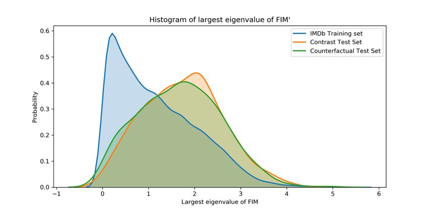
Under review as a conference paper at ICLR 2021

Figure 1: Quantifying difficulty by using the largest eigenvalue of the Fisher information metric
(FIM) a. We show that contrast sets and counterfactual examples aren’t necessarily concentrated
near the decision boundary as shown in this diagram. Difficult examples are the ones shown in green
region (close to the decision boundary) and this is the region where we should evaluate model fragility.
b. We sample points from a two-component Gaussian mixture model. We next train a classifier to
separate the two classes. c. Dataset colored by the eigenvalue of the FIM, difficult examples with a
higher eigenvalue lie closer to the decision boundary.

Mechanical Turk to create the "non-gratuitous changes." While these approaches are interesting, it’s
still unclear if evaluating on these will actually capture a classifier’s fragility. Furthermore, these
approaches significantly differ from each other and it’s important to come up with a common way to
reason about them.
Motivated by these challenges, we propose a geometrical framework to reason about difficult examples.
Using our method, we are able to discover fragile examples for state of the art NLP models like
BERTby Devlin et al. (2018) and CNN (Convolutional Neural Networks) by Kim (2014). Our
experiments using the Fisher information metric (FIM) show that both counterfactual examples and
contrast sets are, in fact, quite far from the decision boundary geometrically and not that different
from normal examples (circles and triangles in Figure 1). As such, it is more important to perform
evaluation on the examples lying in the green region, which represent confusing examples for the
classifier, where even a small perturbation (for instance, substituting the name of an actress) can
cause the neural network to misclassify. It is important to note that this does not depend solely on the
classifier’s certainty as adversarial examples can fool neural networks into misclassifying with high
confidence, as was shown by Szegedy et al. (2013).
We now motivate our choice of using the Fisher information metric (FIM) in order to quantify the
difficulty of an example. In most natural language processing tasks, deep learning models are used
to model the conditional probability distribution p(y | x) of a class label y conditioned on the input
x. Here x can represent a sentence, while y can be a sentiment of the sentence. If we imagine a
neural network as a probabilistic mapping between inputs to outputs, a natural property to measure
is the Kullback-Leibler (KL) divergence between the example and an  perturbation around that
example. For small perturbations to the input, the FIM gives a quadratic form that approximates, up
to second order, the change in the output probabilities of a neural network. Zhao et al. (2019) used
this fact to demonstrate that the eigenvector associated with the maximum eigenvalue of the FIM
gives an effective direction to perturb an example to generate an adversarial attack in computer vision.
Furthermore, from an information geometry viewpoint, the FIM is a Riemannian metric, inducing a
manifold geometry on the input space and providing a notion of distance based on changes in the
information of inputs. To the best of our knowledge, this is the first work analyzing properties of the
fisher metric to understand classifier fragility in NLP.
The rest of the paper is organized as follows: In Section 2, we summarize related work. In Section
3, we discuss our approach of computing the FIM and the gradient-based perturbation strategy. In
Section 4, we discuss the results of the eigenvalues of FIM in synthetic data and sentiment analysis
datasets with BERT and CNN. Finally, in Section 5, we discuss the implications of studying the
eigenvalues of FIM for evaluating NLP models.

                                                   2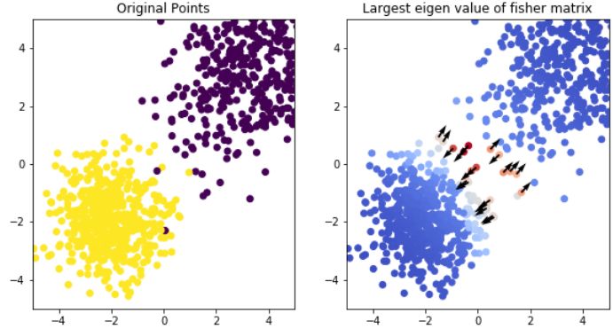
Under review as a conference paper at ICLR 2021

Table 1: CNN, IMDb dataset: Unlike the difficult examples (larger eigenvalue), word substitutions are
ineffective in changing the classifier output for the easier examples (smaller eigenvalue). In difficult
examples synonym or change of name, changes classifier label. In easy examples, despite multiple
simultaneous antonym substitutions, the classifier sentiment does not change.
 Perturbed sentiment    Word substitutions
 Positive → Negative    Going into this movie, I had heard good things about it. Coming out of it, I wasn’t really amazed nor disappointed.
 difficult    example   Simon Pegg plays a rather childish character much like his other movies. There were a couple of laughs here and there–
 (λmax =5.25)           nothing too funny. Probably my favorite → preferred parts of the movie is when he dances in the club scene. I totally
                        gotta try that out next time I find myself in a club. A couple of stars here and there including: Megan Fox, Kirsten Dunst,
                        that chick from X-Files, and Jeff Bridges. I found it quite amusing to see a cameo appearance of Thandie Newton in a
                        scene. She of course being in a previous movie with Simon Pegg, Run Fatboy Run. I see it as a toss up, you’ll either
                        enjoy it to an extent or find it a little dull. I might add, Kirsten Dunst → Nicole Kidman, Emma Stone, Megan
                        Fox, Tom Cruise, Johnny Depp, Robert Downey Jr. is adorable in this movie. :3

 Negative → Neg-        I missed this movie in the cinema but had some idea in the back of my head that it was worth a look, so when I saw
 ative easy example     it on the shelves in DVD I thought "time to watch it". Big mistake!A long list of stars cannot save this
 (λmax =0.0008)         turkey, surely one of the worst → best movies ever. An incomprehensible → comprehensible plot is poorly →
                        exceptionally delivered and poorly → brilliantly presented. Perhaps it would have made more sense if I’d read
                        Robbins’ novel but unless the film is completely different to the novel, and with Robbins assisting in the screenplay
                        I doubt it, the novel would have to be an excruciating → exciting read as well.I hope the actors were
                        well paid as they looked embarrassed to be in this waste of celluloid and more lately DVD blanks, take for example Pat
                        Morita. Even Thurman has the grace to look uncomfortable at times.Save yourself around 98 minutes of
                        your life for something more worthwhile, like trimming your toenails or sorting out your sock drawer. Even when you
                        see it in the "under $5" throw-away bin at your local store, resist the urge!

2    R ELATED W ORK

In NLP, machine learning models for classification rely on spurious statistical patterns of the text
and use shortcut for learning to classify. These can range from annotation artifacts, as was shown
by Goyal et al. (2017); Kaushik and Lipton (2018); Gururangan et al. (2018), spelling mistakes as
in McCoy et al. (2019), or new test conditions that require world knowledge Glockner et al. (2018).
Simple decision rules that the model relies on are hard to quantify. Trivial patterns like relying on
the answer “2” for answering questions of the format “how many” for the visual question answering
dataset Antol et al. (2015), would correctly answer 39% of the questions. Jia and Liang (2017)
showed that adversarially inserted sentences that did not change the correct answer, would cause
state of the art models to regress in performance in the SQuAD Rajpurkar et al. (2016) question
answering dataset. Glockner et al. (2018) showed that template-based modifications by swapping
just one word from the training set to create a test set highlighted models’ failure to capture many
simple inferences. Dixon et al. (2018) evaluated text classifiers using a synthetic test set to understand
unintended biases and statistical patterns. Using a standard set of demographic identity terms, the
authors reduce the unintended bias without hurting the model performance. Shen et al. showed that
word substitution strategies include stylistic variations that change the sentiment analysis algorithms
for similar word pairs. Evaluations of these models through perturbations of the input sentence are
crucial to evaluating the robustness of models.
Another issue of language recently has been that static benchmarks like GLUE by Wang et al. (2018)
tend to saturate quickly because of the availability of ever-increasing compute and harder benchmarks
are needed like SuperGlue by Wang et al. (2019). A more sustainable approach to this is the
development of moving benchmarks, and one notable initiative in this area is the Adversarial NLI by
Nie et al. (2019), but most of the research community hardly validate their approach against this sort
of moving benchmark. In the Adversarial NLI dataset, the authors propose an iterative, adversarial
human-and-model-in-the-loop solution for Natural Language Understanding dataset collection, where
the goal post continuously shifts about useful benchmarks and makes models robust by training the
model iteratively on difficult examples. Approaches like never-ending learning byMitchell et al.
(2018) where models improve, and test sets get difficult over time is critical. A moving benchmark is
necessary since we know that improving performance on a constant test set may not generalize to
newly collected datasets under the same condition Recht et al. (2019); Beery et al. (2018). Therefore,
it is essential to find difficult examples in a more disciplined way.
Approaches based on geometry have recently started gaining traction in computer vision literature.
Zhao et al. (2019) et al used a similar approach for understanding adversarial examples in images.

                                                                            3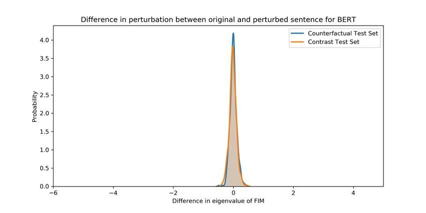
Under review as a conference paper at ICLR 2021

3    M ETHODS

A neural network with discrete output can be thought of as a mapping between a manifold of
inputs to the discrete output space. Most traditional formulations treat this input space as flat, thus
reasoning that the gradient of the likelihood in input space gives us the direction which causes the
most significant change in terms of likelihood. However, by imagining the input as a pullback of
the output, we obtain a non-linear manifold where the euclidean metric no longer suffices. A more
appropriate choice thus is to use the fisher information as a Riemannian metric tensor.
We first introduce the Fisher Metric formulation for language. For the purposes of the derivation
below the following notations are used.

x : Vector of input sentence. This is an n * d sentence where n is the number of words in
the sentence and d is the dimensionality of the word embedding.
y : Label of class, in our context that is the positive or the negative sentiment.
p(y|x) : The conditional probability distribution between y and x.
KL(p, q) : The KL divergence between distributions p and q for two sentences
∇f (x) : Gradient of a function of f w.r.t x
∇2 f (x) : Hessian of f(x) w.r.t x
We apply the a perturbation η to modifying a sentence to create a new sentence (eg., a counterfactual
example). We can then see the effect of this perturbation η in terms of change in the probability
distribution over labels. Ideally, we would like to find points where a small perturbation can result in
a large change in the probability distribution over labels.

              KL(p(y|x)||p(y|x + η)) = −Ep(y|x) logp(y|x) + Ep(y|x) logp(y|x + η)

We now perform a Taylor expansion of the first term on the right hand side

       = −Ep(y|x) (logp(y|x) + η∇logp(y|x) + η T ∇2 logp(y|x)η + ...) + Ep(y|x) logp(y|x)

                                    ∼ −Ep(y|x) η T ∇2 logp(y|x)η

Since the expectation of score is zero and the first and last terms cancel out, we are left with.

                                               = η T Gη

Where G is the FIM. By studying the eigenvalues of this matrix locally, we can quantify if small
change in η can cause a large change in the distribution over labels. We use the largest eigenvalue
of the FIM as a score to quantify the “difficulty” of an example. We now propose the following
algorithm to compute the FIM:
After getting the eigenvalues of the FIM, we can use the largest eigenvalue λmax to quantify
how fragile an example is to linguistic perturbation. At points with largest eigenvalues, smaller
perturbations can be much more effective in changing the classifier output. These examples, thus, are
also more confusing and more difficult for the model to classify.

                                                   4
Under review as a conference paper at ICLR 2021
Table 2: CNN, Counterfactual Examples: In difficult examples (larger eigenvalue), individual
synonym/antonym substitutions are effective in changing the classifier output. In easy examples
(smaller eigenvalue) multiple antonym substitutions simultaneously have no effect on the classifier
output.
Perturbed sentiment Word substitutions
Positive → Negative This move was on TV last night. I guess as a time filler, because it was incredible! The movie is just an entertainment
difficult example piece to show some talent at the start and throughout. (Not bad talent at all). But the story is too brilliant for words.
λmax =4.38 The "wolf", if that is what you can call it, is hardly shown fully save his teeth. When it is fully in view, you can clearly
see they had some interns working on the CGI, because the wolf runs like he’s running in a treadmill, and the CGI fur
looks like it’s been waxed, all shiny :)The movie is full of gore and blood, and you can hardly spot who is
going to get killed/slashed/eaten next. Even if you like these kind of splatter movies you will be surprised, they did do
a good job at it.Don’t even get me started on the actors... Very amazing lines and the girls hardly scream
at anything. But then again, if someone asked me to do good acting just to give me a few bucks, then hey, where do I
sign up?Overall exciting → boring, extraordinary, uninteresting, exceptional and frightening horror.
Negative → Neg- I couldn’t stand this movie. It is a definite waste of a movie. It fills you with boredom. This movie is not worth the
ative easy example rental or worth buying. It should be in everyones trash. Worst → Excellent movie I have seen in a long time. It will
λmax =0.013 make you mad because everyone is so mean to Carl Brashear, but in the end it gets only worse. It is a story of cheesy
romance, bad → good drama, action, and plenty of unfunny → funny lines to keep you rolling your eyes. I hated
a lot of the quotes. I use them all the time in mocking the film. They did not help keep me on task of what I want to do.
It shows that anyone can achieve their dreams, all they have to do is whine about it until they get their way. It is a long
movie, but every time I watch it, I dradr that it is as long as it is. I get so bored in it, that it goes so slow. I hated this
movie. I never want to watch it again.
Algorithm 1 Algorithm for estimating difficulty of an example
Input: x, f
Output: λmax
Calculate probability vector :
1: p = f (x)
Calculate Jacobian of log probability w.r.t x
2: J = ∇x logp
Duplicate probability vector along rows to match J’s shape
3: pc = duplicate(p, J.dim[0])
Compute the FIM
4: G = pc JJ T
Perform eigendecomposition to get the eigenvalues
5: λs , vs = eigendecomposition(G)
6: return max(λs )
3.1 G RADIENT ATTRIBUTION BASED P ERTURBATION
In our perturbations, we rely on Integrated Gradients (IG) by Sundararajan et al. (2017), since IG
satisfies both sensitivity (network gradients to focus on relevant input feature attributes of the model
with respect to the output) and implementation invariance of the neural network. IG allows us to
assign relative importance to each word token in the input. After computing the token attributions
with IG, we only perturb those words for “easy” and “difficult” examples. Once we compute
the feature attribution for each input word in the sentence, we find the most important words by
thresholding the attribution score. We then test the classifier’s fragility by substituting these words
for their synonyms/antonyms, etc, and checking if the classifier prediction changes. We show that
easy examples are robust to significant edits with multiple positive tokens like “excellent”, “great”
substituted simultaneously, and “difficult” examples change predictions from positive to negative
with meaningless substitutions like names of actors and actresses.
4 D ISCUSSION AND R ESULTS
4.1 FIM REFLECTS DISTANCES FROM THE DECISION BOUNDARY
We first investigate the FIM properties by training a neural network on a synthetic mixture of gaussians
dataset. The parameters of the two gaussians are µ1 = [−2, −2] and µ2 = [3.5, 3.5]. The covariances
are Σ1 = eye(2) and Σ2 = [[2., 1.], [1., 2.]] The dataset is shown in figure 1. We train a 2-layered
network to separate the two classes from each other. We use algorithm 1 to compute the largest
5Under review as a conference paper at ICLR 2021
eigenvalue of the FIM for each datapoint and use it to color the points. We also plot the eigenvector
for the top 20 points.
As seen by the gradient of the colors in Figure 1, the points with the largest eigenvalue of the FIM
lie close to the decision boundary. These points are indicative of how confusing the example is to
the neural network since a small shift along the eigenvector can cause a significant change in the KL
divergence between the probability distribution of the original and new data points. These points
with a high eigenvalue are close to the decision boundary, and these examples are most susceptible to
perturbations.
4.2 FIM VALUES CAPTURE RESILIENCE TO LINGUISTIC PERTURBATIONS , Q UALITATIVE
E XPLORATION
4.2.1 CNN
For the difficult examples, we tried the following trivial substitutions one at a time: a) a synonym b) a
semantically equivalent word c) an antonym d) substituting the name of an actress present in the same
passage. As seen in Table 1, either replacing favorite with preferred or “Kirsten Dunst” with any
of the listed actors/actresses suffices to change the classifier’s prediction. Note that, “Megan Fox’s”
name appears in the same review in the previous sentence. Similar in Table 3, for counterfactual
examples, it’s sufficient to replace “exciting” with either an antonym (“boring” or “uninteresting”) or
a synonym (“extraordinary” or “exceptional”). We see the same pattern in contrast sets in Appendix.
For easy examples however, despite trying to replace four or more high attribution words simultane-
ously with antonyms, the predicted sentiment did not change. Substitutions include “good” to “bad”,
“unfunny” to “funny”, “factually correct” to “factually incorrect”. Even though the passage included
words like “boredom”, a word that is generally associated with a negative movie review, the model
did not assign it a high attribution score. Consequently, we did not try to substitute these words for
testing robustness or fragility of word substitutions.
Figure 2: Left figure: The difficult examples on the FIM test set are challenging for the classifiers with
accuracy between 1-5%. For the easy examples, (low FIM λmax ) the accuracy ranges between 60-
100%. Right figure: We plot the classifier accuracy with respect to the l2 norm of the perturbation in
embedding space. For difficult examples, the classifier accuracy drops below 5% at small perturbation
strengths (l2 norm < 0.3)
4.2.2 BERT
BERT: Transfer learned models like BERT capture rich semantic structure of the sentence. They are
robust to changes like actor names and tend to rely on semantically relevant words for classifying
movie reviews. As we can see from Table 6 difficult BERT examples, even with multiple positive
words, tend to predict a negative sentiment when only one of the positive word is substituted. Even
with words like “fantastic”, “terrific” and “exhilarating”, just changing “best” to “worst” changed
the entire sentiment of the movie review. Easy examples for BERT require multiple simultaneous
word substitutions to change the sentiment as can be seen in Table 6. Unlike CNN models, BERT is
significantly more robust to meaningless substitutions like actor names.
6Under review as a conference paper at ICLR 2021
Figure 3: On YelpReviewPolarity we observe a correlation coefficient of -0.4 between minimum
perturbation strength and the difficulty score. Similarly, we observe a correlation of 0.35 between the
difficulty score and empirical success of random word substitutions. This suggests that fim eigenvalue
captures perturbation sensitivity in both embedding space and word substitutions.
Figure 4: a) Distribution of difference in largest eigenvalue of FIM of the original and the perturbed
sentence in contrast set and counterfactual examples for BERT and CNN. With a mean near 0, these
perturbations are not difficult for the model. Adhoc perturbations are thus not useful for evaluating
model robustness.
4.3 H IGH FIM EXAMPLES ARE CHALLENGING TO NLP CLASSIFIERS , Q UANTITATIVE
E XPERIMENTS
4.3.1 BAG OF T RICKS FOR EFFICIENT TEXT CLASSIFICATION
When the dataset size is increased, simple models perform competitively to models like BERT
Wang et al. (2020). We use the bag of tricks for efficient text classification Joulin et al. (2017)
for its inference and training speed and strong performance on text classification on 5 popular text
classification datasets (YelpReviewPolarity, AGNEWS, SogouNews, YelpReviewFull and Yahoo
Answers)
In order to investigate the relationship between classifier performance and FIM eigenvalues we
select n-smallest and n-largest fim examples from the test set. We randomly chose a perturbation
strength between 0 and 1 and we perturb the example along the largest eigenvector proportional to
the chosen perturbation strength. As can be seen from figure 2 left, despite sampling a large range
of difficult examples, between (125-1200), the classifier performed poorly on the difficult set with
the accuracy failing to exceed 9%. On the easy set however, the classifier accuracy never falls below
7Under review as a conference paper at ICLR 2021
57.5%. In figure 2b, we plot the classifier accuracy as a function of perturbation strength (l2 norm of
perturbation vector for difficult examples, even small perturbations upto 0.4 l2 norm, cause a 17%
reduction in accuracy. For easy examples however even upto a l2 norm of 1 barely result in any drop
in performance. More examples are in Appendix A.
We randomly sample 500 examples and perturb the examples along the largest eigenvector. We use
binary search to determine the minimum perturbation strength sufficient to flip the classifier output.
As we can see from Figure 3, a correlation of -0.4 implies it is possible to misclassify larger FIM
examples by applying a small perturbation strength. In order to investigate the relationship between
FIM and random word substitutions, we flipped 10% of the words in a document, for 500 randomly
sampled examples. As seen in Figure 3b, a correlation of 0.35 implies that difficult examples, (larger
FIM eigenvalues) are more susceptible to random word substitutions.
4.4 D O CONTRAST SETS AND COUNTERFACTUAL EXAMPLES LIE CLOSE TO THE DECISION
BOUNDARY ?
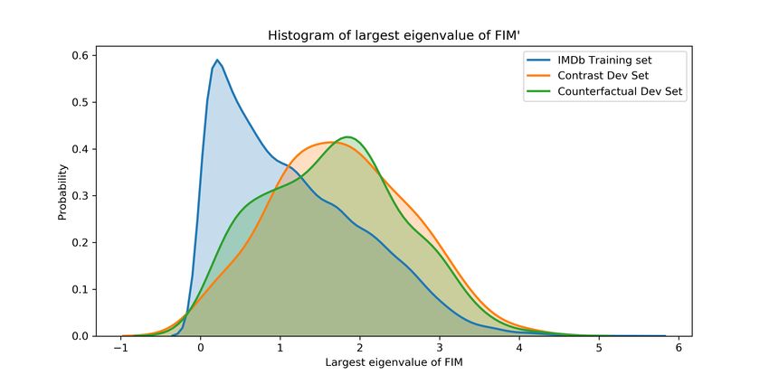
We first plot the distribution of eigenvalues of IMDb examples, counterfactual examples and contrast
sets examples in Figure 2. If the goal is to evaluate examples near the decision boundary the contrast
set/counterfactual eigenvalue distribution should be shifted to the right with very little overlap with
the original examples. However, as we can see from Figure 2, we see a 69.38% overlap between
contrast sets and IMDb examples as well as a 73.58% overlap between counterfactual and IMDb
examples for the CNN model that was only trained on IMDb training set. The presence of significant
overlap between the three distributions indicate that counterfactual/contrast examples are not more
difficult for the model compared to the normal examples. Furthermore, since the FIM capture distance
from the decision boundary, most counterfactual and contrast sets lie as far away from the decision
boundary as the original IMDb dataset examples.
We next quantify the effect of changing the original sentence to the perturbed sentence in counter-
factual/contrast test sets. We plot the distribution of difference in eigenvalue of the original and
perturbed sentence in Figure 2. 30% of the counterfactual examples (area to the right of 0) did not
increase the FIM eigenvalue and the perturbation was ineffective. For contrast sets, this number is
around 70% (area to the right of 0), hinting that majority of perturbations are not useful for testing
model robustness. A subtle point to note here, even though 70% of counterfactual examples increase
the difficulty, it’s because we have chosen a weak threshold (0) to quantify the usefulness of the
perturbation. A more practical threshold like 1 would lead to lesser number of useful examples for
both counterfactual and contrast set examples.
5 I MPLICATIONS
5.1 C ONSTRUCTING T EST SET BY PERTURBING HIGH FIM EXAMPLES
As evident from figure 2, high FIM examples are particularly challenging for NLP classifiers. This
makes them useful to understand model performance. By sampling the high FIM examples and
perturbing them slightly in embedding space, we can construct a new test set to evaluate NLP models.
By repeating this process multiple times, more robust classifiers can be created.
5.2 NLP MODELS SHOULD BE EVALUATED AT THE EXAMPLES NEAR THE DECISION
BOUNDARY
Deep learning models because of their high representation capacity are good at memorizing the
training set. In the absence of sufficient variation in the test set, this can lead to an inflation in
accuracy without actual generalization. However, examples near the decision boundary of a classifier,
show the fragilities of these classifiers. These are the examples that are most susceptible to shallow
feature learning and thus are the ones that need to be tested for fragility and word substitutions. Our
approach based on FIM score, provides a task and architecture agnostic approach to discovering such
examples.
8Under review as a conference paper at ICLR 2021
Table 3: Statistics of difference in largest FIM eigenvalue (pre and post perturbation) for counterfactual
examples and contrast sets.
Architecture Dataset Type Mean Std
CNN Counterfactual Examples Dev -0.55 1.17
Test -0.57 1.22
CNN Contrast Sets Dev 0.56 0.89
Test 0.65 1.15
BERT Counterfactual Examples Dev 0.004 0.10
Test 0.003 0.11
BERT Contrast Sets Dev 0.02 0.10
Test -0.01 0.11
5.3 I NVESTIGATE HIGH FIM EXAMPLES WITH I NTEGRATED G RADIENTS TO UNDERSTAND
MODEL FRAGILITY
For our models, difficult examples have a mix of positive and negative words in a movie review. The
models also struggled with examples of movies that selectively praise some attributes like acting
(e.g., "Exceptional performance of the actors got me hooked to the movie from the beginning") while
simultaneously use negative phrases (e.g., "however the editing was horrible"). Difficult examples
also have high token attributions associated with irrelevant words like "nuclear," "get," and "an."
Thus substituting one or two words in difficult examples change the predicted label of the classifier.
Similarly, easier examples have clearly positive reviews (e.g., "Excellent direction, clever plot and
gripping story"). Combining integrated gradients with high FIM examples can thus yield insights
into the fragility of NLP models.
5.4 P ERTURBATION SHOULD BE PERFORMED ALONG THE LARGEST EIGENVECTOR
The eigenvector corresponding to λmax represents the direction of largest change in probability
distribution over output. This makes it a useful candidate direction to evaluate model fragility while
random word substitutions are easier to interpret, they might end up being orthogonal to the largest
eigenvector and thus not capture model fragility effectively. One strategy to circumvent this issue is
to find word substitutions with a large projection on this eigenvector.
6 C ONCLUSION
We have proposed a geometrical method to quantify the difficulty of an example in NLP. Our method
identified fragilities in state of the art NLP models like BERT and CNN. By directly modeling the
impact of perturbation in natural language through the Fisher information metric, we showed that
examples close to the decision boundary are sensitive to meaningless changes. We also showed
that counterfactual examples and contrast sets don’t necessarily lie close to the decision boundary.
Furthermore, depending on the distance from the decision boundary, small innocuous tweaks to a
sentence might actually correspond to a large change in the embedding space. Thus one has to be
careful in constructing perturbations, and more disciplined approaches are needed to address the
same.
As our methods are agnostic to the choice of architecture or dataset, in future we plan to extend
this to other NLP tasks and datasets. We are also studying the properties of the decision boundary:
whether different classifiers have a similar decision boundary, are there universal difficult examples
which confound multiple classifiers? We also plan to investigate strategies for automatic generation
of sentence perturbations based on the largest eigenvector of the FIM. Even though we have explored
difficult examples from a classifier’s perspective, we are also interested in exploring the connections
between FIM and perceived difficulty of examples by humans.
R EFERENCES
Stanislaw Antol, Aishwarya Agrawal, Jiasen Lu, Margaret Mitchell, Dhruv Batra, C Lawrence Zitnick,
and Devi Parikh. Vqa: Visual question answering. In Proceedings of the IEEE international
9Under review as a conference paper at ICLR 2021
conference on computer vision, pages 2425–2433, 2015.
Sara Beery, Grant Van Horn, and Pietro Perona. Recognition in Terra Incognita. pages 456–
473, 2018. URL http://openaccess.thecvf.com/content_ECCV_2018/html/
Beery_Recognition_in_Terra_ECCV_2018_paper.html.
Jacob Devlin, Ming-Wei Chang, Kenton Lee, and Kristina Toutanova. Bert: Pre-training of deep
bidirectional transformers for language understanding. arXiv preprint arXiv:1810.04805, 2018.
Lucas Dixon, John Li, Jeffrey Sorensen, Nithum Thain, and Lucy Vasserman. Measuring and
mitigating unintended bias in text classification. In Proceedings of the 2018 AAAI/ACM Conference
on AI, Ethics, and Society, pages 67–73, 2018.
Matt Gardner, Yoav Artzi, Victoria Basmova, Jonathan Berant, Ben Bogin, Sihao Chen, Pradeep
Dasigi, Dheeru Dua, Yanai Elazar, Ananth Gottumukkala, Nitish Gupta, Hanna Hajishirzi, Gabriel
Ilharco, Daniel Khashabi, Kevin Lin, Jiangming Liu, Nelson F. Liu, Phoebe Mulcaire, Qiang Ning,
Sameer Singh, Noah A. Smith, Sanjay Subramanian, Reut Tsarfaty, Eric Wallace, Ally Zhang, and
Ben Zhou. Evaluating NLP Models via Contrast Sets. arXiv:2004.02709 [cs], April 2020. URL
http://arxiv.org/abs/2004.02709. arXiv: 2004.02709.
Robert Geirhos, Jörn-Henrik Jacobsen, Claudio Michaelis, Richard Zemel, Wieland Brendel, Matthias
Bethge, and Felix A. Wichmann. Shortcut Learning in Deep Neural Networks. arXiv:2004.07780
[cs, q-bio], April 2020. URL http://arxiv.org/abs/2004.07780. arXiv: 2004.07780.
Max Glockner, Vered Shwartz, and Yoav Goldberg. Breaking nli systems with sentences that require
simple lexical inferences. arXiv preprint arXiv:1805.02266, 2018.
Yash Goyal, Tejas Khot, Douglas Summers-Stay, Dhruv Batra, and Devi Parikh. Making the v in vqa
matter: Elevating the role of image understanding in visual question answering. In Proceedings of
the IEEE Conference on Computer Vision and Pattern Recognition, pages 6904–6913, 2017.
Suchin Gururangan, Swabha Swayamdipta, Omer Levy, Roy Schwartz, Samuel R. Bowman, and
Noah A. Smith. Annotation Artifacts in Natural Language Inference Data. arXiv:1803.02324 [cs],
April 2018. URL http://arxiv.org/abs/1803.02324. arXiv: 1803.02324.
Robin Jia and Percy Liang. Adversarial examples for evaluating reading comprehension systems.
arXiv preprint arXiv:1707.07328, 2017.
Armand Joulin, E. Grave, P. Bojanowski, and Tomas Mikolov. Bag of tricks for efficient text
classification. ArXiv, abs/1607.01759, 2017.
Divyansh Kaushik and Zachary C Lipton. How much reading does reading comprehension require?
a critical investigation of popular benchmarks. arXiv preprint arXiv:1808.04926, 2018.
Divyansh Kaushik, Eduard Hovy, and Zachary C. Lipton. Learning the Difference that Makes a
Difference with Counterfactually-Augmented Data. arXiv:1909.12434 [cs, stat], February 2020.
URL http://arxiv.org/abs/1909.12434. arXiv: 1909.12434.
Yoon Kim. Convolutional neural networks for sentence classification. arXiv preprint arXiv:1408.5882,
2014.
R Thomas McCoy, Ellie Pavlick, and Tal Linzen. Right for the wrong reasons: Diagnosing syntactic
heuristics in natural language inference. arXiv preprint arXiv:1902.01007, 2019.
Tom Mitchell, William Cohen, Estevam Hruschka, Partha Talukdar, Bishan Yang, Justin Betteridge,
Andrew Carlson, Bhanava Dalvi, Matt Gardner, Bryan Kisiel, et al. Never-ending learning.
Communications of the ACM, 61(5):103–115, 2018.
Yixin Nie, Adina Williams, Emily Dinan, Mohit Bansal, Jason Weston, and Douwe Kiela. Adversarial
nli: A new benchmark for natural language understanding. arXiv preprint arXiv:1910.14599, 2019.
10Under review as a conference paper at ICLR 2021
Adam Poliak, Jason Naradowsky, Aparajita Haldar, Rachel Rudinger, and Benjamin Van Durme.
Hypothesis Only Baselines in Natural Language Inference. In Proceedings of the Seventh Joint
Conference on Lexical and Computational Semantics, pages 180–191, New Orleans, Louisiana,
June 2018. Association for Computational Linguistics. doi: 10.18653/v1/S18-2023. URL https:
//www.aclweb.org/anthology/S18-2023.
Pranav Rajpurkar, Jian Zhang, Konstantin Lopyrev, and Percy Liang. Squad: 100,000+ questions for
machine comprehension of text. arXiv preprint arXiv:1606.05250, 2016.
Benjamin Recht, Rebecca Roelofs, Ludwig Schmidt, and Vaishaal Shankar. Do imagenet classifiers
generalize to imagenet? arXiv preprint arXiv:1902.10811, 2019.
Judy Hanwen Shen, Lauren Fratamico, Iyad Rahwan, and Alexander M Rush. Darling or babygirl?
investigating stylistic bias in sentiment analysis.
Mukund Sundararajan, Ankur Taly, and Qiqi Yan. Axiomatic attribution for deep networks. In
Proceedings of the 34th International Conference on Machine Learning-Volume 70, pages 3319–
3328. JMLR. org, 2017.
Christian Szegedy, Wojciech Zaremba, Ilya Sutskever, Joan Bruna, Dumitru Erhan, Ian Goodfellow,
and Rob Fergus. Intriguing properties of neural networks. arXiv preprint arXiv:1312.6199, 2013.
Alex Wang, Amanpreet Singh, Julian Michael, Felix Hill, Omer Levy, and Samuel R Bowman. Glue:
A multi-task benchmark and analysis platform for natural language understanding. arXiv preprint
arXiv:1804.07461, 2018.
Alex Wang, Yada Pruksachatkun, Nikita Nangia, Amanpreet Singh, Julian Michael, Felix Hill, Omer
Levy, and Samuel Bowman. Superglue: A stickier benchmark for general-purpose language
understanding systems. In Advances in Neural Information Processing Systems, pages 3261–3275,
2019.
Sinong Wang, Madian Khabsa, and Hao Ma. To pretrain or not to pretrain: Examining the benefits of
pretrainng on resource rich tasks. In Proceedings of the 58th Annual Meeting of the Association
for Computational Linguistics, pages 2209–2213, 2020.
Thomas Wolf, Lysandre Debut, Victor Sanh, Julien Chaumond, Clement Delangue, Anthony Moi,
Pierric Cistac, Tim Rault, Rémi Louf, Morgan Funtowicz, Joe Davison, Sam Shleifer, Patrick von
Platen, Clara Ma, Yacine Jernite, Julien Plu, Canwen Xu, Teven Le Scao, Sylvain Gugger, Mariama
Drame, Quentin Lhoest, and Alexander M. Rush. Huggingface’s transformers: State-of-the-art
natural language processing. ArXiv, abs/1910.03771, 2019.
Chenxiao Zhao, P Thomas Fletcher, Mixue Yu, Yaxin Peng, Guixu Zhang, and Chaomin Shen. The
adversarial attack and detection under the fisher information metric. In Proceedings of the AAAI
Conference on Artificial Intelligence, volume 33, pages 5869–5876, 2019.
11Under review as a conference paper at ICLR 2021
A PPENDIX A
CNN and BERT:
We train a convolutional neural network (CNN) with a 50d GloVe embedding on the IMDb dataset,
and calculate the eigenvalue of the FIM for each example. The accuracy on the IMDb test set
was around 85.4%. For all experiments in the paper the model was trained on the original 25000
examples in the original IMDb training split with a 90% train and 10% valid split. For all experiments
in the paper, we did not train on the counterfactual or contrast set examples to fairly evaluate the
robustness to perturbations of contrast sets and counterfactual examples. For BERT we finetuned
’bert-base-uncased’ and achieved an accuracy of 92.6% using huggingface transformers by Wolf
et al. (2019). We evaluated the largest eigenvalue of the dev and test sets of the contrast set and
counterfactual examples datasets of IMDb.
Bag of Tricks for efficient text classification:
We use unigram and bigram word embeddings. The latent dimension is 32. We use torchtext datasets
directly available for the training and test splits. We use the SGD optimizer with a learning rate of 4
and train each model for 8 epochs. We use a learning rate scheduler with a gamma of 0.9.
12Under review as a conference paper at ICLR 2021
A PPENDIX B
13Under review as a conference paper at ICLR 2021
Figure 5: Here we take the Joulin et al. (2017) text classification approach ( and plot classifier
accuracy as a function of the step size of the perturbation. The number of examples in the x-axis
represents the number of examples based on the eigenvalue. So, 200 refers to the 200 easy examples
and 200 difficult examples. We then perturb these examples in the direction of the eigenvector and
check if the classifier prediction flipped. As can be seen that the classifier accuracy remains very high
for easy examples and is significantly low for difficult examples. On the second diagram, for easy
examples, the classifier still exhibits minimal performance drop when the weight of the perturbation
along the eigenvector is increased. Thus our method is dataset agnostic.
Figure 6: We use the eigenvector with the largest eigenvalue as a perturbation in embedding space.
As we can see there is a linear relationship between log lambda max and the perturbation strength
needed to flip the classifier output. We use binary search between the range (0,6) to discover the
minimal l2 norm perturbation along the largest eigenvector which can successfully flip the classifier’s
output. For each dataset, we select 500 random examples from the test set for the perturbation. Note
the negative slope in all the datasets. The p-value and the r-value are reported at the top. The log of
the largest fim eigenvalue is on the x-axis. Thus, an example with a small eigenvalue requires a larger
perturbation to flip classifier prediction than an example with large fim eigenvalue.
14Under review as a conference paper at ICLR 2021
Figure 7: We notice the linear relationship between the log of eigenvalue and the percentage of
successful word flips. Since the length of each document varies drastically for these document
classification problems, we decide the number of words to flip as 10% of the document length with
the vocabulary of the dataset. We then measure the percentage of predictions whose classification
label changes and the log of fim eigenvalue. The pv alue and the rv alue are reported at the top.
A PPENDIX C
Figure 8: a) Histogram of eigenvalues of dev sets of original IMDb examples, contrast sets and
counterfactual examples. The significant overlap between the three distributions indicates that the
counterfactual and contrast set examples might not be as difficult as previously believed. The tail
end of all three distributions contain the difficult examples. b) Distribution of difference in largest
eigenvalue of FIM of the original and the perturbed sentence in contrast set and counterfactual
examples. With a mean near 0, these perturbations are not necessarily more difficult for the model.
15Under review as a conference paper at ICLR 2021
Table 4: Perturbing an easy example on the IMDb dataset: The first row represents original sentence.
As we can see here, most perturbations are ineffective in changing the FIM eigenvalue and thus the
difficulty of the example. Despite multiple substitutions (last row), we are only able to achieve a
modest increase in FIM score, indicating the resilience to perturbations.
Perturbed sen- Word substitutions
timent
Negative → Probably the worst Dolph film ever. There’s nothing you’d want or expect here. Don’t waste
Negative your time. Dolph plays a miserable cop with no interests in life. His brother gets killed and
easy example Dolph tries to figure things out. The character is just plain stupid and stumbles around aimlessly.
(λmax =0.0007) Pointless.
Negative → Probably the worst Dolph film ever. There’s nothing → everything you’d want or expect here.
Negative mi- Don’t waste your time. Dolph plays a miserable cop with no interests in life. His brother gets
nor change killed and Dolph tries to figure things out. The character is just plain stupid and stumbles around
in FIM value aimlessly. Pointless.
(λmax =0.0008)
Negative → Probably the worst Dolph film ever. There’s nothing you’d want or expect here. Don’t waste
Negative mi- your time. Dolph plays → portrays a miserable cop with no interests in life. His brother gets
nor change killed and Dolph tries to figure things out. The character is just plain stupid and stumbles around
in FIM value aimlessly. Pointless.
(λmax =0.0005)
Negative → Probably the worst Dolph film ever. There’s nothing you’d want or expect here. Don’t waste
Negative mi- your time. Dolph plays → portrays a miserable cop with no interests in life. His brother gets
nor change killed and Dolph tries → attempts to figure things out. The character is just plain stupid and
in FIM value stumbles around aimlessly. Pointless.
(λmax =0.0007)
Negative → Probably the best Dolph film ever. There’s everything you’d want or expect here. Spend your
Negative time. Dolph portrays a miserable cop with lots of interests in life. His brother gets killed and
Significant in- Dolph attempts to figure things out. The character is just plain amazing.
crease in FIM
(λmax =1.56)
16Under review as a conference paper at ICLR 2021
Table 5: Perturbing a difficult example on the IMDb dataset: The first row represents original
sentence. Unlike easy examples, difficult examples tend to have a mixture of positive and negative
traits. Furthermore, a minor perturbation like removal of a sentence (row 1) or substitution of a word
(row 2) causes a significant drop in FIM eigenvalue. The small FIM score indicates that the perturbed
review is not difficult for the classifier.
Perturbed sen- Word substitutions
timent
Negative → It really impresses me that it got made. The director/writer/actor must be really charismatic
Negative diffi- in reality. I can think of no other way itd pass script stage. What I want you to consider is
cult example this...while watching the films I was feeling sorry for the actors. It felt like being in a stand up
(λmax =5.47) comedy club where the guy is dying on his feet and your sitting there, not enjoying it, just feeling
really bad for him coz hes of trying. Id really like to know what the budget is, guess it must have
been low as the film quality is really poor. I want to write ’the jokes didn’t appeal to me’. but the
reality is for them to appeal to you, you’d have to be the man who wrote them. or a retard. So
imagine that in script form...and this guy got THAT green lit. Thats impressive isn’t it?
Negative → It really impresses me that it got made. The director/writer/actor must be really charismatic
Negative in reality. I can think of no other way itd pass script stage. What I want you to consider is
Significant this...while watching the films I was feeling sorry for the actors. It felt like being in a stand up
change in FIM comedy club where the guy is dying on his feet and your sitting there, not enjoying it, just feeling
(λmax =0.640) really bad for him coz hes of trying. Id really like to know what the budget is, guess it must have
been low as the film quality is really poor. I want to write ’the jokes didn’t appeal to me’. but the
reality is for them to appeal to you, you’d have to be the man who wrote them. or a retard. So
imagine that in script form...and this guy got THAT green lit. Thats impressive isn’t it?
Negative → It really impresses me that it got made. The director/writer/actor must be really charismatic
Negative in reality. I can think of no other way itd pass script stage. What I want you to consider is
Significant this...while watching the films I was feeling sorry for the actors. It felt like being in a stand up
change in FIM comedy club where the guy is dying on his feet and your sitting there, not enjoying it, just feeling
(λmax =0.445) really bad for him coz hes of trying. Id really like to know what the budget is, guess it must have
been low as the film quality is really poor. I want to write ’the jokes didn’t appeal to me’. but the
reality is for them to appeal to you, you’d have to be the man who wrote them. or a retard. So
imagine that in script form...and this guy got THAT green lit. Thats impressive → weird isn’t
it?
Table 6: BERT: Difficult Examples change sentiment with a single word substituted. Easy examples,
however, retain positive sentiment despite multiple substitutions of positive words with negative
words.
Perturbed sentiment Word substitutions
Positive → Negative OK, I kinda like the idea of this movie. I’m in the age demographic, and I kinda identify with some of the stories. Even
difficult example the sometimes tacky and meaningful dialogue seems realistic, and in a different movie would have been forgivable.I’m trying as hard as possible not to trash this movie like the others did, but it’s easy when the filmmakers were
trying very hard.The editing in this movie is terrific! Possibly the best → worst editing I’ve ever seen
in a movie! There are things that you don’t have to go to film school to learn, leaning good editing is not one of them,
but identifying a bad one is.Also, the shot... Oh my God the shots, just fantastic! I can’t even go into the
details, but we sometimes just see random things popping up, and that, in conjunction with the editing will give you
the most exhilirating film viewing experience.This movie being made on low or no budget with 4 cast and
crew is an excuse also. I’ve seen short films on youtube with a lot less artistic integrity! ...
Positive → Posi- This is the best and most original show seen in years. The more I watch it the more I fall in love with → hate it. The
tive easy example cast is excellent → terrible , the writing is great → bad. I personally loved → hated every character. However,
(λmax =0.55) there is a character for everyone as there is a good mix of personalities and backgrounds just like in real life. I believe
ABC has done a great service to the writers, actors and to the potential audience of this show, to cancel so quickly and
not advertise it enough nor give it a real chance to gain a following. There are so few shows I watch anymore as most
TV is awful . This show in my opinion was right down there with my favorites Greys Anatomy and Brothers and Sisters.
In fact I think the same audience for Brothers and Sisters would hate this show if they even knew about it.
17Under review as a conference paper at ICLR 2021
Table 7: Counterfactual perturbations cause reduction in difficulty: The original example is more
difficult than the perturbed counterfactual example because of strong giveaway words like "amazing".
The subtle changes to make the sentence positive like changing the amount or the rating almost makes
no difference. Instead, the use of a strong word “amazing” makes the sentence extremely easy for the
model to classify as positive. The heavy reliance on a single word for the positive example makes
this much easier to classify than the original sentence which used the word “odd” (a word that is not
necessarily negative) as a negative sentiment.
Perturbed sen- Word substitutions
timent
Negative → Definitely an odd debut for Michael Madsen. Madsen plays Cecil Moe, an alcoholic family
Negative diffi- man whose life is crumbling all around him. Cecil grabs a phone book, looks up the name of a
cult example preacher, and calls him in the middle of the night. He goes to the preacher’s home and discusses
(λmax =3.42) his problems. The preacher teaches Cecil to respect the word of God and have Jesus in his heart.
That makes everything all better. Ahh...if only everything in life were that easy. The fact that this
"film" looks as if it was made with about $500 certainly doesn’t help. 1/10
Positive → Definitely an amazing debut for Michael Madsen. Madsen plays Cecil Moe, an alcoholic family
Positive man whose life is crumbling all around him. Cecil grabs a phone book, looks up the name of a
Significant preacher, and calls him in the middle of the night. He goes to the preacher’s home and discusses
change in FIM his problems. The preacher teaches Cecil to respect the word of God and have Jesus in his heart.
(λmax =0.640) That makes everything all better. Ahh...if only everything in life were that easy. This film looks
as if it was made with about $50000000 certainly does help. 10/10
Table 8: Difficult examples on the IMDB counterfactual dataset. Here the first row is the original
sentence and the next row is the counterfactual sentence. The counterfactual sentence is easier than
the original sentence. Note the original example relied more on words like “unlucky”, “doesn’t”,
and “absolutely” during classification. “unlucky” and “doesn’t” are associated with more negative
sentences and thus the counterfactual example is much easier for the model along with very negative
words like “terrible” and “boring”.
Perturbed sen- Word substitutions
timent
Positive → An excellent movie about two cops loving the same woman. One of the cop (Périer) killed
Positive diffi- her, but all the evidences seems to incriminate the other (Montand). The unlucky Montand
cult example doesnt know who is the other lover that could have killed her, and Périer doesnt know either that
(λmax =4.04) Montand had an affair with the girl. Montand must absolutely find the killer...and what a great
ending! Highly recommended.
Negative → A terrible movie about two cops loving the same woman. One of the cop (Périer) killed her, but
Negative all the evidences seems to incriminate the other (Montand). The unlucky Montand doesnt know
Significant who is the other lover that could have killed her, and Périer doesnt know either that Montand had
change in FIM an affair with the girl. Montand must absolutely find the killer...and what a boring ending! I
(λmax =0.35) don’t recommend at all.
18Under review as a conference paper at ICLR 2021
Table 9: Difficult examples on the IMDB counterfactual dataset. Here the first row is the original
sentence and the next row is the counterfactual sentence. Mix of positive and negative words make
the sentences difficult for the model.
Perturbed sen- Word substitutions
timent
Positive → Was flipping around the TV and HBO was showing a double whammy of unbelievably horren-
Positive diffi- dous medical conditions, so I turned to my twin sister and said, "Hey this looks like fun," - truly
cult example I love documentaries - so we started watching it. At first I thought Jonni Kennedy was a young
(λmax =4.18) man, but then it was explained that due to his condition, he never went through puberty, thus
the high voice and smaller body. He was on a crusade to raise money for his cause. He had
the most wonderful sense of humor combined with a beautiful sense of spirituality... I cried,
watched some more, laughed, got up to get another Kleenex, then cried some more. Once Jonni
Kennedy’s "time was up" he flew to heaven to be with the angels. He was more than ready; he
had learned his lessons from this life and he was free. I highly recommend this. If you do not
fall in love with this guy, you have no heart.
Negative → Was flipping around the TV and HBO was showing a double whammy of unbelievably horren-
Negative dous medical conditions, so I turned to my twin sister and said, "Hey this looks like fun," - truly
Significant I love documentaries - so we started watching it. At first I thought Jonni Kennedy was a young
change in FIM man, but then it was explained that due to his condition, he never went through puberty, thus
(λmax =2.45) the high voice and smaller body. He was on a crusade to raise money for his cause. He had the
worst sense of humor combined with an ugly sense of spirituality... I nodded off, watched some
more, snoozed, got up to get a coffee, then snoozed some more. Once Jonni Kennedy’s "time
was up" he flew to heaven to be with the angels. He was more than ready; he had learned his
lessons from this life and he was free. I highly recommend you don’t watch this. If you do not
fall asleep within the first ten minutes, you have no taste.
19You can also read