From The Gas Pump To Our Hips: The Impact That U.S. Corn-Ethanol Production Has On America's Obesity Epidemic
←
→
Page content transcription
If your browser does not render page correctly, please read the page content below
Union College
Union | Digital Works
Honors Theses                                                                                                                          Student Work

6-2012

From The Gas Pump To Our Hips: The Impact
That U.S. Corn-Ethanol Production Has On
America's Obesity Epidemic
Scott Reddy
Union College - Schenectady, NY

Follow this and additional works at: https://digitalworks.union.edu/theses
     Part of the Economics Commons, and the Public Health Commons

Recommended Citation
Reddy, Scott, "From The Gas Pump To Our Hips: The Impact That U.S. Corn-Ethanol Production Has On America's Obesity
Epidemic" (2012). Honors Theses. 886.
https://digitalworks.union.edu/theses/886

This Open Access is brought to you for free and open access by the Student Work at Union | Digital Works. It has been accepted for inclusion in Honors
Theses by an authorized administrator of Union | Digital Works. For more information, please contact digitalworks@union.edu.
From The Gas Pump To Our Hips: The Impact That U.S. Corn-Ethanol Production
Has On America’s Obesity Epidemic
by
Scott W. Reddy
* * * * * * * * *
Submitted in partial fulfillment
of the requirements for
Honors in the Department of Economics
UNION COLLEGE
June, 2012Abstract
REDDY, SCOTT W. From the Gas Pump to Our Hips: The Impact That U.S. Corn-
Ethanol Production has on America’s Obesity Epidemic
Department of Economics, March 2012.
The purpose of this study is to examine the effect that increased U.S. corn-ethanol
production has on food prices and, in turn, the diet choices of the U.S. population.
Previous literature has confirmed the linkages between the energy market and the
corn market and has separately examined the relationship between relative food prices
and obesity. The purpose of this study is to link ethanol production to obesity.
The first two sections of the model will utilize various econometric techniques to
test the existence of certain empirical relationships over the period of January 1982-May
2011. The final stage will employ ordinary least squares regression analysis using data
from 1995-201. The data included has been collected from BLS, USDA, CDC, and The
Economist. The empirical testing for the final part of model uses annual data for only 16
observations, which may reduce the validity of the test.
I anticipate that increased U.S. corn ethanol production will lead to higher corn
prices, and thus higher prices for “unhealthy” foods. To the extent that people respond to
relative prices, I would expect a shift in consumption from “unhealthy” foods towards
“healthy” foods, thus slowing down America’s obesity problem.
iiTABLE OF CONTENTS
Abstract ii
List of Figures iv
Acknowledgements v
Chapter One: Introduction 1
Chapter Two: Overview and Review of Existing Literature
2.1 The Global Energy Crisis 3
2.2 The Ethanol Market 3
2.3 The Market for Corn 12
2.4 Obesity in America 15
2.5 Summary 16
Chapter Three: Econometric Techniques and Analytical Approach
3.1 Methodology 18
3.2 Data 24
3.3 Analytical Approach 25
Chapter Four: Analysis of Empirical Results
4.1 Stage 1: Ethanol Prices vs. Corn Prices 34
4.2 Stage 2: Corn Prices vs. Food Prices 37
4.3 Stage 3: Food Prices vs. Obesity 49
Chapter Five: Conclusion
5.1 Summary of Results 60
5.2 Sources of Error 62
5.3 Policy Implications 63
Bibliography 66
Appendices
Appendix A: Data 69
Appendix B: Regression Estimations 71
iiiList of Figures
Figure 2.1: Ethanol and MTBE Consumption in the Transportation Sector, 1992-2003 4
Figure 2.2: Primary Uses of U.S. Corn, 1975-2009 14
Figure 3.1: Monthly Corn and Ethanol Prices, 1982.01-2011.05 27
Figure 3.2: CPI of “Healthy” and “Unhealthy” Foods, 1982.01-2011.05 29
Figure 3.3: Relative Prices of “Healthy” and “Unhealthy” Foods, 1982.01-2011.05 30
Figure 3.4: Percentage of U.S. Population that is Obese, 1995-2010 32
Figure 4.1: Monthly Corn and Meat Prices, 1982.01-2011.05 39
Figure 4.2: Monthly Corn and Meat Prices, 2006.01-2011.05 40
Figure 4.3: Monthly Corn and Relative Food Prices, 1982.01-2011.05 45
Figure 4.4: Relative Food Prices and the Percentage of Obese Americans, 1995-2010 52
Figure 4.5: Meat Prices and the Percentage of Obese Americans, 1995-2010 54
Figure 4.6: Big Mac Prices and the Percentage of Obese Americans, 1995-2010 56
Figure 4.7: Corn, Ethanol, and Big Mac Prices, 1995-2010 57
Figure 4.8: Scatter Plot of Ethanol Prices and Obesity, 1995-2010 58
Figure 4.9: Scatter Plot of Ethanol Prices and Obesity, 2006-2010 58
ivAcknowledgements
I’d like to recognize the assistance of Professor Motahar on this project. Without
his unwavering enthusiasm, knowledge and guidance, this final product could not have
been achieved. Eshi has been an absolute pleasure to work with these past few months
and I wish him all the best in the future.
vChapter 1
Introduction
The market for U.S. corn-ethanol has undergone substantial changes in the past
decade. While the technology for ethanol has existed since the 1980’s, both an energy
demand crisis and government legislation have created a surge in ethanol production in
the mid-2000’s. Recent transformations in the domestic ethanol market have now made
America the world’s largest producer of ethanol, responsible for 52% of total global
production (Serra et al, 1).
Whereas other ethanol producing countries use sugarcane to produce ethanol (for
example, Brazil), the vast majority of ethanol produced in the United States is corn
derived. Ethanol’s rising demand has contributed to historically high corn prices in recent
years. Corn has long been a foundational crop to America’s food industry and currently
stands as the most subsidized crop in the U.S. Given corn’s role as both a cellulosic
feedstock and a versatile food input, recent changes in the ethanol industry have had a
substantial impact on America’s food market.
Independent from changes in the ethanol industry, the U.S. has developed into the
world’s most obese country. Finkelstein and Zuckerman (2008) argue that relative prices
of “healthy” and “unhealthy” foods have contributed to the growing number of obese
Americans. The work of Serra et al. (2010) indicates that the recent ethanol boom has
tightened the linkage between energy and food markets. To this extent, we would then
expect a tighter relationship between ethanol and food prices, therefore influencing
consumer diet choices. Ethanol’s interaction among various markets has led us to study
1the following question: “Does an increase in U.S. corn-ethanol production have a
beneficial impact on the America’s obesity epidemic.”
Given corn’s larger presence in foods categorized as “unhealthy”, we expect that
the recent ethanol boom has caused “unhealthy” foods to become more expensive relative
to “healthy” foods. Thus, to the extent that people respond to relative food prices, we
would expect consumption to shift away from “unhealthy” foods and towards “healthy”
foods, thereby slowing the rate at which America’s obese population is increasing.
Existing literature has separately examined the effects that ethanol production has
on food prices and that food prices have on obesity. This study is unique in that it bridges
the gap between ethanol production and obesity. Moreover, this study examines the effect
that ethanol has certain types of food, whereas other studies examine food prices as a
whole.
In the following chapter, an extensive overview is provided that presents the
economic and political conditions pertinent to the nature of this study. In the third
chapter, we define our analytical approach and discuss the econometric tools being
utilized. Chapter 4 will present and analyze our empirical findings. The final chapter will
conclude our study and discuss sources of error and policy implications.
2Chapter 2
Overview and Review of Existing Literature
2.1 The Global Energy Crisis
In recent years, the global economy has faced an increasingly severe energy crisis.
The U.S. Petroleum Council highlights the severity of our situation. “Since oil was
discovered 125 years ago, 1 trillion barrels have been consumed. By 2030, an additional
1 trillion barrels of oil are expected to be needed” (National Petroleum Council). In
essence, the global economy will need as much oil in the next 20 years as has been
consumed in the entirety of oil’s history. It is for this reason that energy prices are at
historic highs, as represented by the spike in gas prices in 2008 to over $4.00 per gallon.
As global oil supply, the world’s conventional energy source, struggles to keep with up
with energy demand, politicians and energy corporation executives alike are searching for
new, viable methods to curb our dependence on foreign oil and oil resources in general.
In light of this, energy corporations are not only improving existing oil production
methods, but are investing in a number of new alternative energy technologies. Given the
crisis at hand, in addition to the escalating outcry against global warming, ethanol fuel
has become a popular candidate to help lessen the need for non-renewable oil resources.
2.2 The Ethanol Market
Ethanol as a Fuel Additive
Ethanol, a liquid biofuel, is produced from the fermentation of the sugars found in
corn, sugarcane, or soybeans. The most popular type of ethanol in the United States is
3corn-based ethanol and it serves as an oxygenate that is blended with gasoline.
“Oxygenates are required in gasoline to increase the oxygen content, resulting in more
complete combustion and, in turn, a reduction in pollutants” (Anderson and Coble, 2010,
51). In 1979, a substance called methyl tertiary-butyl ethyl, or MTBE, replaced lead as an
octane enhancer in gasoline (Cancer Society, 2011). In 1990, the United States
government passed the Clean Air Act of 1990, which mandated a minimum of 2%
oxygen content by weight in all produced gasoline (Cancer Society, 2011). Resulting
from this legislation, MTBE became increasingly present in American motor vehicles.
However, due to MTBE’s unusually high solubility, it found its way into public water
supplies across the country. MTBE’s carcinogenic properties have led to its gradual
phasing out in favor of ethanol (Anderson and Coble, 2010, 52). As of 2003, 16 states
have banned or restricted the use of MTBE, accounting for a 45% decrease in
consumption (Status of MTBE, 2003).
Ethanol is a safe, non-toxic substitute for MTBE, which has caused a significant
decrease in the consumption of MTBE and a proportional increase in ethanol
consumption. The effects of this occurrence are illustrated in Figure 1.1.
Figure 2.1: Ethanol and MTBE Consumption in the Transportation Sector,
19922003
(Source: Alternative Energy Technologies: Price Effects)
4The vast majority of vehicles in the United States operate on gasoline that is
blended with 10% ethanol (E10). Every state in the U.S. sells gasoline that is blended
with ethanol, although only a handful of states have mandates that require E10 to be sold
at gas stations. Ethanol even has the potential to act as a major fuel source in gasoline that
contains 85% ethanol (E85). Be that as it may, it requires a special engine that is
compatible with E85, and only 6 million of America’s 237 million car fleet operate on
E85 (Luchansky and Monks, 2008, 2). Due to ethanol’s renewability and its potential as a
non-toxic, clean burning energy source, it has gained significant popularity in recent
years.
Demand for Ethanol, Legislation
Numerous factors have influenced ethanol’s status in the U.S. energy market, not
the least of which has been government legislation over the past decade.
As previously mentioned, state regulations have enabled ethanol to become the
preferred fuel additive in the United States. Beginning in 2002, the United States
Congress began the Renewable Fuels Standard (RFS), under which were a series of
mandates that “essentially specified the volume of renewable fuels that refiners are
required to blend with their petroleum-based fuels” (Anderson and Coble, 2010, 49). The
first of which was the Energy Policy Act of 2002 that originally called for the production
of 3.5 billion gallons of renewable fuels by 2008. The Act was revised in 2005 and 2007,
which called for 5.4 and 9.0 billion gallons respectively, an increase of 67% in just 2
years (Anderson and Coble, 2010, 51). The effects of the aforementioned mandates have
translated into a significant increase in the demand for ethanol over the past ten years.
5Production of Ethanol
Historically high energy prices, coupled with the spike in ethanol demand, has
made ethanol a more profitable commodity, giving ethanol producers an incentive to
increase supply. There are currently 120 ethanol plants in operation in the U.S., and an
additional 76 plants are being expanded or built (Luchanksy and Monks, 2008, 2).
Ethanol plant expansion throughout the U.S.’s Corn Belt is likely to bring ethanol
production capacity to 11 billion gallons in 2011 (Luchansky and Monks, 2008, 2). In
2007, the U.S. produced 6.2 billion gallons of corn-based ethanol and the Energy and
Security Act of 2007 calls for 36 billion gallons of renewable transportation fuels by
2022, 16 billion of which are to be made from cellulosic feedstocks (Harrison, 2009,
493). Of these 16 billion gallons of required biofuels, no more than 15 billion gallons can
come from ethanol (Harrison, 2009, 493).
The production of ethanol is becomingly increasingly more efficient with the
development and implementation of new technologies. Conventional ethanol production
methods fail to utilize the fiber portion of the corn kernel. New technologies have
enabled the fermentation of the fiber fraction, increasing the ethanol yield per bushel of
corn by roughly 10-13% (Cooper, 3). Furthermore, corn hybrids are being engineered
specifically for the use of ethanol production. These new hybrids contain higher levels of
starch and are expected to increase ethanol yields by 3-5% per bushel of corn (Cooper,
3). Increased corn yields coupled with the application of these technologies has the ability
to dramatically increase ethanol production without significantly altering corn acreage
(Cooper, 3).
Elasticity
6The work of Luchansky and Monks (2008) aims to quantify the supply and
demand sides of the ethanol market at the national level. Monthly data from 1997-2006 is
used in a two-stage least squares model. The supply and demand equations are
summarized below:
Supply: Qethanol = ƒ(Pethanol, Pcorn, Pcornoil, trend)
Demand: Pethanol = ƒ(Qethanol, Pgas, # vehicles, pop. of states banning MTBE, PMTBE)
The supply equation above states that the quantity of ethanol that is produced is
determined by the market price of ethanol, the price of corn, the price of corn oil (a co-
product of ethanol) and “trend,” a simple linear monthly term. The demand equation
states that the price of ethanol is determined by the quantity of ethanol produced, the
price of gasoline, the number of vehicles there are in the U.S., the number of states that
ban the use of MTBE and the price of MTBE. The natural log of each variable was taken
in order to produce a double-log model. This model is useful, for the regression
coefficients yield direct estimates of the elasticities.
In accordance with Serra et al. (2010) and Fortenbery and Park (2008), this article
finds that “Corn prices are found to be positively and significantly influenced by ethanol
output. As ethanol production increases, the price of corn rises” (Luchansky and Monks,
2008, 7). The results state that ethanol supply has a price elasticity of 0.237, indicating
that ethanol supply is inelastic in the short run (Luchansky and Monks, 2008, 7). This
value implies that it is difficult for ethanol producers to change production in response to
changes in ethanol prices. Considering the large plants required to produce ethanol, it
7makes sense that ethanol supply is price inelastic. Conversely, ethanol demand is found
to be price elastic (-1.605 to -2.915). That is, the quantity of ethanol demanded is very
responsive to changes in ethanol prices.
Another interesting finding from the demand equation regards the price elasticity
of gasoline, which was estimated to range from -2.080 to -3.606 (Luchanksy and Monks,
2008, 8). These findings suggest “a 1% increase in gasoline prices corresponds with a 2%
to 3.6% decrease in the quantity of ethanol demanded” (Luchanksy and Monks, 2008, 8).
Given ethanol’s primary role as a fuel additive in blended gasoline, the two commodities
are complements, and therefore, it makes sense that their prices are highly correlated.
As these results prove, ethanol is still far from being a viable alternative to
gasoline on a large, commercial scale. As Luchansky and Monks (2008) point out, this is
true for two reasons. The first of which is the cost of production. “When state and federal
subsidies for corn and ethanol production are added together, the subsidy totals more than
$7/ bushel of corn per $2.59/ per gallon of ethanol” (10). On an unsubsidized gallon-to-
gallon price basis, ethanol can simply not compete with gasoline. The other reason is
energy efficiency. “Ethanol only provides about two-thirds the energy of an equal volume
of gasoline, so 1.5 gallons of ethanol are necessary to travel the same distance allowed by
the use of 1 gallon of gasoline” (10). The work of Luchansky and Monks (2008) provide
a deeper understanding of the ethanol market by calculating the relative price elasticities.
Anderson and Coble (2010) study the impacts that the renewable fuels standard
(RFS) has on the market for corn. RFS mandates were originally established in the
Energy Policy Act of 2002. Revisions to the Energy Policy Act in 2005 and 2007 have
continued to increase the levels of minimum ethanol production, yet ethanol production
8remains elevated above those mandates. Anderson and Coble (2010) examine the effect
of a possible removal of government mandates as they aim to “model price discovery in
the corn market, accounting for the impact of RFS mandates on expectations related to
corn supply and demand” (Anderson and Coble, 2010, 50).
RFS mandates specify the volume of renewable fuels that must be blended with
gasoline. Since ethanol output cannot fall below the mandated level, Anderson and Coble
(2010) argue that ethanol-derived corn demand below this level should be very inelastic.
This is because there are few substitutes for ethanol that would be able to meet the
mandated level of renewable fuels. At levels above the mandated amount, corn demand
for ethanol is subject to a full range of market forces, and thus, is presumed to be price
elastic. Graphically, this would appear as a kinked demand curve at the mandated level of
ethanol. In essence, the key factor influencing the market is where the mandated level is
relative to the actual level of production. The closer that actual production is to the
mandated level, the larger the impact that the mandate will have on production.
Conversely, production levels that are far away from the mandated level are hardly
affected by the mandate.
Similar to the objectives of Luchansky and Monks (2008), Anderson and Coble
(2010) use elasticities for the components of corn demand to provide a deeper
understanding of the market. Much like Luchanksy and Monks (2008), Anderson and
Coble (2010) break down the demand for corn into three categories, feed, exports, and
ethanol (FAI). The results show that under the current mandates, any reduction in corn
supply will be met by an inelastic demand response from the ethanol sector, taking corn’s
9use away from other sectors. Furthermore, the mandate leads to higher equilibrium prices
and quantities compared to that of a mandate-free regime.
The work of the aforementioned authors provides considerable insight into the
dynamics of the corn and ethanol markets. Their work provides strong evidence that the
ethanol boom of the second half of the 2000’s has led to considerably higher corn prices.
We now look at the impact that higher corn prices have on the market for food.
Linkage Between Food and Energy Markets
Linkages between the market for food and the market for energy occur primarily
through the market for corn. Corn’s versatility as both an edible food product and a
cellulosic feedstock allows for this transition between markets.
Serra et al. (2010) examine the relationship between fuel and food markets in the
U.S. from 1990-2008. The period was chosen given the significant change that was
experienced in the U.S. ethanol and related markets at the time. The article examines the
relationship between monthly ethanol, corn, oil, and gasoline prices using a co-
integration (smooth error transition vector model). A number of factors are likely to
affect the market for ethanol, and thus, nonlinear price changes in the ethanol market are
likely to occur. In order to capture these nonlinearities the smooth transition vector error
correction model was chosen. By using the chosen model, the authors aim to capture the
magnitude, timing, and duration of the individual price shocks on the market.
Serra et al. (2010) separate their work from that of the existing literature by
allowing for nonlinear price adjustments in the U.S. ethanol market. The literature reveals
that a strong link between the corn and energy markets is present. This link occurs
10primarily through the ethanol market, which helps to explain the dramatic corn price
increase during the ethanol boom beginning in the mid 2000’s. Serra et al. (2010) report,
“that large corn price increases in the second half of the 2000’s were, at least partially,
due to the expansion of the ethanol industry” (42). This finding is consistent with the
work of Wallander et al. (2011) and Luchansky and Monks (2008), who both suggest that
ethanol’s production is struggling to keep up with demand, thereby driving higher corn
prices. Thus, the ethanol boom of the latter half of the 2000’s has been determined to
cause higher corn prices since that time. While this may be true in recent years,
historically it has been corn prices that cause ethanol prices. This makes sense
considering corn is the primary input of ethanol production. The results produced by
Serra et al. (2010) suggest that energy markets can drive food prices up. In the
concluding remarks, the authors point out that the U.S. ethanol industry is amidst a
transitional period, and future research is necessary in order to determine if the derived
results will hold up over time.
The work of Fortenbary and Park (2008) differs slightly from that of Serra et al.
(2010). The focus of the work of Fortenbary and Park (2008) is to analyze the effect of
each category of corn demand on the U.S. corn price. They break the demand for corn
into feed, export, and food alcohol and industrial use (FAI). “Currently, about half of the
FAI demand goes to the production of ethanol” (Fortenbary and Park, 2008, 6). The
model consists of a system of equations that represent corn supply and the three
components of corn demand that were mentioned previously. The price of corn is
estimated using three-stage least squares. The data used in the estimations spans an 11-
year period, ranging from 2nd quarter 1995 to 1st quarter 2006. The dataset is structured
11to coincide with the marketing year for U.S. corn, which begins in September when the
corn is harvested.
The results of the study indicate that corn prices are most heavily influenced by
the FAI component of corn demand. “Export consumption has the second greatest impact
and feed consumption follows. Thus, growth in ethanol production is important in
explaining corn price determination” (Fortenbary and Park, 2008, 13). This finding is
consistent with the results found by Serra et al. (2010) that corn price inflation is a result
of increased ethanol production. While the methodology of this study differs from that of
previous studies, there remains substantial evidence in the literature that the recent boom
in ethanol production has driven up the price of corn.
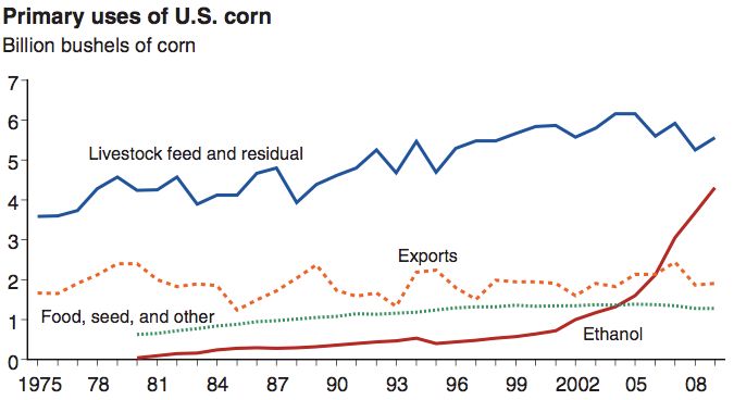
2.3 The Market for Corn
The demand for corn can be broken down into four components: food, feed for
livestock, exports, and ethanol. As Figure 2.2 represents, the non-ethanol uses of corn
have not altered significantly over the past decade, as greater ethanol production has
taken over a larger portion of total corn production (Wallander et al, 2011, 3).
The rise in ethanol production has had significant impacts on the market for corn.
In 2007, U.S. farmers planted 93.6 million acres of corn, the largest planting of corn since
1944 (Harrison, 2009, 493). The increase in corn planting is largely in response to
increased ethanol production. “Between 2000 and 2009, corn used for ethanol increased
by 3.7 billion bushels, while total corn production increased by 3.2 billion bushels”
(Wallander et al, 2011, 3). The increase in corn yields have not kept up with the growth
of ethanol production, creating a shortage. As a result, corn has exhibited historically
12high prices in recent years. In the 2007/ 2008 marketing years for corn, the farm level
price for corn averaged between $4.10-4.50 per bushel, a historic high (Harrison, 2009,
493). “The increasing demand for ethanol requires the use of large amounts of corn,
soybeans, sugarcane, or other crops to feed the large fermentation vats necessary for mass
production of ethanol fuel. The need for corn to produce much larger quantities of
ethanol has inflated prices from the generally stable price of $2 per bushel to more than
$4 by early 2007” (Luchansky and Monks, 2008, 2). Despite historically large corn
acreage and continuous advancements in corn yields, the surge in ethanol production has
increasingly taken corn away from its other, non-ethanol uses. As of 2002, ethanol
accounted for about 10% of total corn use (Anderson and Coble, 2010, 53). In 2007, this
percentage increased to 24% (Harrison, 2009, 493), and in 2009 this figure was estimated
to be around 30% (Anderson and Coble, 2010, 53). The proportion of corn use devoted to
ethanol production is increasing rapidly, while concurrent levels of non-ethanol corn use
have remained stable or declined, with the most notable decline in the feed component
(Anderson and Coble, 53). Corn’s use as feed for livestock has historically been the
largest component of corn’s demand. As ethanol production has been chipping away
from the corn devoted to feeding America’s livestock, meat and other livestock products
are becoming more expensive to produce.
13Figure 2.2: Primary Uses of U.S. Corn, 1975-2009
(Source: U.S. Department of Agriculture)
Corn as a Food Source
Corn plays a major role in the United States food market. In 1973, U.S. Secretary
of Agriculture, Earl “Rusty” Butz, revolutionized the American agriculture industry in
such a way that would establish “cheap corn” for decades to come (Pollan, 2006, 53).
With an abundance of cheap corn available, American food scientists would devise
unique ways to incorporate corn into our everyday diets.
Corn serves multiple purposes as a food source. The most obvious role that corn
plays as a food source is simply eating corn itself, although there are numerous other
ways that corn may find its way onto the dinner table. Corn is frequently transformed into
a handful of “food inputs”, the most common of which are cornstarch, corn syrup, and
high-fructose corn syrup. These goods produce a cheap dose of pure sweetness and fat,
and are commonly used in soft drinks and various junk foods (Duckworth, 2012, 1).
Lastly, the most indirect method that corn is transformed into food is as feed for cattle,
14pigs, and chickens. Being that corn prices have reached historically high levels, producers
of America’s meat supply have now passed on higher prices to consumers. Corn has
become such a large presence in America’s food industry that Michael Pollan (2006)
estimates that of the forty-five thousand items in the average American supermarket,
more than a quarter of them now contain corn (19). Given our reliance on corn as a food
source, we can expect that higher corn prices lead to food price inflation.
Harrison (2009) examines the “effects of biofuel production on commodity prices
and their transmission to retail food prices” (493). Much like Anderson and Coble
(2010), Serra et al. (2010), and Fortenbery et al. (2008) have all discussed in their
findings, the increased demand for corn-ethanol has affected corn prices in recent years.
Corn serves as feed for numerous commercial livestock and as an input in a several food
products, and therefore, we can expect that higher corn prices are likely to have some
effect on the retail food prices. Harrison (2009) cites a previous study that estimates that a
“30% increase in the price of corn, and associated increases in the prices of wheat and
soybeans, would increase egg prices by 8.1%, poultry prices by 5.1%, pork prices by
4.5%, beef prices by 4.1%, and milk prices by 2.7%” (499). The findings discussed by
Harrison imply that price inflation for the aforementioned food items are the result of
increased ethanol production due to higher oil prices. Harrison’s discussion is consistent
with that of related literature.
2.4 Obesity in America
America currently stands as the world’s most obese country, with roughly two-
thirds of Americans classified as either overweight or obese (Finkelstein and Zuckerman,
152008, xi). This onset of obesity has taken hold over the past three decades; the number of
obese individuals has more than doubled during this time (Finkelstein and Zuckerman,
2008, xi). Obesity increases the risk of a number of medical conditions (i.e. Type II
diabetes, hypertension, and high cholesterol) (Finkelstein and Zuckerman, 2008, 10). In
fact, poor diet and physical inactivity attributes to 15.2% of total U.S. deaths, the second
leading cause of death behind tobacco (Finkelstein and Zuckerman, 2008, 10). Given the
severity of obesity in America, the study of its causes and implications are worthwhile.
Finkelstein and Zuckerman (2008) argue that America’s economic growth is the
root cause of this problem, as technology has enabled lifestyles that are more sedentary
and our nation’s food industry increasingly allows us to consume more for our dollar.
Since 1982, healthy foods such as fruits and vegetables have become increasingly more
expensive relative to unhealthy foods such as fast food and junk food. Junk foods are
appealing to many people as they are a quick and immediate source of calories, although
not necessarily rich with nutrients. On the other hand, healthy foods such as fruits and
vegetables are high in nutrients, but have fewer calories. As corn acreage expands to
accommodate for increased ethanol production, the supply of fruits and vegetables is
likely to decline, thus raising prices. However, given corn’s extensive use as a food input,
ethanol production is expected to have a larger impact on the prices of “unhealthy foods”
relative to that of “healthy foods”.
2.5 Summary
In an effort to help diversify America’s energy sources and decrease our
dependence on finite fossil fuels, government mandates have greatly influenced the
16dramatic increase of ethanol fuel production over the past decade. The existing literature
provides ample reason to believe that a surge in ethanol production has contributed to
higher food prices in recent years. That being said, the analysis of this paper will examine
which types of food have been affected most by the evolution of the ethanol market. We
will look at the magnitude of relative price changes and its relationship to obesity. The
next chapter will provide an outline of our analytical approach and discuss the
econometric techniques used in our model.
17Chapter 3
Econometric Techniques and Analytical
Approach
This chapter begins with a detailed description of the approach we are using to
answer the question at hand. Given the various markets at play, our analytical approach
will be broken into three stages. Stage 1 will analyze the effects that ethanol production
has on corn prices. Stage 2 will test the relationship between corn prices and the relative
prices of “more” and “less” healthy foods as defined by Finkelstein and Zuckerman
(2008). The final stage will assess the effects that relative food prices have on obesity.
Stages 1 and 2 will utilize cointegration techniques, supplemented by Granger causality
tests. Stage 3, due to data limitations, will utilize ordinary least squares regression
analysis. The purpose of this chapter is to outline the reasons supporting this multiple-
stage model and provide an understanding of the econometric tools that being utilized.
3.1 Methodology
Time series data, like the data used in this study, are an important type of data that
are used regularly in economic analysis. Nevertheless, there are several obstacles to be
overcome when testing relationships between two or more time series variables.
One overarching problem when running regressions involving time series data is
that the assumption has been made that the underlying data are stationary (Gujarati, 2003,
792). That is, the data are assumed to have a mean and variance that do not vary
systematically over time (Gujarati, 2003, 26). Many time series data (e.g. GDP), exhibit a
18clear upward trend so to assume that the data are stationary naturally lends itself to some
problems. The main problem that we are concerned with in this study is that of spurious
regression results, in which two or more variables may exhibit a significant relationship
where in fact the relationship is due to some exogenous factor. One technique that can
protect against spurious results is cointegration. Much like the work of Serra et al. (210,
we will utilize cointegration testing in order to establish the existence of a long run
relationship between our chosen variables.
Cointegration
Cointegration testing will serve as the primary method of testing for significant
long run relationships in this analysis. By definition, “cointegration is a statistical
property of time series data in which two or more time series each share a certain type of
behavior in terms of their long run fluctuations” (Swedish Academy of Sciences). More
specifically, cointegration tests hypotheses and estimates relationships among
nonstationary variables. A variable is said to be nonstationary if it has no clear tendency
to return to a constant value or fluctuates around a linear trend (Swedish Academy of
Sciences). This phenomenon of nonstationarity may also be referred to as random walk.
Equation 1 below exhibits the random walk model.
Yt = Yt-1 + ut (1)
In this model, “suppose ut is a white noise error term with mean 0 and variance
2. The equation states that the series Yt is said to be a random walk if the value of Y at
19time t is equal to its value at time (t 1) plus a random shock” (Gujarati, 2003, 799). We
can further think of this equation as a regression of Y at time t on its value lagged one
observation period (Gujarati, 2003, 799). This lag in the random walk model makes the
cointegration technique very data intensive. Due to data limitations regarding obesity
measures, cointegration will only be used in Stages 1 and 2 of our analytical approach.
It is common for time series variables, such as the ones used in this analysis, to
develop stochastically, thus exhibiting random walk. The cointegration technique is
useful in that it protects against spurious results that ordinary least squares (OLS)
regression is susceptible to when using nonstationary variables. In an attempt to establish
cointegrating relationships in this paper, the methodology will be broken into two steps.
Step 1 will verify that each time series being analyzed is, in fact, nonstationary. Step 2 is
the performance of the cointegration test itself.
Step 1: The Unit Root Test
The unit root test is a popular test to determine stationarity, or in our case,
nonstationarity. To determine whether a time series is nonstationary, we can re-write our
random walk model from Equation 1 as
Yt = Yt-1 + ut -1 ≤ ≤ 1 (2
where ut is a white noise error term and is the coefficient of autocorrelation.
We know that if = 1, that is, in the case of a unit root, then Equation 2 becomes
the same random walk model as Equation 1, which we know exhibits a nonstationary
20process (Gujarati, 2003, 814). For testing purposes, we manipulate Equation 2 by
“subtracting Yt-1 from both sides of the equation to obtain:
Yt - Yt-1 = Yt-1 - Yt-1 + ut
= ( - 1) Yt-1 + ut
∆ Yt = Yt-1 + ut (3
where = and is the first difference operator” (Gujarati, 2003, 814. In the case
that = , Equation 3 will become
∆ Yt = (Yt - Yt-1 = ut (4
in which case the first differences of a random walk time series model are equivalent to
the error term, which we know is stationary (Gujarati, 2003, 814. In other words, if =
, then = 1, and the time series being tested is nonstationary (Gujarati, 2003, 814.
To test for nonstationarity, we must regress the first differences of Yt onto Yt-1 and
see if the estimated slope coefficient in this regression ( is zero or not (Gujarati, 2003,
814. In other words, we test the null hypothesis that = around a 95% confidence
interval. If we fail to reject the null hypothesis that is zero, then the time series Yt is
nonstationary and we say it is I (1. In order to be eligible for cointegration testing, each
time series being considered must be I (1.
21Step 2: Cointegration Testing
Once the unit root tests confirms that all variables at hand are I (1, we may
perform a cointegrating regression. Suppose then that we regress Yt on Xt as follows:
Yt = 1 + 2Xt + ut (5
where 1 is the intercept, 2 is the slope coefficient and ut is the white noise error term.
To determine if Yt and Xt are cointegrated (i.e. there exists a long run equilibrium
relationship between X and Y, the error term, ut, must be stationary. To do so, we re-
write Equation 5 and subject ut to unit root analysis.
ut = Yt 1 2Xt (6
If the error term is stationary, or I (, the difference between the two time series
at time t will remain relatively stable over time and “the two variables will exhibit a long-
term, or equilibrium, relationship between them” (Gujarati, 2003, 822. Graphically
speaking, the time series will appear to move together. As Gujarati notes, “this presents
an interesting situation, for although Yt and Xt are individually I 1, that is, they have
stochastic trends, their linear combination is I . So to speak, the linear combination
cancels out the stochastic trends in the two series” (Gujarati, 2003, 822. This testing of
the error term is the fundamental difference between ordinary least squares regression
analysis and cointegration regression analysis.
22Granger-Causality Test
Once cointegrating relationships are established, the Granger causality test will be
used to augment our analysis.
At the heart of econometric analysis lies the motive to determine one variable’s
dependence on other variables. But as we know, a relationship (or even cointegrating
relationship among variables does not imply causality or direction of influence (Gujarati,
2003, 696. For instance, X may be driving Y to change, but not the other way around.
This notion of causality is an important topic when dealing with time series data.
Causality becomes an important issue with time series data simply because time
only moves in direction, forward. “That is, if event A happens before event B, then it is
possible that A is causing B. However, it is not possible that B is causing A. In other
words, events in the past can cause events to happen today. Future events cannot”
(Gujarati, 2003, 696. Suppose we are interested in the direction of causality between two
time series, Yt and Xt. The Granger causality test can then be summarized by the
estimation of the following two regressions:
Yt = i Xt-i + j Yt-j + u1t (7
Xt = i Xt-i + j Yt-j + u2t (8
where u1t and u2t are uncorrelated (Gujarati, 2003, 697.
Equation 7 suggests that the current value of Yt is related to past values of itself
as well as values of Xt. The reciprocal of this statement is true for Equation 8. In short,
23the results will show that Xt causes Yt if I ≠ from Equation 7 and j = from
Equation 8 when tested for significance. The Granger causality test will play a part in our
model as it provides more insightful findings. The econometric methods of this paper
have been outlined and we will now turn towards the data that will be used in this study.
3.2 Data
The data used were taken from a number of different sources and come in various
time series and units.
Stage 1 of our analytical approach uses monthly corn and ethanol prices as
reported by the U.S. Department of Agriculture (USDA). Corn prices are quoted in
dollars per bushel and ethanol prices are quoted in dollars per gallon. The time period for
the first stage of the model ranges from January of 1982 to May of 2011. This is an
appropriate time period since ethanol production remained small throughout the 1980’s,
exhibited small growth over the 1990’s, and then boomed in the mid 2000’s. This dataset
utilizes the most recent data, and thus, it captures all trends of corn and ethanol prices that
are relevant to the purpose of this paper.
Stage 2 uses monthly corn prices, monthly prices of meat products (beef, pork,
poultry, and fish) and the monthly prices of “more” and “less” healthy foods. Corn prices
were taken from the USDA whereas meat prices and relative food prices are comprised of
various consumer price indexes (CPI) taken from the Bureau of Labor Statistics. The CPI
indexes for relative food prices have been grouped into the two previously mentioned
food categories. “Healthy foods” consists of the non-seasonally adjusted CPI for Fruits
and Vegetables, for all urban consumers. “Unhealthy foods” is comprised of the
24following non-seasonally adjusted CPIs for all urban consumers: Sugars and Sweets, Fats
and Oils, Other Foods, and Non-alcoholic Beverages. The index produced by the
grouping of these indexes is the sum of a weighted average according to each category’s
relative importance as of November 211. The aforementioned classification for
“healthy” and “unhealthy” foods was that of Finkelstein and Zuckerman (2008), adjusted
slightly due to data availability. The time period for this stage of the model is once again
January of 1982 to May of 2011 in order to remain consistent with the first stage of the
model.
The final stage will consist of annual prices of meat products, “healthy” and
“unhealthy” foods and annual data that report the percentage of the U.S. population with
a body mass index (BMI) above 30. “Body mass index is calculated by taking an
individual’s weight in kilograms divided by height in meters squared (BMI = kg/ m2)”
(Finkelstein and Zuckerman, 2008, 7. A BMI between 30 and 35 is classified as obese,
whereas anything over 35 is consider very obese. BMI aims at measuring body fat, and
while not completely accurate, it is widely regarded as a reliable proxy. The BMI data
was taken from the Center for Disease Control and is only available on an annual basis
from 1995-2010. To supplement our analysis, we will also use data regarding the prices
of McDonald’s “Big Mac” taken from the The Economist’s: Big Mac Index.
3.3 Analytical Approach
As previously mentioned, the analytical approach for this study will comprise of
three stages. Each stage aims at establishing a particular relationship between two
variables. Once the targeted relationship has been verified, we will move on to the next
25stage of the analytical approach. The ultimate goal of our approach is to examine any
existing relationship that U.S. corn ethanol production has with America’s obesity
epidemic. The analytical approach is segmented as follows:
Stage 1: Ethanol Prices and Corn Prices
Stage 1 will concentrate on the relationship between an increase in U.S. corn
ethanol production and U.S. corn prices.
In response to escalating demand in the past decade, ethanol production has
nearly doubled between 22 and 25 alone (Cooper, 1. However, demand for non-
ethanol corn use has remained steady (Cooper, 2). While technological advances have
enabled historically high corn yields, it has not been enough to fully meet the needs of the
emerging ethanol industry. Consequently, corn is being taken away from its traditional
non-ethanol uses in order to fuel ethanol’s needy demand. Because the overwhelming
majority of U.S. ethanol is derived from corn, we expect that a linkage exist between the
two markets. The rising demand for ethanol would trigger a boom in corn demand,
ethanol’s primary input. Corn’s rising demand is exceeding its supply, thus driving higher
corn prices (Wallander et al, 2011, 3. A visual depiction of corn and ethanol prices from
1982.01-2011.05 is shown in Figure 3.1. It is interesting to note that since the mid-
2’s, corn prices have been on a dramatic upward trend. The timing of this price
increase coincides with the ethanol boom.
Given the aforementioned scenario in the U.S. agriculture industry, we would
expect a significant long-run relationship to exist between ethanol production and corn
prices. Stage 1 of our analytical approach is inspired by the work of Serra et al. (2010) in
26which cointegrating techniques are used to model the relationships between the prices of
corn, ethanol, oil and gasoline. As their results suggests, there is a long-run
(cointegrating) relationship between food and energy prices (i.e. corn and ethanol). The
purpose of this stage of the model is to reproduce the findings of Serra et al. (2010) and
update their work with more recent data. Our cointegration model will use monthly
ethanol prices as the independent variable and monthly corn prices as the dependent
variable. Note, however, that such cointegrating relationships do not imply causation in
any direction. Therefore, in addition to recreating the work of Serra et al. (2010) we will
perform the Granger causality test to determine if ethanol production is in fact driving
corn higher prices in recent years as the literature suggests. If a cointegrating relationship
between ethanol prices and corn prices is confirmed, we will move to Stage 2 of our
analytical approach, in which we diverge from the energy industry and focus on the role
that corn plays in the U.S. food market.
7
6
5
4
$
3
2
1
0
82 84 86 88 90 92 94 96 98 00 02 04 06 08 10
CORN ETHANOL
Figure 3.1: Monthly Corn and Ethanol Prices, 1982.01-2011.05
(Source: U.S. Department of Agriculture
27Stage 2: Corn Prices and Food Prices
Stage 2 will examine the effect that corn prices have on both meat prices and
relative food prices.
Michael Pollan (2006) reports that about 60 percent of America’s corn crop goes
to feeding livestock (Pollan, 66). Meat, while high in protein and B-vitamins, contains
high levels of fat and cholesterol. Excess consumption of meat has the potential to
contribute to obesity. Given corn’s integral role in feeding America’s livestock, a
statistical analysis of their relationship is worthwhile
For several decades now, corn has played an integral role in America’s food
industry as modern food science has extended corn’s breadth far beyond the traditional
consumption method of just “corn on the cob”. Given corn’s presence in the U.S. food
market, Stage 2 aims to examine the relationship between corn prices and relative prices
of “more” and “less” healthy foods. This stage of the model serves as an intermediate
step that links the energy market to America’s obesity epidemic.
The work of Finkelstein and Zuckerman (2008) reveals that relative price
differences between “more” and “less” healthy foods may have a substantial impact on
American obesity figures. That being said, relative food prices are used in this phase of
the model as a segue from the corn market to the food market. As Figure 3.2 and Figure
3.3 clearly show, there has been a growing disparity between “healthy” and “unhealthy”
foods since the late 1980’s.
28Fresh fruits and vegetables are typically low in calories, yet they offer consumers
with bountiful nutrition in the form of vitamins and minerals. Should Americans choose
to engage in a vegetarian diet, they are likely to experience health benefits. It is for this
320
280
240
CPI
200
160
120
80
82 84 86 88 90 92 94 96 98 00 02 04 06 08 10
UNHEALTHY HEALTHY
Figure 3.2: CPI of “Healthy” and “Unhealthy” Foods, 1982.01-2011.05
(Source: Bureau of Labor Statistics)
reason that fruits and vegetables have been categorized as “healthy” foods. Conversely,
food items categorized as “unhealthy” are high in calories, yet they lack significant
nutritional value. Several of the foods within the “unhealthy” category have been
processed, packaged, or in some way modified. “Foods more dependent on technology
are often those with the greatest amounts of added sugars and fats and therefore the
highest in calories” (Finkelstein and Zuckerman, 2008, 23). Their comparison reveals that
it has become more expensive for Americans to consume healthier foods and
comparatively less expensive for them to consume unhealthier foods. For the millions of
Americans living on a tight budget, “unhealthy” foods have become the cheapest
immediate source of energy they can get (Finkelstein and Zuckerman, 2008, 8.
29As Pollan (2006) points out, corn production has historically been a beneficiary of
massive government subsidies, as U.S. policy has targeted low corn prices since 1973
(Pollan, 52). Due to corn’s increasing presence in the processed food industry, there is
HEALTHY/UNHEALTHY
1.6
1.5
1.4
1.3
CPI
1.2
1.1
1.0
0.9
82 84 86 88 90 92 94 96 98 00 02 04 06 08 10
Figure 3.3: Relative Prices of “Healthy” and “Unhealthy” Foods, 1982.01-2011.05
(Source: Bureau of Labor Statistics)
reason to believe that corn plays a major role in relative food prices. It is interesting to
note that in Figure 3.3 relative food prices have trended downwards since 2008, perhaps a
result of the additional 3.7 billion bushels of corn devoted to ethanol from 2000-2009
(Wallander et al, 2011, 3). We hypothesize that rising corn prices have raised the price of
“unhealthy” foods, thus lowering relative food prices in recent years.
Using relative food prices as the dependent variable and corn prices as the
independent variable, Stage 2 will use cointegration testing to determine if a significant
long-run relationship exists between the two variables. Similar to Stage 1, the Granger
causality test will then be applied to determine if corn prices are in fact driving relative
food prices as we hypothesized. If a cointegrating relationship exists between corn prices
30and relative food prices, Stage 3 of our analytical approach will model the relationship
between meat prices and obesity, as well as, relative food prices and obesity.
Stage 3: Food Prices and Body Mass Index
The final phase of our analytical approach will assess the relationship between
meat prices, relative food prices and the percentage of the U.S. population categorized as
“obese” according to BMI reports. Since about the 196’s America has witnessed a
steady rise in the number of people that are obese (See Figure 3.4). In recent years,
roughly one in every three Americans can be labeled as obese. The existing literature,
primarily that of Finkelstein and Zuckerman (2, provides us with ample reason to
believe that relative food prices play a major role in the current obesity epidemic. The
law of demand would have us believe that the cheaper food is the more of it we consume,
precisely the situation we have faced for the past four decades. “Since 196, the relative
price of food compared with other goods has decreased by about 16% percent. Since
1978, food prices have dropped 38 percent relative to the prices of other goods and
services” (Finkelstein and Zuckerman, 2008, 21. However, it is not just that food in
general has become cheap, it is the types of food that have become cheap. Compared with
healthy foods such as fruits and vegetables, energy dense foods have become increasingly
cheaper, as illustrated by Figure 3.2. Between 1983 and 25, the price of fruits and
vegetables has risen 19 percent, whereas foods such as fats and oils, sugars and sweets,
and non-alcoholic beverages have risen by much smaller amounts7 percent, 66
percent, and 32 percent respectively (Finkelstein and Zuckerman, 2008, 21. Such price
adjustments for food have not only shifted consumption towards “unhealthy” foods, but it
31has increased typical portion sizes as well. A 2-oz soda has replaced the once typical 8-
oz version, snacking has become a standard activity between meals, and the term
“supersize me” has grown to be a common American colloquialism (Finkelstein and
Zuckerman, 2008, 22). It should be noted too that even slight caloric imbalances could
lead people to become obese over time. Finkelstein and Zuckerman (28 estimate that
OBESITY
28
26
24
22
20
18
16
14
95 96 97 98 99 00 01 02 03 04 05 06 07 08 09 10
Figure 3.4: Percentage of U.S. Population that is Obese, 1995-21
(Source: Center for Disease Control
eating just 1 extra calories a day could generate an average gain of 1 lbs per year.
This fragile maintenance of the recommended 2,5 calories-a-day diet could be swiftly
violated by just 4 Hershey’s Kisses, 2 Oreo cookies, 1 French fries, an 8-oz Coca-Cola,
or 1 tablespoon of peanut butter (Finkelstein and Zuckerman, 2008, 19. While there are
certainly numerous other factors that influence obesity (i.e. socioeconomic status,
physical activity, genetic makeup, etc., the existing literature confirms that relative food
prices seem to be among the most prominent. It is for these reasons that relative prices of
32“more” and “less” healthy foods and BMI data will be modeled in this final phase of the
model.
Stage 3 of the analytical approach attempts to provide the answer to the ultimate
question of this study: Does an increase in U.S. corn ethanol production cause Americans
to eat healthier? BMI data is a relatively recent attempt at quantifying obesity, and thus,
its availability is limited. This stage will look at food prices and the percentage of
Americans that are “obese” from 1995-21 on an annual basis. Due to the small sample
size, cointegration testing would be invaluable, so ordinary least squares regression
analysis will be performed instead. In the next chapter, we will present and analyze our
empirical findings.
33Chapter 4
Analysis of Empirical Results
This chapter presents the findings of the econometric analysis as outlined in the
previous chapter. Corresponding to the structure of our analytical approach, the results
are introduced in three stages. The first section discusses the relationship between ethanol
prices and corn prices. The second section discusses the relationship between corn prices
and food prices, while the third section discusses the relationship between food prices and
obesity.
4.1 Stage 1: Ethanol Prices vs. Corn Prices
Stage 1 of our analytical approach examines the relationship between U.S. ethanol
prices and U.S. corn prices.
Unit Root Tests
As mentioned in Chapter 3, cointegration techniques pertain to testing
relationships among nonstationary variables. Therefore, prior to estimating cointegration
equations, each variable being used must submit to a unit root test to confirm that it is in
fact nonstationary. Stage 1 uses two variables, the monthly price per gallon of ethanol
and the monthly price per bushel of corn received by U.S. corn farmers.
The estimated p-value for ethanol and corn prices was .17 and .62 respectively
(Appendix B, Table 2. Both values are not significant at the 5% level, and thus, we fail
to reject the null hypothesis that the variable has a unit root. In other words, both ethanol
and corn prices are nonstationary and are eligible for cointegration testing.
34You can also read