Formation of glacier tables caused by differential ice melting: field observation and modelling
←
→
Page content transcription
If your browser does not render page correctly, please read the page content below
The Cryosphere, 16, 2617–2628, 2022
https://doi.org/10.5194/tc-16-2617-2022
© Author(s) 2022. This work is distributed under
the Creative Commons Attribution 4.0 License.

Formation of glacier tables caused by differential ice melting:
field observation and modelling
Marceau Hénot1 , Vincent J. Langlois2 , Jérémy Vessaire1 , Nicolas Plihon1 , and Nicolas Taberlet1
1 Laboratoire
           de Physique, Université de Lyon, ENS de Lyon, Université Claude Bernard Lyon 1, CNRS, 69342 Lyon, France
2 Laboratoire
           de Géologie de Lyon, Terre, Planètes, Environnement, Université Claude Bernard Lyon 1,
ENS de Lyon, Université Jean Monnet, CNRS, 69100 Villeurbanne, France

Correspondence: Nicolas Taberlet (nicolas.taberlet@ens-lyon.fr)

Received: 20 September 2021 – Discussion started: 11 October 2021
Revised: 27 May 2022 – Accepted: 1 June 2022 – Published: 29 June 2022

Abstract. Glacier tables are structures frequently encoun-         rock thickness, its aspect ratio, and the ratio between the av-
tered on temperate glaciers. They consist of a rock supported      eraged turbulent and short-wave heat fluxes.
by a narrow ice foot which forms through differential melt-
ing of the ice. In this article, we investigate their forma-
tion by following their dynamics on the Mer de Glace (the
Alps, France). We report field measurements of four specific       1   Introduction
glacier tables over the course of several days, as well as snap-
shot measurements of a field of 80 tables performed on a           A wide variety of spectacular shapes and patterns formed
given day. We develop a simple model accounting for the            through differential ablation can be found in nature: sur-
various mechanisms of the heat transfer on the glacier us-         face patterns known as rillenkarren result from the disso-
ing local meteorological data, which displays a quantitative       lution of soluble rocks (Cohen et al., 2016, 2020; Claudin
agreement with the field measurements. We show that the            et al., 2017; Guérin et al., 2020), tafoni are cavernous rock
formation of glacier tables is controlled by the global heat       domes dug by salt crystallization during wetting–drying cy-
flux received by the rocks, which causes the ice underneath        cles (Huinink et al., 2004), scallops and sharp pinnacles are
to melt at a rate proportional to the one of the surrounding       created by convective flows (Huang et al., 2020; Weady et
ice. Under large rocks the ice ablation rate is reduced com-       al., 2022), mushroom rocks undergo erosion of their base
pared to bare ice, leading to the formation of glacier tables.     by strong particle-laden winds (Mashaal et al., 2020), and
This thermal insulation effect is due to the warmer surface        hoodoos consist of a hard stone protecting a narrow column
temperature of rocks compared to the ice, which affects the        of sedimentary rock from rain-induced erosion (Young and
net long-wave and turbulent fluxes. While the short-wave ra-       Young, 1992; Bruthans et al., 2014; Turkington and Paradise,
diation, which is the main source of heat, is slightly more        2005).
absorbed by the rocks than the ice, it plays an indirect role in      On ice and snow surfaces, similar structures can be found:
the insulation by inducing a thermal gradient across the rocks     slender snow blades known as penitentes (Mangold, 2011;
which warms them. Under a critical size, however, rocks can        Bergeron et al., 2006; Claudin et al., 2015), as well as blue
enhance ice melting and consequently sink into the ice sur-        ice ripples observed in Antarctica (Bintanja et al., 2001)
face. This happens when the insulation effect is too weak          and on Mars (Bordiec et al., 2020), are caused by sublima-
to compensate for a geometrical amplification effect: the ex-      tion; suncups are bowl-shaped depressions found at the sur-
ternal heat fluxes are received on a larger surface than the       face of a snow patch (Rhodes et al., 1987; Betterton, 2001;
contact area with the ice. We identified the main parameters       Mitchell and Tiedje, 2010); scallops are regularly spaced
controlling the ability of a rock to form a glacier table: the     patterns of surface indentations at the ice–water or ice–
                                                                   air interface (Bushuk et al., 2019); ice sails (or pyramids)
                                                                   are larger bare-ice structures that form on debris-covered

Published by Copernicus Publications on behalf of the European Geosciences Union.
2618                                              M. Hénot et al.: Formation of glacier tables caused by differential ice melting

Figure 1. (a–c) Formation of a natural granite glacier table (rock 1;
see Table 1).

glaciers (Evatt et al., 2017; Fowler and Mayer, 2017); Zen
stones found on frozen lakes are pebbles resting on a delicate
ice pedestal protected from sun-induced sublimation (Taber-             Figure 2. (a) Map of the Mer de Glace in the French Alps (Google
let and Plihon, 2021); and glacier tables (see Fig. 1c) form            Earth image © 2021 Maxar Technologies) locating the measure-
when a foot of ice resists melting due mostly to thermal                ment site of 3 June 2021 (1), the time-lapse observation sites of
insulation provided by a large rock (Agassiz, 1840; Bouil-              June 2021 (2) and June 2019 (3), and the Requin AWS (4). (b) The
lette, 1933, 1934; Smiraglia and Diolaiuti, 2011; Hénot et              3D schematics of a typical glacier table defining the height H (t) of
al., 2021).                                                             the ice foot and the average thickness h and widths d1 and d2 of
   On a temperate glacier, the ice ablation rate is influenced          the rock. (c) Picture of a portion of the glacier taken in June 2021
                                                                        showing natural glacier tables, from which the data shown in Fig. 3
by the presence of debris on its surface. Indeed, a dense de-
                                                                        were obtained.
bris layer covering an ice surface can, when thin enough (less
than 0.5 cm), enhance the ice melting compared to a bare-ice
surface or, if thick enough, act as an insulation layer and re-         tyre, 1984). In a previous work (Hénot et al., 2021), artifi-
duce the melting rate (Östrem, 1959). The insulation effect is          cial glacier tables were reproduced experimentally in a lab-
well captured by complex energy balance models which use                controlled environment (constant temperature, humidity, ab-
meteorological data as input parameters (Reid and Brock,                sence of wind), at a centimetric scale. The study focused on
2010; Collier et al., 2014) and more recently by enhanced               the initial behaviour of pattern formation using cylindrical
temperature index models (Carenzo et al., 2016; Moeller et              “rocks” of various sizes, the aspect ratio and materials, ini-
al., 2016). The melt amplification effect for thin debris layers        tially resting on a flat ice surface. Although this small-scale
has been explained by its patchiness (Reid and Brock, 2010)             study under controlled conditions allowed one to understand
or by its porosity to airflow (Evatt et al., 2015). At a more           the physical mechanisms that could play a role in glacier ta-
local scale, patches of dirt or ashes on a glacier are known to         ble formation, it did not encompass the complexity of the
lead to the formation of ice structures known as dirt cones,            energy balance on a natural glacier, in particular the effects
which consist of ice cones covered with a centimetric layer of          of the direct solar irradiation and of the wind.
dirt (Swithinbank, 1950; Krenek, 1958; Drewry, 1972; Bet-                  In this article, we report field observations made on the
terton, 2001).                                                          Mer de Glace (French Alps) of the formation dynamics of
   Glacier tables (see Fig. 1c) are structures frequently en-           glacier tables monitored over the course of a few days, as
countered on the levelled part of temperate glaciers (Agassiz,          well as a systematic measurement of already-formed tables
1840). They typically consist of a metre-sized rock supported           on a given day. The Mer de Glace is a temperate glacier,
by a column (or foot) of ice. They form over the course of a            meaning that the ice temperature is always given by the melt-
few days to a few weeks at the end of the spring, from May              ing temperature of water: Tice = 273 K. We use local meteo-
to June, and may progressively disappear during the sum-                rological data to fit the ice ablation rate and characterize the
mer. Very large tables however, whose size can reach 10 m,              heat transfer mechanisms at the surface of the glacier. We
can last for several years (Bouillette, 1933, 1934). Glacier            then develop a 1D conduction model taking into account the
tables form because the ablation rate of the ice is lower un-           effect of the solar irradiation as well as sensible and long-
der the rock than at the air–ice interface. When the ice foot           wave heat fluxes, which is in excellent agreement with the
becomes too thin, the table falls, usually on its south side.           field measurements and which illustrates the synergistic ef-
The ice foot progressively disappears, and the rock can po-             fect between solar irradiation and sensible flux responsible
tentially form another table if it is not too late in the sea-          for glacier table formation.
son. Similarly to what is known for debris layers, smaller
rocks tend not to form tables but can instead increase the
melting rate and gradually sink into the ice, creating narrow
and deep holes which can reach up to 15 cm in depth (McIn-

The Cryosphere, 16, 2617–2628, 2022                                                          https://doi.org/10.5194/tc-16-2617-2022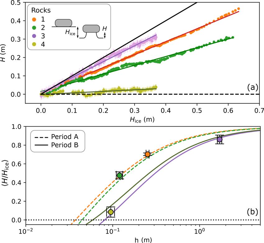
M. Hénot et al.: Formation of glacier tables caused by differential ice melting 2619
2 Observation
2.1 Location and definitions
In this article, we report two sets of observations made on
the Mer de Glace: a time-resolved camera recording of the
formation and evolution of four glacier tables and a field ob-
servation of 80 glacier tables.
The lower part of the Mer de Glace (below a 2100 m alti-
tude) is largely covered with granitic debris, with sizes rang-
ing from submillimetric up to several metres. In the follow-
ing, their dimensions are characterized by their thickness h
and their larger and smaller widths d1 and d2 (see Fig. 2b).
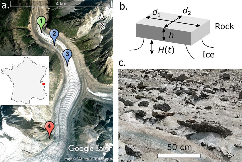
We define an effective width of the rock deff = 2d1 d2 /(d1 + Figure 3. Raw data of the observation made at location 1 (see
d2 ), whose expression will be justified in Sect. 3.2, and the Fig. 2a) on 3 June 2021: height of the ice foot (H > 0) or of the
aspect ratio β = h/deff . The vertical distance from the bot- penetration depth of the rock in the ice (H < 0) as a function of the
tom of a rock to the surface of the ice far from it is denoted rock thickness h (a) and widths d1 and d2 (b). On the date of these
observations the rocks were still standing on their ice feet and the
H . This quantity is either positive if the rock forms a table,
maximum heights had presumably not been reached yet.
in which case it corresponds to the height of the ice foot, or
negative if the rock sinks into the ice surface, in which case
it corresponds to the depth of the hole. 45.8846◦ N, 06.9297◦ E; see marker 4 in Fig. 2a), 600 m
higher than and 3 km away from the measurement site. The
2.2 Time evolution of four large tables time resolution was 1 h in 2019 and 15 min in 2021. During
a 2-week time period in July 2021, we also measured the air
Time-lapse images were obtained using an autonomous temperature at location 2, 3 m above the glacier surface (see
solar-powered camera (Enlaps Tikee) placed on three 1.5 m the Supplement), which was systematically 2.5 ◦ C higher
long wood rods set into the ice. Pictures (4608 px × 3456 px) than the AWS data. In the rest of the article, we use the AWS
were taken every 30 min between 05:00 and 22:00 (LT, data, to which an offset was added: Ta = Ta AWS + 2.5 ◦ C.
UTC+2) over 5 to 7 d until the camera fell on the ice due We do not expect the measured solar flux and the wind
to the melting around the supporting rods. The movements speed to be significantly affected by the distance from the
of the device were corrected by tracking two fixed points on measurement site. The incoming long-wave radiation com-
the background of the images. The positions of the top of ing from the atmosphere QLW atm ↓ was obtained from the
the rocks were then manually pointed onto each image. The S2M (SAFRAN–SURFEX/ISBA–Crocus–MEPRA) reanal-
formation of glacier tables created by four granite rocks of ysis, which combines information from numerical weather
various shapes and dimensions was recorded in two time pe- prediction models and in situ meteorological observation to
riods: A (7–14 June 2019) and B (4–9 June 2021), situated at estimate massif-averaged meteorological data with a 1 h time
locations 3 and 2 respectively on the map of Fig. 2a, as sum- resolution (Vernay et al., 2022a) (the parameters used to
marized in Table 1. Rocks 1, 2 and 4 were moved on clean, compute the meteorological data in this study are the closest
flat ice, in front of the camera, the day before the recording available that are representative of the real field, i.e. massif 3,
started in order to provide a controlled initial state in which 2100 m altitude, 20◦ slope facing north). The meteorological
the rocks are lying on a horizontal ice surface (H = 0; see data are displayed in Fig. 4c–l.
Fig. 1a). Rock 3 was already standing on an ice foot, ap-
proximately 1 m high, at the beginning of period B (see the 2.3 An 800 m2 field comprising 80 glacier tables
Supplement). The evolution of the vertical position of these
rocks is plotted in Fig. 4a and b. The position of the ice sur- On 3 June 2021, we systematically measured, in an area of
face was followed using a scaling rod, embedded into the ice 10 m × 80 m located at point 1 in Fig. 2a, the dimensions
and located approximately 2 m away from the rocks. of granite rocks (thickness and widths) as well as either the
The surface temperature of rock 4 was measured every height of the ice foot supporting them (H > 0) or the depth
5 min during period B using thermocouples and a homemade of penetration in the ice (H < 0). The data of H are plotted
battery-powered device (Arduino MKR ZERO and EVAL- in Fig. 3 as a function of the thickness h and the widths d1
CN0391-ARDZ Shield). The wind speed ua , air temperature and d2 of the rocks.
Ta , air specific humidity qa and solar radiative flux 8 were
measured at the Requin automatic weather station (AWS)
(see Nadeau et al., 2009, who use identical devices, for a
detailed description), at zm = 5 m above ground (located at
https://doi.org/10.5194/tc-16-2617-2022 The Cryosphere, 16, 2617–2628, 2022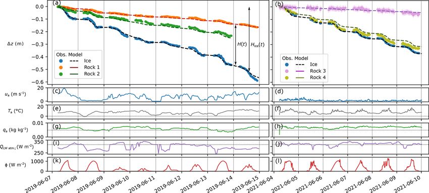
2620                                                M. Hénot et al.: Formation of glacier tables caused by differential ice melting

Table 1. Characteristics of the rocks studied.

                        Rock                                              Period of
                                  Location       Altitude   GPS coord.                     h (m)    d1 /d2 (m)         β
                        index                                             observation
                        1                                   45.9095◦ N,   A:                 0.25    1.21/0.98       0.23
                                      3          2020 m
                        2                                   06.9384◦ E    7–14 June 19       0.12    0.41/0.35       0.32
                        3                                   45.9168◦ N,   B:                 1.7       3.5/3.5       0.49
                                      2          1910 m
                        4                                   06.9319◦ E    4–9 June 21      0.095     0.32/0.31       0.30

Figure 4. (a, b) Vertical position of the ice surface (blue markers) and of rocks 1 to 4 (coloured markers; see Table 1). The dashed black line
corresponds to the model for ice ablation (see Sect. 3.1). The coloured solid lines correspond to the model for rocks (see Sect. 3.2). These
models use meteorological data measured at the Requin AWS as input: wind speed ua (c, d), air temperature Ta (e, f), air specific humidity
qa (g, h) and solar radiation 8 (k, l) as well as the long-wave radiation coming from the atmosphere QLW atm ↓ obtained from the S2M
reanalysis (i, j). The dotted lines correspond to the ice surface values. The date format is year-month-day.

3     Model                                                               and 8 is the incoming solar radiative flux (direct and diffuse)
                                                                          given by the meteorological S2M reanalysis model. The net
3.1    Energy balance at the ice surface                                  long-wave flux comes from a balance between the radiation
                                                                          received by the ice from the atmosphere QiLW atm ↓ and the
In the following, we characterize the heat flux balance on
                                                                          radiation emitted by the ice QiLW ↑ at temperature Tice . As-
the glacier surface by linking the ablated ice thickness to lo-
cal meteorological data in the same way as it has previously              suming an emissivity equal to unity 1, QiLW ↑ = σ Tice
                                                                                                                               4 , where
                                                                                          −8      −2  −4
been carried out in the literature (Hock, 2005; Conway and                σ = 5.67 × 10 W m K , is the Stefan–Boltzmann con-
Cullen, 2013; Fitzpatrick et al., 2017). The net incident heat            stant. This leads to QiLW = QLW atm ↓ −σ Tice
                                                                                                                      4 . The long wave
                                                                                                                i
                                                                          flux received from the atmosphere QLW atm ↓ is given by the
flux causing the glacier surface to melt with an open environ-
ment can be expressed as                                                  meteorological S2M reanalysis model. The turbulent fluxes
                                                                          transmitted to a surface are assumed to be proportional to the
Qopen env.→ice = QiSW + QiLW + QiH + QiE + QiR ,                  (1)     wind velocity ua :

where QiSW and QiLW are the net short-wave and long-wave                  QiH = ρa cp CH ua (Ta,zm − Tsurface ),                           (2)
radiative fluxes, QiH and QiE are the turbulent heat fluxes cor-          QiE   = ρa Lv CE ua (qa,zm − qsurface ),                         (3)
responding to sensible and latent heat respectively, and QiR is
the flux associated with rain. The short-wave radiation (when             where ρa = 0.98 kg m−3 is the air density at atmo-
neglecting the reflected radiation by the surrounding terrain)            spheric pressure at a 2100 m altitude patm = 785 hPa, cp =
is given by QiSW = 8(1 − αice ), where αice is the ice albedo             1004 J K−1 kg−1 is the specific heat capacity of air, Lv =

The Cryosphere, 16, 2617–2628, 2022                                                             https://doi.org/10.5194/tc-16-2617-2022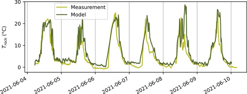
M. Hénot et al.: Formation of glacier tables caused by differential ice melting                                                   2621

2.48 MJ kg−1 is the latent heat of evaporation for water, and         this has little effect on the total heat transfer. The top and
Ta,zm and qa,zm are the air temperature and specific humid-           bottom areas are thus Atop = Abottom = d1 d2 , and the side
ity respectively at the height zm above the surface. Assum-           area is Aside = 2(d1 + d2 )h. (2) The surface temperature of
ing saturation near the melting ice surface, the specific hu-         the rock is assumed to be homogeneous and is denoted as
midity is qsurface = qice and is given by 0.622pvap (Tice )/patm ,    Trock , allowing the development of a 1D thermal conduction
where pvap (Tice ) = 611 Pa is the vapour pressure of water at        model. (3) The thermal process is assumed to be quasi-static,
temperature Tice (here and in the following, pvap (T ) values         meaning that all transient thermal effects are neglected. The
are obtained following the ITS-90 formula for water; Hardy,           validity of this assumption is discussed in the Supplement.
1998). The exchange coefficients CH and CE are assumed to                The energy balance of a rock, taking into account its 3D
be identical and are given by the simplest form found classi-         structure, is summarized in the schematic of Fig. 5a. The
cally in the literature assuming a neutral atmospheric stability      short-wave radiative flux is received by the rock on a surface
(Conway and Cullen, 2013):                                            hAsun i. This area should depend on the shape and orienta-
                                                                      tion of the rock with respect to the course of the sun, but for
                   k2
CH = CE =                    ,                                 (4)    the sake of simplicity in the following it is simply assumed
              (ln(zm /z0 ))2                                          to be equal to the rock base surface area hAsun i = Abase (the
where k = 0.41 is the von Kármán constant and z0 is a rough-          validity of this assumption is discussed in the Supplement).
ness length characterizing the surface (assumed to be equal           The long-wave flux coming from the atmosphere QLW atm ↓
for the momentum, temperature and vapour pressure). This              is also assumed to be received only on the top surface of
length is denoted as z0 ice for the ice surface. There was no         area Abase , but the rock also receives a long-wave flux on
precipitation and thus no associated heat flux on the glacier         its side denoted as QLW env ↓ . Strictly speaking, this quan-
during the duration of our study (QiR = 0). As the incoming           tity depends on the emissivity, surface temperature and view
heat flux directly causes the ice to melt, the vertical position      factor of all surfaces (ice, other rocks, terrain) seen from the
of the ice surface zice (t) and the total ablated thickness of ice    rock sides (Lienhard, 2019) and thus cannot be simply es-
since t = 0, Hice (t), are given by                                   timated. In the following it will be kept as an adjustable pa-
zice (t) − zice (0) = −Hice (t) =                                     rameter. The rock also emits a long-wave flux QrLW ↑ from its
                                                                      external surface (top and side). The sensible and latent fluxes
                          Zt                                          QrH + QrE are received from the air on the external surface of
                 − Lfus        Qopen env.→ice (t)dt,           (5)    the rock (of area Abase + Aside ). Finally a flux Qrock→ice is
                          0                                           transferred to the ice through the contact area Abase .
where Lfus = 303 MJ m−3 is the volumetric enthalpy of fu-                The quasi-static assumption implies that the flux balance
sion for ice. This model relies on meteorological data and has        is verified at each time t:
two adjustable parameters: the ice surface roughness z0 ice           Abase Qrock→ice = Atop QrSW
and its albedo αice . These adjustable parameters will be de-                             + Abase QLW atm ↓ − QrLW ↑

termined from the model fit to the ice ablation rate measured
                                                                                          + Aside QLW env ↓ − QrLW ↑

away from the glacier tables in Sect. 4.1.
                                                                                          + (Abase + Aside )(QH + QE ).             (6)
3.2   Glacier table formation model
                                                                      The net short-wave flux is QrSW = (1 − αrock )8 where
In Hénot et al. (2021), an analytical model was developed in          αrock = 0.18 is the albedo of the granite rock (measured by
order to explain the formation of artificial glacier tables made      Watson, 1971; see the Supplement). The granite emissiv-
of cylindrical caps in a controlled environment, in which the         ity is taken as equal to 1 (Michalski et al., 2004), leading
heat transfer (natural convection of air and infrared radiation       to QrLW ↑ = σ Trock
                                                                                        4 . The turbulent fluxes are computed ac-

from the enclosure) was modelled through an effective heat            cording to an equation similar to Eq. (3), for which the sur-
exchange coefficient. In the following, we adapt this model           face terms are those relative to the rock; i.e. Tsurface = Trock ,
to the non-symmetrical geometry of the rocks and we take              qsurface = 0.622pvap (Trock )/patm and z0 = z0 rock . If QE > 0,
into account the more complex energy balance of the glacier.          water from the air condenses on the rock surface, which justi-
Here we only attempt to describe the vertical motion of the           fies the value of qsurface (corresponding to 100 % humidity at
rock with respect to the ice surface and we do not consider           the temperature Trock ). However, QE < 0 would correspond
the lateral melt of the ice foot in this model, but this is briefly   to evaporation and would be limited by the quantity of wa-
discussed in Sect. 5.2.                                               ter present on the rock surface. In the following QE is thus
   For the sake of simplicity, the following main assumptions         forced to 0 if QE < 0.
are made in the model: (1) the rocks are considered cuboids              The heat flux transmitted from the rock to the ice under-
(see Fig. 2b). The area Abase of contact with the ice is con-         neath can be estimated using a 1D conduction model as
sidered constant during the table formation, although it evi-                         (Trock − Tice )
dently varies over time. Yet, as discussed in the Supplement,         Qrock→ice = λ                   ,                             (7)
                                                                                           d1D

https://doi.org/10.5194/tc-16-2617-2022                                                      The Cryosphere, 16, 2617–2628, 2022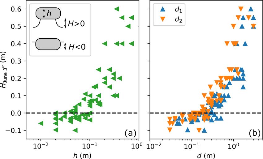
2622                                               M. Hénot et al.: Formation of glacier tables caused by differential ice melting

where λ is the thermal conductivity of granite (measured in a          small (−20 to 3 W m−2 ). The total turbulent flux QiH + QiE
previous work – Hénot et al., 2021 – as λ = 2.8 W m−1 K−1 ,            strongly differs between periods A and B. It decreases from
which is in agreement with the literature; Cho et al., 2009)           120 W m−2 (which represents 50 % of the total flux) in pe-
and d1D is a length scale for the conduction process in the            riod A to 25 W m−2 (10 % of the total flux) in period B.
rock. It was postulated and verified experimentally (see Fig. 5        This is due to the drastic difference in mean wind speed,
of Hénot et al., 2021) that this length could be estimated by          from 6.5 m s−1 during period A to 1.0 m s−1 during period
d1D = ηVrock /Aext = ηh/(1+4β), where Vrock is the volume              B, which explains the difference in the ice ablation rate (of
of the rock and η = 2.5 is a numerical prefactor adjusted              the order of 8 cm d−1 in period A and 5.5 cm d−1 in period
from the lab experiments. This expression justifies the def-           B).
inition of deff .
   From Eqs. (6) and (7) and using the measured meteoro-               4.2   Table formation
logical data (8(t), QLW atm ↓ (t), ua (t), Ta (t) and qa (t)) as
input, the rock surface temperature Trock (t) can be computed          Rocks 1 and 2 formed glacier tables over the course of ap-
at each time t by solving numerically non-linear Eq. (6).              proximately a week (see Fig. 4a and b), after which they fell
The flux Qrock→ice (t) reaching the ice can then be computed.          off the ice pedestal. Rock 3 was initially sitting on an ice
When positive, this leads to ice melting under the rock, low-          foot, which grew bigger, while rock 4, although exhibiting
ering the altitude of the bottom of the rock zrock :                   dimensions close to those of rock 2 went down almost at the
                                                                       same rate as the bare-ice surface and did not form any sig-
                               Zt                                      nificant glacier table (see the Supplement for pictures). The
zrock (t) − zice (0) = −Lfus        Qrock→ice (t)dt.            (8)    integration of the flux given by the model is shown in solid
                               0                                       lines in Fig. 4a and b. The best agreement with the observed
                                                                       data was obtained for a value of the adjustable parameter
The height of the ice foot supporting the rock is H (t) =              QLW env ↓ = 340 W m−2 . This corresponds to the long-wave
zrock (t) − zice (t). The time origin corresponds to the rock ly-      flux emitted by a surface with emissivity 1 at a temperature
ing at the surface of the ice (H (t = 0) = 0). Note that at this       278.3 K, which seems reasonable as the physical meaning of
stage, there are two adjustable parameters in the table for-           this quantity is the mean temperature of the environment seen
mation model: QLW env ↓ and z0 rock (αrock and η are taken             by the sides of the rocks (ice surface, others rocks and terrain
from the literature). However, the roughness size z0 in the            surrounding the glacier). The agreement between the mea-
turbulent coefficient is not clearly defined (Hock, 2005), but         surements and the model prediction is overall good for rocks
the resulting model is not very sensitive to its value. Thus in        1 to 3. The model overestimates slightly the ability to form a
the following, z0 rock will be taken as equal to that of the ice       table of rock 4, but the error (integrated over 6 d) stays under
z0 ice .                                                               3 cm for total ice ablation of 37 cm. Figure 6 shows the mea-
                                                                       sured temperature of the top surface of rock 4 (solid line) as
4     Results                                                          well as the value of Trock (t) predicted by the model. The two
                                                                       curves qualitatively display the same behaviour. The mean
4.1    Ice melting                                                     temperature is slightly overestimated by the model on aver-
                                                                       age (by 2 ◦ C), but the typical minimum (0–3 ◦ C) and maxi-
The dashed black lines in Fig. 4a and b correspond to the              mum (22–24 ◦ C) daily temperature remain close.
model described in Sect. 3.1 with parameters αice = 0.30 and              Figure 5 shows for each rock (in colour) the surface- and
z0 = 0.34 mm adjusted on the concatenated data of periods A            time-averaged radiative and turbulent flux computed from the
and B (see the Supplement for a discussion on the sensitiv-            model as well as the resulting heat flux transmitted to the
ity). The agreement between the model and the field mea-               ice underneath. The short-wave flux received on the top sur-
surements is good: the error on zice (t) stays below 3 cm (ex-         face of the rocks is 17 % higher than the one received by
cept at the end of period A when the movement of the camera            the ice due to the difference in albedo. However the net long-
increases the uncertainty in the measurements). The value of           wave and turbulent fluxes are significantly reduced due to the
the adjusted ice albedo corresponds to what is reported in             fact that on average the rocks’ surface temperature hTrock i
the literature for aged surface glacier ice, at the beginning          are higher than Tice . For rocks 1 to 4, the averaged surface
of summer (Brock et al., 2000). The value of the roughness             temperatures predicted were 8.2, 6.3, 13.0 and 7.2 ◦ C respec-
length z0 also falls in the range previously reported (10−4 –          tively. The turbulent flux reduction is more important during
10−2 m) (Brock et al., 2006; Conway and Cullen, 2013). Fig-            period A than during period B due to the higher mean wind
ure 5 shows (in white) the time-averaged values of QiSW ,              speed. Note that this effect is geometrically amplified (by a
QiLW and QiH , QiE as well as the total flux reaching the ice          factor 1 + 4β) as these negative fluxes are integrated over the
surface, Qopen env→ice , for both time periods. The short-wave         external surface of the rocks, which is larger than the base
flux varies weakly between periods A and B (from 150 to                surface in contact with ice (this is especially true for rock 4,
200 W m−2 ), and the net long-wave flux is comparatively               which has the largest aspect ratio). For all the rocks studied,

The Cryosphere, 16, 2617–2628, 2022                                                       https://doi.org/10.5194/tc-16-2617-2022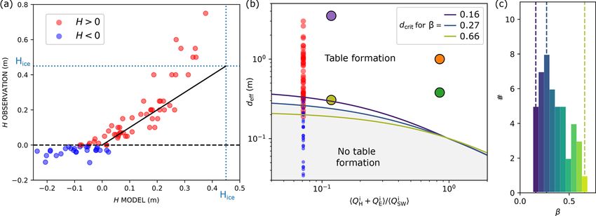
M. Hénot et al.: Formation of glacier tables caused by differential ice melting                                                           2623

Figure 5. (a) Schematics of the heat fluxes considered in the models for the ice surface melting (left) and glacier table formation. The colours
denote the surfaces on which the fluxes are received. (b, c) Distribution of the heat fluxes averaged over the duration of observation as
predicted by the time-resolved model for the ice surface (white) and for the four rocks studied (coloured).

Figure 6. Temperature Trock of the top surface of rock 4 measured using a thermocouple (light green) and predicted by the model using the
meteorological data of period B (dark line). The date format is year-month-day.

the predicted flux causing ice to melt under the rocks was on             solid lines in Fig. 7a correspond to linear adjustments. The
average reduced compared to the flux received by the ice sur-             deduced slopes hH /Hice i are plotted for each rock in Fig. 7b
face (from −15 % for rock 4 to −88 % for rock 3), leading                 as a function of their thickness h (markers). The value pre-
to the formation of tables. Note that this amplification effect           dicted by the model is plotted in the same figure for periods
can also, depending of the shape and size of the rocks, have              A (dashed lines) and B (solid lines) for the values of β cor-
the opposite consequence of causing a rock to sink into the               responding to the four rocks as a function of the thickness of
ice surface, as will be shown in Sect. 5.2.                               the rock. Moving along a line thus corresponds to a change in
    Figure 7a shows, for each rock, the height of the ice foot,           scale but not in shape of the rocks. The dimensionless growth
H (t) = zrock (t) − zice (t), as a function of the ablated ice            rates of the tables are accurately predicted by the model. It is
thickness, Hice (t) = zice (t) − zice (0). On average these quan-         visible that independently of the rock shape and time period,
tities appear to be proportional. The slope corresponds to a              a small enough rock would not form a table and instead sink
dimensionless growth rate of the glacier table, denoted as                into the ice surface (hH /Hice i < 0).
hH /Hice i: a unity slope would correspond to no melt under
the rock (the ice foot height would then correspond exactly               4.3    Analysis of the 80 glacier tables field
to the ablated ice thickness); conversely a zero slope would
correspond to a rock descending at the same rate as the ice               In Fig. 3, showing the height of the ice structure formed by
surface around it and thus never forming a glacier table. The             80 rocks 8 d after the melt of the snow layer, is it visible that

https://doi.org/10.5194/tc-16-2617-2022                                                           The Cryosphere, 16, 2617–2628, 2022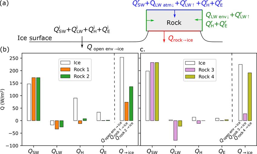
2624                                             M. Hénot et al.: Formation of glacier tables caused by differential ice melting

                                                                       than what is taken into account in the model. It is thus cooler,
                                                                       and its (negative) dimensionless growth rate is smaller (in ab-
                                                                       solute terms) than that given by the model, as observed. The
                                                                       rocks that have formed glacier tables (H > 0) are shown in
                                                                       red. The threshold between rocks forming or not forming a
                                                                       table (the point (0, 0) in the graph) is well predicted by the
                                                                       model. For the smaller structures (H < 0.3 m), the height of
                                                                       the ice foot is also well predicted (with an error smaller than
                                                                       5 cm). Note that this required no new adjustable parameter
                                                                       and this prediction is the result of a model integrated over 8 d
                                                                       in a time period different from A and B, during which the pa-
                                                                       rameters of the model were adjusted. For ice feet taller than
                                                                       0.3 m, however, the prediction of the model is not good. For
                                                                       some H > Hice , and the assumption H26 May = 0 is thus ob-
                                                                       viously not valid. We infer that larger rocks emerged from the
                                                                       snow layer before 26 May and started to form a table earlier.

                                                                       5     Discussion
Figure 7. (a) Evolution of the height H of the ice foot under rocks
1–4 as a function of the ablated ice thickness Hice . The coloured     5.1    Critical diameter
lines correspond to linear adjustments of the data. The solid black
line has a slope of 1. (b) The mean ratio of the height H of the ice   The critical diameter, corresponding to the transition be-
foot under a rock and of the total ablated ice thickness Hice since    tween the two regimes described in the previous section (the
the beginning of the table formation, as a function of the thickness   rock sinks into the ice or forms a table), is denoted as dcrit . We
h of the rock. The markers correspond to the slopes of (a) for each    chose to consider a critical width instead of a critical thick-
rock. The lines correspond to the application of the model for the     ness as the transition seems sharper when considering this
meteorological values measured in period A (dashed lines) and B        quantity in Fig. 3. This is reminiscent of the results obtained
(solid lines) and the aspect ratio β of each rock given in Table 1.    in a controlled environment in the absence of solar radiation,
                                                                       for which the transition occurred for a critical diameter of
                                                                       the cylinders, independently of their aspect ratio (Hénot et
a critical size exists (4–10 cm in thickness and 9–13 cm in            al., 2021).
width) above which rocks tend to form glacier tables. The                 From our model, given a set of meteorological data
larger the rock, the greater its ability to protect the ice un-        and an aspect ratio β, a critical width dcrit can be com-
derneath from melting and, assuming all tables started their           puted. In the following, unlike what has been done un-
formation at the same time, the higher the ice foot. Below             til now, typical time-averaged meteorological data (h8i =
this critical size, however, the rocks have a tendency to sink         210 W m−2 , hQLW atm ↓ i = 315 W m−2 , hTa i = 7 ◦ C, hqa i =
into the ice surface. Having successfully modelled the evolu-          0.0058 kg kg−1 and hua i ranging from 0 to 20 m s−1 ) will be
tion of the four larger glacier tables, the model presented in         used as inputs (we have checked that this pre-averaging of
Sect. 3.2 can be applied to the data obtained on a given day           the input data affects the output of the model by less than
for a field comprising 80 rocks.                                       a few percent). Figure 8b shows a diagram of the ability of
   The snow layer covering that part of the glacier finished           a rock to form a table as a function of its effective width
melting on 26 May, leaving the ice exposed. The meteo-                 deff (which in practice can be replaced by the mean width)
rological data of the time period C (from 26 May until                 and the ratio hQiH + QiE i/hQiSW i, which is a quantity propor-
3 June), alongside the previously adjusted parameters αice             tional to hua i and whose relevance will be discussed in the
and z0 , allow us to compute the thickness of ablated ice              next paragraph. The four monitored rocks as well as the field
Hice = 0.45 ± 0.05 m during this period (see Fig. S5 in the            data from the 80 rocks found in the 800 m2 field are plotted in
Supplement). The observed values of H are plotted in Fig. 8a           this diagram. The distribution of aspect ratio β of rocks (46 of
as a function of the ones predicted by the model for each              them) close to the transition (defined by |H | < 0.2 m) is plot-
rock, assuming that the structure formation started on 26 May          ted in Fig. 8c. The bounding values (β = 0.16 and β = 0.66)
(H26 May = 0). The rocks that have sunk into the ice surface           as well as the value corresponding to the maximum of the dis-
(H < 0) are shown in blue. For those, the prediction of the            tribution (β = 0.27) are used to plot, in Fig. 8b, the values of
model is, as expected, not accurate. Indeed, a rock that has           dcrit predicted by the model. This threshold, which depends
penetrated into the ice has a greater contact surface area with        slightly on β, shows a good agreement with the transition
the ice and a smaller external surface open to the atmosphere          visible in the field data. This diagram illustrates the sensitiv-

The Cryosphere, 16, 2617–2628, 2022                                                        https://doi.org/10.5194/tc-16-2617-2022
M. Hénot et al.: Formation of glacier tables caused by differential ice melting 2625
Figure 8. (a) Observation versus model for the distance H between the bottom of rocks and the ice surface for the data measured on 3 June
2021 (see Fig. 3). The data are represented in red if a table is observed (H > 0) and in blue otherwise. The solid black line has a slope of 1,
and the dotted lines correspond to the ablated ice thickness Hice since the melting of the snow layer (see the Supplement). (b) Diagram of
the ability of a rock to form a table as a function of its typical width deff and the ratio hQiH + QiE i/hQiSW i. The solid lines correspond, for
three values of the aspect ratio β, to the delimitation predicted by the model with averaged meteorological data, between a rock forming a
table and a rock sinking into the ice surface. The small circles correspond to the data of (a) with the same colour code. The larger circles
correspond to rocks 1–4. (c) Distribution of the aspect ratio β of the rocks close to the transition between the two regimes (|H | < 0.2 m). The
vertical dashed lines correspond to the limits plotted in (b) with the same colour code.
ity of the glacier table formation to the meteorological con- The ratio hQiH + QiE i/hQiSW i used on the abscissa in Fig. 8b
ditions and especially the mean wind speed: deff is divided demonstrates this effect. When this ratio is small (< 0.1), the
by 2 between time periods A and B. structure formation is controlled by the long-wave emission
of the rock, while a large value (> 1) would correspond to a
5.2 Physical discussion regime dominated by the effect of sensible flux. Note that at
this point, a 1D model with d1D = h and no geometrical am-
A rock forms a glacier table when the heat flux reaching plification would have achieved the same result. However,
the ice underneath is reduced compared to that received by the 3D structure has its importance: the heat transfer with the
the bare-ice surface around it. If, on the contrary, this heat environment (short-wave and turbulent) that cools the rock is
flux is amplified, the rock will sink into the ice surface. De- exchanged on a surface area with is much larger than the base
pending on the rock size, both phenomena are observed on area of a rock. In our model we considered the total exter-
temperate glaciers. During summer, the main source of heat nal surface of the rock, which is larger by a factor of 1 + 4β
flux causing the ice to melt is the short-wave radiation com- typically of the order of 2–3 than Abase . As detailed in the
ing from the sun. Due to the lower albedo of the rock, this Supplement, a 1D model would, in order to verify Eq. (6),
flux is slightly amplified compared to what is received by significantly overestimate Trock (by 150 ◦ C during sunlight
a similar area of bare ice and thus does not directly favour for rock 3, which is not a physically acceptable value). This
the formation of glacier tables. However this induces a heat 3D effect also explains the influence of the rock shape on its
flux across the thickness of the rock that elevates its sur- ability to form a table.
face temperature Trock (the bottom surface staying at Tice ) The formation of glacier tables in the natural environment
and strongly affects the net infrared radiation and turbulent of a temperate glacier results from a more complex energy
fluxes. As can be seen in Fig. 5, the sign of the sensible balance than the idealized lab-controlled study conducted
flux can even change (if Trock > Ta > Tice , the wind warms previously (Hénot et al., 2021) while the main physical in-
the ice surface but cools the rock) and induces a negative gredient stays the same: the greater temperature of the rock
net short-wave flux (the rock flux lost being proportional to surface, compared to the ice, reduces the incoming heat flux
4 ). At the end, if the rock is large enough (so that its sur-
Trock and thus the melt rate under the rock. In the absence of so-
face temperature can rise enough), all these combined effects lar radiation, the threshold controlling the ability of a rock to
lead to the formation of a glacier table. As illustrated by the form a table was determined by a trade-off between this ef-
difference between periods A and B, the wind intensity can fect and a geometrical amplification effect: a rock can act as
vary significantly at the surface of the glacier. The sensible a fin in amplifying the incoming heat flux, leading to a higher
flux being one motor of glacier table formation (with emit- melt rate under the rock than for bare ice. While this effect
ted long-wave radiation), this affects the critical size dcrit . also plays a role in natural conditions, the threshold is also
https://doi.org/10.5194/tc-16-2617-2022 The Cryosphere, 16, 2617–2628, 20222626 M. Hénot et al.: Formation of glacier tables caused by differential ice melting
significantly affected by the direct solar radiation that has dimensionless growth rate of the ice foot hH /Hice i that char-
two opposite effects: on the one hand, due to lower albedo, a acterize the ability of a rock to form a table: the rock thick-
higher flux is received by a rock than a bare-ice surface, but, ness h; its aspect ratio β; and the ratio hQiH + QiE i/hQiSW i,
on the other hand, the temperature gradient induced by the which depends on the meteorological conditions. When this
solar flux across a rock elevates its temperature, enhancing ratio is higher than ≈ 0.1 (i.e. in windy periods), the turbu-
the cooling effect due to turbulent and long-wave flux. The lent heat exchange lowers the critical diameter dcrit (by up to
first effect dominates for small rocks, while the latter domi- 50 %), which facilitates glacier table formation. We did not
nates for larger rocks. consider in this study the lateral melting of the ice pedestal
While the heat transfer across the rock controls the forma- and the end of life of the structures, but this could be the
tion dynamics, the end of life of glacier tables and in particu- subject of future work.
lar the maximum height reached by ice feet will likely result
from lateral melting of the ice column. This process is ex-
pected to be affected by the rock shape and size that would Code availability. The graphical user interface (GUI) devel-
prevent radiative melting due to shading effects, leaving only oped to extract the data from the raw images is available
turbulent flux and long-wave balance. Note also that when at https://doi.org/10.5281/zenodo.6683570 (Hénot, 2022). Python
the ice pedestal becomes very slender, a heavy rock could script files used to generate the figures are available upon request
to the corresponding author.
also cause the ice column to creep.
Data availability. The S2M data used in this work provided by
6 Conclusions Météo-France CNRS, CNRM Centre d’Etudes de la Neige, through
AERIS, are available at https://doi.org/10.25326/37#v2020.2 (Ver-
We studied the formation of four glacier tables over the nay et al., 2022b). All other data used in this work are available
course of a week, and we measured the characteristics of 80 upon request to the corresponding author for non-commercial re-
glacier tables on the Mer de Glace (Alps). We developed a search use.
simple model taking into account the infrared and solar ra-
diation and turbulent heat flux received by a rock and by the
glacier ice surface using local meteorological data, allowing Supplement. The supplement related to this article is available on-
us to quantitatively reproduce the glacier table formation dy- line at: https://doi.org/10.5194/tc-16-2617-2022-supplement.
namics and to identify the physical effects at its origin. The
table formation is controlled by the ice melting under the
rocks, and the ice foot growth rate is proportional to the ice Author contributions. MH, VL, JV, NP and NT conceived the study
ablation rate at the glacier surface. The size of the rocks is a and performed the fieldwork. MH performed the data analysis, de-
determinant factor governing table formation: the bigger the veloped the model and drafted the manuscript. All authors con-
tributed to the data interpretation, discussion of the results and writ-
rock, the higher and faster the ice foot supporting it will grow.
ing of the manuscript.
Under a critical size, rocks show the opposite behaviour of
sinking into the ice surface. The ability of a rock to form a
table is controlled by the balance between two opposing ef- Competing interests. The contact author has declared that neither
fects: a thermal insulation effect, which depends strongly on they nor their co-authors have any competing interests.
the rock size, and a geometrical amplification effect linked
to the fact that the external surface on which the rock re-
ceives an external heat flux is larger than its contact area with Disclaimer. Publisher’s note: Copernicus Publications remains
the ice. This second effect becomes dominant only for rocks neutral with regard to jurisdictional claims in published maps and
smaller than a few tens of centimetres. The insulation effect institutional affiliations.
originates from the warmer temperature of the rock surface
compared to the ice, which reduces, even sometimes chang-
ing the sign of, the net long-wave and turbulent flux, ulti- Acknowledgements. The authors acknowledge technical sup-
mately reducing the heat available for ice melting under the port and useful scientific discussion with Marine Vicet and
rock. While a rock receives a slightly larger net short-wave Thierry Dauxois. The S2M data are provided by Météo-France
flux (the main source of heat at the glacier surface) than ice CNRS, CNRM Centre d’Etudes de la Neige, through AERIS.
because of the difference in albedo, this effect is too weak
to compensate for the insulation effect for large rocks. The
solar radiation, by inducing a strong thermal gradient across Financial support. This research has been supported by the Fédéra-
tion de Recherche André-Marie Ampère and Laboratoire de
the thickness of the rock, raises the rock surface tempera-
Physique at ENS de Lyon.
ture, which also contributes to the insulation effect. To sum-
marize, we identified three main parameters controlling the
The Cryosphere, 16, 2617–2628, 2022 https://doi.org/10.5194/tc-16-2617-2022M. Hénot et al.: Formation of glacier tables caused by differential ice melting 2627
Review statement. This paper was edited by Chris R. Stokes and Claudin, P., Durán, O., and Andreotti, B.: Dissolution insta-
reviewed by Adrien Gilbert and two anonymous referees. bility and roughening transition, J. Fluid Mech., 832, R2,
https://doi.org/10.1017/jfm.2017.711, 2017.
Cohen, C., Berhanu, M., Derr, J., and du Pont, S. C.: Erosion pat-
terns on dissolving and melting bodies, Physical Review Flu-
References ids, 1, 050508, https://doi.org/10.1103/PhysRevFluids.1.050508,
2016.
Agassiz, L.: Études sur les glaciers, Gent & Gassman, Neuchâ- Cohen, C., Berhanu, M., Derr, J., and Du Pont, S. C.:
tel, LCCN (Librairy of congress catalog), https://lccn.loc.gov/ Buoyancy-driven dissolution of inclined blocks: Erosion rate
12008544 (last access: 23 June 2022), 1840. and pattern formation, Physical Review Fluids, 5, 053802,
Bergeron, V., Berger, C., and Betterton, M. D.: Controlled Irra- https://doi.org/10.1103/PhysRevFluids.5.053802, 2020.
diative Formation of Penitentes, Phys. Rev. Lett., 96, 098502, Collier, E., Nicholson, L. I., Brock, B. W., Maussion, F., Essery,
https://doi.org/10.1103/physrevlett.96.098502, 2006. R., and Bush, A. B. G.: Representing moisture fluxes and phase
Betterton, M. D.: Theory of structure formation in snowfields mo- changes in glacier debris cover using a reservoir approach, The
tivated by penitentes, suncups, and dirt cones, Phys. Rev. E, 63, Cryosphere, 8, 1429–1444, https://doi.org/10.5194/tc-8-1429-
056129, https://doi.org/10.1103/PhysRevE.63.056129, 2001. 2014, 2014.
Bintanja, R., Reijmer, C. H., and Hulscher, S. J. M. Conway, J. and Cullen, N.: Constraining turbulent heat
H.: Detailed observations of the rippled surface of flux parameterization over a temperate maritime
Antarctic blue-ice areas, J. Glaciol., 47, 387–396, glacier in New Zealand, Ann. Glaciol., 54, 41–51,
https://doi.org/10.3189/172756501781832106, 2001. https://doi.org/10.3189/2013AoG63A604, 2013.
Bordiec, M., Carpy, S., Bourgeois, O., Herny, C., Massé, M., Drewry, D. J.: A Quantitative Assessment of
Perret, L., Claudin, P., Pochat, S., and Douté, S.: Sublima- Dirt-Cone Dynamics, J. Glaciol., 11, 431–446,
tion waves: Geomorphic markers of interactions between icy https://doi.org/10.3189/S0022143000022383, 1972.
planetary surfaces and winds, Earth-Sci. Rev., 211, 103350, Evatt, G., Mayer, C., Mallinson, A., Abrahams, I., Heil, M., and
https://doi.org/10.1016/j.earscirev.2020.103350, 2020. Nicholson, L.: The secret life of ice sails, J. Glaciol., 63, 1049–
Bouillette, E.: Une Superbe Table des Glaciers, L’Astronomie, 47, 1062, https://doi.org/10.1017/jog.2017.72, 2017.
201–202, 1933. Evatt, G. W., Abrahams, I. D., Heil, M., Mayer, C., Kingslake,
Bouillette, E.: La fin d’une table des glaciers, L’Astronomie, 48, J., Mitchell, S. L., Fowler, A. C., and Clark, C. D.: Glacial
89–91, 1934. melt under a porous debris layer, J. Glaciol., 61, 825–836,
Brock, B. W., Willis, I. C., and Sharp, M. J.: Measure- https://doi.org/10.3189/2015JoG14J235, 2015.
ment and parameterization of albedo variations at Haut Fitzpatrick, N., Radić, V., and Menounos, B.: Surface Energy Bal-
Glacier d’Arolla, Switzerland, J. Glaciol., 46, 675–688, ance Closure and Turbulent Flux Parameterization on a Mid-
https://doi.org/10.3189/172756500781832675, 2000. Latitude Mountain Glacier, Purcell Mountains, Canada, Front.
Brock, B. W., Willis, I. C., and Sharp, M. J.: Measurement and Earth Sci., 5, 67, https://doi.org/10.3389/feart.2017.00067, 2017.
parameterization of aerodynamic roughness length variations at Fowler, A. C. and Mayer, C.: The formation of
Haut Glacier d’Arolla, Switzerland, J. Glaciol., 52, 281–297, ice sails, Geophys. Astro. Fluid, 111, 411–428,
https://doi.org/10.3189/172756506781828746, 2006. https://doi.org/10.1080/03091929.2017.1370092, 2017.
Bruthans, J., Soukup, J., Vaculikova, J., Filippi, M., Guérin, A., Derr, J., Du Pont, S. C., and Berhanu,
Schweigstillova, J., Mayo, A. L., Masin, D., Kletetschka, M.: Streamwise dissolution patterns created by a
G., and Rihosek, J.: Sandstone landforms shaped by negative flowing water film, Phys. Rev. Lett., 125, 194502,
feedback between stress and erosion, Nat. Geosci., 7, 597–601, https://doi.org/10.1103/PhysRevLett.125.194502, 2020.
https://doi.org/10.1038/ngeo2209, 2014. Hardy, B.: ITS-90 Formulations for Vapor Pressure, Frost point
Bushuk, M., Holland, D. M., Stanton, T. P., Stern, A., Temperature, Dew point Temperature, and Enhancement Factors
and Gray, C.: Ice scallops: a laboratory investigation of in the range −100 to +100 C”, Papers and Abstracts of the Third
the ice–water interface, J. Fluid Mech., 873, 942–976, International Symposium on Humidity and Moisture, Tedding-
https://doi.org/10.1017/jfm.2019.398, 2019. ton, London, England, April 1998, https://api.semanticscholar.
Carenzo, M., Pellicciotti, F., Mabillard, J., Reid, T., and Brock, B. org/CorpusID:98492826 (last access: 23 June 2022), 214–222,
W.: An enhanced temperature index model for debris-covered 1998.
glaciers accounting for thickness effect, Adv. Water Resour., Hénot, M.: Pointing interface, Zenodo [code],
94, 457–469, https://doi.org/10.1016/j.advwatres.2016.05.001, https://doi.org/10.5281/zenodo.6683570, 2022.
2016. Hénot, M., Plihon, N., and Taberlet, N.: Onset of
Cho, W., Kwon, S., and Choi, J.: The thermal conductivity for Glacier Tables, Phys. Rev. Lett., 127, 108501,
granite with various water contents, Eng. Geol., 107, 167–171, https://doi.org/10.1103/PhysRevLett.127.108501, 2021.
https://doi.org/10.1016/j.enggeo.2009.05.012, 2009. Hock, R.: Glacier melt: a review of processes and their modelling,
Claudin, P., Jarry, H., Vignoles, G., Plapp, M., and Andreotti, B.: Progress in Physical Geography: Earth and Environment, 29,
Physical processes causing the formation of penitentes, Phys. 362–391, https://doi.org/10.1191/0309133305pp453ra, 2005.
Rev. E, 92, 033015, https://doi.org/10.1103/physreve.92.033015, Huang, J. M., Tong, J., Shelley, M., and Ristroph, L.:
2015. Ultra-sharp pinnacles sculpted by natural convective dis-
https://doi.org/10.5194/tc-16-2617-2022 The Cryosphere, 16, 2617–2628, 20222628 M. Hénot et al.: Formation of glacier tables caused by differential ice melting solution, P. Natl. Acad. Sci. USA, 117, 23339–23344, Rhodes, J. J., Armstrong, R. L., and Warren, S. G.: https://doi.org/10.1073/pnas.2001524117, 2020. Mode of Formation of “Ablation Hollows” Controlled Huinink, H. P., Pel, L., and Kopinga, K.: Simulating the by Dirt Content of Snow, J. Glaciol., 33, 135–139, growth of tafoni, Earth Surf. Proc. Land., 29, 1225–1233, https://doi.org/10.3189/S0022143000008601, 1987. https://doi.org/10.1002/esp.1087, 2004. Smiraglia, C. and Diolaiuti, G.: Encyclopedia of Snow, Ice and Krenek, L. O.: The Formation of Dirt Cones on Mount Glaciers, Chap. Epiglacial Morphology, Springer, 262–267, Ruapehu, New Zealand, J. Glaciol., 3, 312–315, ISBN 978-90-481-2641-5, 2011. https://doi.org/10.3189/S0022143000023984, 1958. Swithinbank, C.: The origin of dirt cones on glaciers, J. Glaciol., 1, Lienhard, J. H.: A Heat Transfert Textbook, Phlogiston Press, 411– 461–465, https://doi.org/10.3189/S0022143000012880, 1950. 428, ISBN 9780486837352, 2019. Taberlet, N. and Plihon, N.: Sublimation-driven morphogenesis Mangold, N.: Ice sublimation as a geomorphic process: of Zen stones on ice surfaces, P. Natl. Acad. Sci. USA, 118, A planetary perspective, Geomorphology, 126, 1–17, e2109107118, https://doi.org/10.1073/pnas.2109107118, 2021. https://doi.org/10.1016/j.geomorph.2010.11.009, 2011. Turkington, A. V. and Paradise, T. R.: Sandstone weathering: a cen- Mashaal, N. M., Sallam, E. S., and Khater, T. M.: Mushroom rock, tury of research and innovation, Geomorphology, 67, 229–253, inselberg, and butte desert landforms (Gebel Qatrani, Egypt): https://doi.org/10.1016/j.geomorph.2004.09.028, 2005. evidence of wind erosion, Int. J. Earth Sci., 109, 1975–1976, Vernay, M., Lafaysse, M., Monteiro, D., Hagenmuller, P., Nheili, https://doi.org/10.1007/s00531-020-01883-z, 2020. R., Samacoïts, R., Verfaillie, D., and Morin, S.: The S2M mete- McIntyre, N. F.: Cryoconite hole thermodynamics, Can. J. Earth orological and snow cover reanalysis over the French mountain- Sci., 21, 152–156, https://doi.org/10.1139/e84-016, 1984. ous areas: description and evaluation (1958–2021), Earth Syst. Michalski, J., Reynolds, S., Sharp, T., and Christensen, P.: Sci. Data, 14, 1707–1733, https://doi.org/10.5194/essd-14-1707- Thermal infrared analysis of weathered granitic rock com- 2022, 2022a. positions in the Sacaton Mountains, Arizona: Implica- Vernay, M., Lafaysse, M., Hagenmuller, P., Nheili, R., Verfaillie, tions for petrologic classifications from thermal infrared D., and Morin, S.: The S2M meteorological and snow cover re- remote-sensing data, J. Geophys. Res.-Planet., 109, E03007, analysis in the French mountainous areas (1958–present), AERIS https://doi.org/10.1029/2003JE002197, 2004. [data set], https://doi.org/10.25326/37#v2020.2, 2022b. Mitchell, K. A. and Tiedje, T.: Growth and fluctuations of sun- Watson, R. D.: Spectral reflectance and photometric proper- cups on alpine snowpacks, J. Geophys. Res., 115, F04039, ties of selected rocks, Remote Sens. Environ., 2, 95–100, https://doi.org/10.1029/2010JF001724, 2010. https://doi.org/10.1016/0034-4257(71)90082-4, 1971. Moeller, R., Moeller, M., Kukla, P. A., and Schneider, C.: Im- Weady, S., Tong, J., Zidovska, A., and Ristroph, L.: pact of supraglacial deposits of tephra from Grímsvötn vol- Anomalous Convective Flows Carve Pinnacles and Scal- cano, Iceland, on glacier ablation, J. Glaciol., 62, 933–943, lops in Melting Ice, Phys. Rev. Lett., 128, 044502, https://doi.org/10.1017/jog.2016.82, 2016. https://doi.org/10.1103/PhysRevLett.128.044502, 2022. Nadeau, D. F., Brutsaert, W., Parlange, M., Bou-Zeid, E., Bar- Young, R. and Young, A.: Sandstone Landforms, Lecture Notes in renetxea, G., Couach, O., Boldi, M.-O., Selker, J. S., and Vetterli, Physics, Springer-Verlag, ISBN 9780387539461, https://books. M.: Estimation of urban sensible heat flux using a dense wire- google.fr/books?id=Da8rvwEACAAJ (last access: 1 June 2022), less network of observations, Environ. Fluid Mech., 9, 635–653, 1992. https://doi.org/10.1007/s10652-009-9150-7, 2009. Östrem, G.: Ice Melting under a Thin Layer of Moraine, and the Existence of Ice Cores in Moraine Ridges, Geogr. Ann., 41, 228– 230, http://www.jstor.org/stable/4626805, 1959. Reid, T. D. and Brock, B. W.: An energy-balance model for debris-covered glaciers including heat conduc- tion through the debris layer, J. Glaciol., 56, 903–916, https://doi.org/10.3189/002214310794457218, 2010. The Cryosphere, 16, 2617–2628, 2022 https://doi.org/10.5194/tc-16-2617-2022
You can also read