Favoritism and Firms: Micro Evidence and Macro Implications - ZEW
←
→
Page content transcription
If your browser does not render page correctly, please read the page content below
// NO.21-031 | 06/2021

DISCUSSION
     PAPER
  / / Z A R E H A S AT R Y A N , T H U S H Y A N T H A N B A S K A R A N ,
              C A R LO B I R K H O L Z, A N D DAV I D G O MTSYA N

Favoritism and Firms:
Micro Evidence and Macro
Implications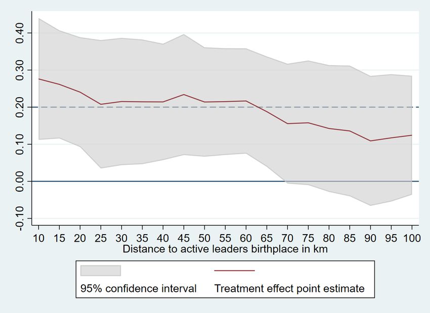
Favoritism and Firms:
  Micro Evidence and Macro Implications

                 Zareh Asatryan∗†                Thushyanthan Baskaran∗‡

                  Carlo Birkholz∗§                     David Gomtsyan∗¶

                                 First Version: February 2021

                                    This Version: June 2021

                                               Abstract
       We study the economic implications of regional favoritism, a form of distributive politics
       that channels resources geographically within countries. We utilize enterprise surveys
       spanning many low and middle income countries, and exploit transitions of national
       political leaders for identification. We document strong evidence for regional favoritism
       among firms located close to current leader’s birthplace, but not in other regions, nor in
       home regions before a leader takes office. Firms in favored regions become substantially
       larger in terms of sales and employment. They also increase their sales per worker, pay
       higher wages, and have higher measured total factor productivity. Several mechanisms
       suggests that leaders divert public resources into their home regions by generating higher
       demand for firms operating in the non-tradable sector. A simple structural model of
       resource misallocation that is calibrated to match our empirical estimates implies that
       favoritism generates aggregate output losses of 0.5% annually.

JEL codes: D22, D72, O43, R11.
Keywords: Regional favoritism, firm performance, enterprise surveys, resource misallocation.

   ∗
     We thank Andreas Fuchs, Francesco Amodio, Leonardo Giuffrida, Patrick Hufschmidt, as well as seminar
participants in Mannheim and Frankfurt. We also thank Nikoloz Chkheidze for excellent research assistance,
and Joshua Wimpey from the World Bank Group for sharing and helping us use the enterprise data. We
acknowledge financial support from the German Research Foundation (DFG) within the Project “Regional
Favoritism and Development” (Grant no. 423358188 / BA 496716-1). The usual disclaimer applies.
†
  ZEW Mannheim and CESifo, zareh.asatryan@zew.de.
‡
  University of Siegen, thushyanthan.baskaran@gmail.com.
§
  ZEW Mannheim and University of Mannheim, carlo.birkholz@zew.de.
¶
  IOS Regensburg, dgomtsyan@gmail.com.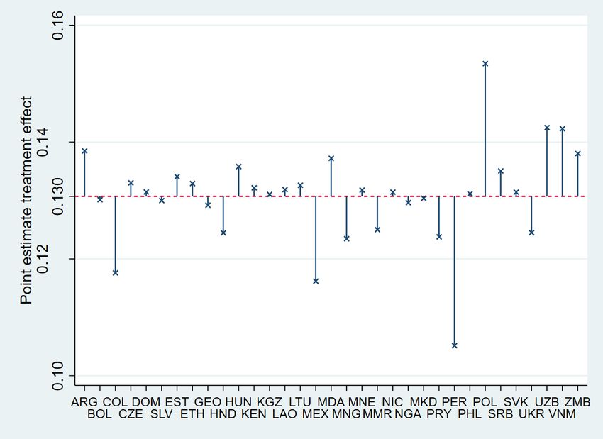
1     Introduction

Regional favoritism - that is, the geographic redistribution of resources within countries based
on preferential political treatment - is a large phenomenon observed in many parts of the
world (Hodler and Raschky 2014). Economists have long studied the question of whether
and how distributive politics - including political and regional favoritism - lead to distortionary
economic policies (Golden and Min 2013). The literature has hypothesized that lower income
and less democratic countries chronically suffer from various types of distortive policies, which
presumably widen the income gap between high and low income countries.
     Our aim is to shed light on whether regional favoritism should be viewed as a policy
failure that necessarily leads to more divergent economic outcomes, or whether it can be
thought of as a type of industrial policy that may potentially improve economic development.
To answer this question, we examine whether regional favoritism impacts firm performance.
We remain agnostic regarding the normative mechanisms of favoritism at play. On the one
hand, favoritism is likely to diminish welfare if leaders misallocate the factors of production to
unproductive firms and regions, for example, due to political connections and corrupt motives.
On the other hand, favoritism can improve welfare if leaders can provide at least a selected
set of firms and regions the push necessary to grow, become more productive and enter
international markets.
     To study this trade-off, we employ survey data from a maximum of 125,000 enterprises
in 120 low and middle income countries and utilize transitions of national political leaders for
identification (see the geography of the firms and leaders in Figure 1). Our first contribution
is to document the existence of strong regional favoritism in firm outcomes. Firms located
in the home regions of current political leaders are larger in terms of their sales and the
number of employees than firms located in other regions. Exploiting information on the
exact geo-location of firms, we show that these effects of favoritism are strongest in a 10
km radius around a leader’s birthplace, and that the effects diminish by distance. In our
baseline specification, we find that favored firms located within about a 50 km radius of the

                                                2
leader’s birthplace have 22% higher sales and 13% more employees compared to control firms.
For an average firm, these effects translate into $1.5 million more in sales and 10 additional
employees. Our placebo analysis does not find evidence for pre-trends, suggesting that the
causality likely runs from leader changes to firm outcomes.
We then exploit the richness of our enterprise survey data and study the mechanisms
that lead to such outcomes. We find that firms located in favored regions are not only larger
in size, but that they also produce more output per worker, pay higher wages, and have
higher total factor productivity compared to other firms. This evidence is consistent with the
interpretation that regional favoritism may be an efficient policy. However, several additional
pieces of evidence speak against this hypothesis. First, our results indicate that the effects
are driven by the non-tradable sector. In the literature, episodes of rapid expansion of the
non-tradable sector, relative to the tradable, are associated with the inflows of funds. These
may be driven by natural resource booms, remittances, or borrowing, all of which increase
the demand for non-tradable goods (see van der Ploeg 2011 for a comprehensive survey of
the literature). By contrast, general productivity improvements should lead to more balanced
growth in the two sectors. Second, and relatedly, we do not find evidence for higher export
rates among manufacturing firms. Third, we find that the expansion of firms is partly fueled
by direct government transfers in the form of more public procurement contracts. Fourth, the
effects on firms are temporary, such that they cease almost immediately after a leader leaves
office. Fifth, firms located in favored regions do not perceive any improvements in the business
environment - if anything, they express an unfavorable view of the available infrastructure and
quality of the workforce. Overall, these results are consistent with the interpretation that
leaders divert public resources to their home regions, thus generating higher demand for
output produced by firms operating in the non-tradable sector. This redistribution comes at
the cost of other regions and is thus indicative of misallocation of resources.
As a third and final step, we set up a simple misallocation model in the spirit of Restuccia
and Rogerson (2008). We use the model to quantify the aggregate implications of regional
favoritism. We consider an economy with two regions and two sectors, where firms face
3wedges driven by favoritism. We calibrate the model to match the moments that we estimate
empirically. Our counterfactual exercise shows that in an economy with spatial wedges driven
by favoritism, output is 0.5% lower compared to a distortion free economy. The intuition
behind this result is that the redistribution between regions increases incomes in the home
region and thus demand. The demand for non-tradable goods can be satisfied only by the
local production, while the demand for tradable goods can also be met through imports from
the other region. Therefore, factors of production will reallocate towards the non-tradable
sector in the leaders’ home region and the tradable sector in the non-home region. A higher
concentration of labor in sectors decreases the marginal productivity of firms and results in
aggregate losses.
This paper is related to two strands of literature. First, we contribute to the evolving
literature on regional favoritism. i Miquel et al. (2007) were one of the first to lay down the
theoretical framework for favoritism, while Hodler and Raschky (2014) were one of the first
to document evidence for it. In particular, Hodler and Raschky (2014) use satellite data from
across the globe and find a higher intensity of nighttime light in the birthplaces of the countries’
political leaders compared to other regions within countries. In a closely coupled strand of
literature, de Luca et al. (2018), Dickens (2018) observe higher nighttime light intensity in
political leaders’ ethnic homelands. Relatedly, Amodio et al. (2019), Asatryan et al. (2021),
Franck and Rainer (2012), Kramon and Posner (2016) find evidence for improved human
capital outcomes (e.g. in health, education and labor-markets) among individuals belonging
to either the same ethnicity or coming from the same region as those holding political power.
Several papers extend this work on ethno-regional favoritism to various sets of policies, such as
road building in Kenyan districts (Burgess et al. 2015) and Sub-Saharan Africa more broadly
(Bandyopadhyay and Green 2019), infrastructure projects in Vietnam (Do et al. 2017),
school construction in Benin (André et al. 2018), enforcement of audits (Chu et al. 2021)
and taxes (Chen et al. 2019) in China, mining activities in Africa (Asatryan et al. 2021),
and the allocation of foreign aid in Africa (Anaxagorou et al. 2020, Dreher et al. 2019),
among others.
4Second, our paper relates to an important strand in the literature on how the misallocation
of factors of production leads to substantial differences in aggregate total factor productivity.
This literature goes back to Hsieh and Klenow (2009, 2010), Restuccia and Rogerson (2008),
and is surveyed by Hopenhayn (2014), Restuccia and Rogerson (2017). In this context several
studies have used the enterprise survey data to estimate aggregate output losses caused by
various institutional frictions (Besley and Mueller 2018, Ranasinghe 2017). Our contribution
is to highlight a new source of misallocation that is driven by regional favoritism and which
is caused by the endogenous concentration of production factors in opposite sectors in each
region. Several related papers study efficiency losses caused by policy distortions in spatial
contexts. Brandt et al. (2013) study China’s economy in a model with multiple provinces and
two types of firms (private and state-owned). Desmet and Rossi-Hansberg (2013) introduce
labor wedges to a model with cities to asses efficiency losses in the US and China. Fajgel-
baum et al. (2018) use an economic geography model to estimate welfare losses caused by
heterogeneity in tax systems across US states.
2 Empirical design
2.1 Data
Firms Our firm-level data are drawn from the World Bank Enterprise Surveys, which have
been administered using a global methodology since 2006. The full sample of these surveys
spans over 140 countries; however only 98 countries have been surveyed more than once. In
these countries, survey waves are typically carried out in two to five year intervals, leading on
average to 2.5 survey waves per country. Surveys cover the non-agricultural formal private
sector, thus excluding firms which are fully government owned, are informal, or are classified
as agricultural firms according to ISIC revision 3.1. Firms are drawn by stratified random
sampling, with stratification performed based on firm size, geographic location within the
country, and sector of activity. Furthermore, firms are required to have five or more employees.
5The number of firms sampled in a given country varies with the size of its economy. Large,
medium and small economies host, respectively, 1200-1800, 360 and 150 interviews.1
The enterprise surveys contain information on general firm characteristics such as their
age, ownership structure, and sector, as well as indicators of their performance in terms of
sales, employment, and input factors. In addition, firms are asked about their management
practices, relations to the government, crime and corruption, and the business environment.
These latter aspects allow us to study favoritism’s effects and channels in greater detail.
For the main part of our empirical analysis we consider the sub-sample of surveys carried
out since 2009, as they provide us with geocoded data on the location of firms.2 In additional
specifications we use the general sample, and we identify the location of firms according to
administrative regions. However, there are occasionally changes in the definition of regions
between survey waves. Therefore, we give priority to the smaller sub-sample of geocoded
data to achieve greater precision and to perform detailed spatial analysis, while we rely on the
larger sample to test the robustness of our baseline findings.
In total there are around 100,000 and 150,000 enterprise surveys carried out in the
geocoded and regional samples, respectively. However, the key variables we use have missing
values to a varying degree. Additionally, to alleviate bias in our estimates from outliers, we
exclude values that are outside three standard deviations of the calculated mean within an
industry and country income level. For our baseline analysis this leaves us with 80,000 to
58,000 firm-level observations, depending on the outcome we study. In the regional specifica-
tion we have between 140,000 to 105,000 observations. Figure 1 presents the geography of
firm locations, and Table A1 lists the countries and survey waves in our sample.
Political leaders To identify political leaders in power we use the Archigos database of
political leaders (version 4.1). The database includes information on the start and end date
of the primary effective leader’s time in power. Archigos data are available up to 2015 and we
1
The size of the economy is determined by gross national income. Further information on the sampling and
stratification procedure can be found in the Enterprise Survey and Indicator Surveys sampling methodology
available at https://www.enterprisesurveys.org/en/methodology.
2
For data privacy reasons the latitudes and longitudes are precise within 0.5 to 2 kilometers.
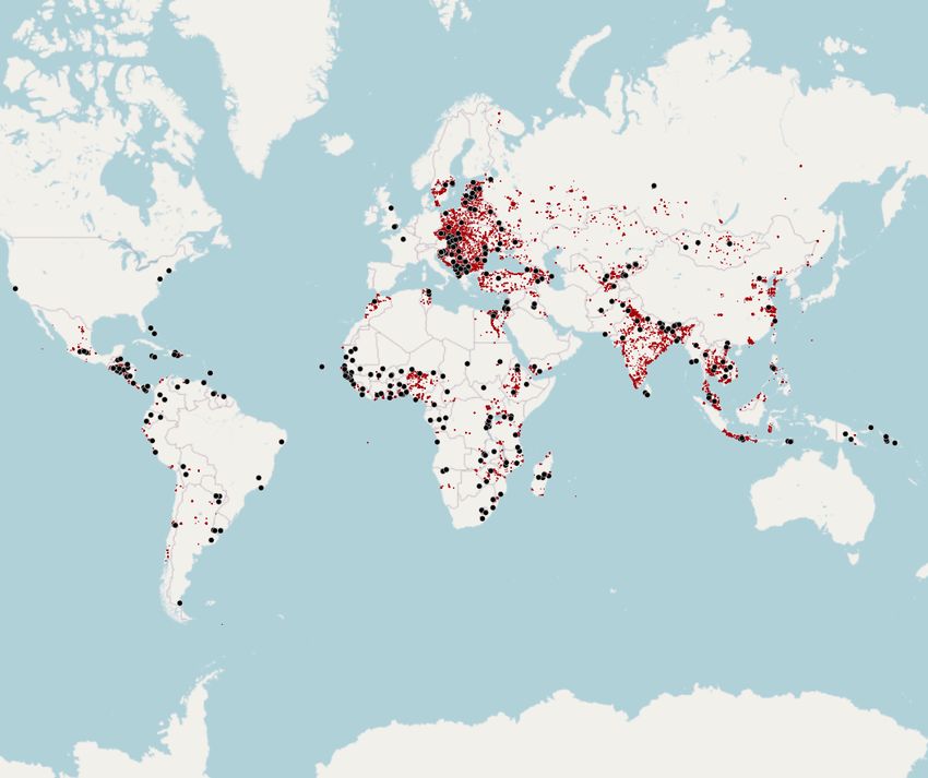
6Figure 1: Leader’s Birthplaces and Firms in Our Sample
N otes : This map presents the geography of our sample and of the identifying variation.
The small red dots represent firms. The large black dots represent circles of 100 km radii
around national leader’s birthplaces. Table A1 presents the list of countries and survey
waves in our sample.3
manually extend these data by including leaders from 2016 to 2020. We then utilize a plug-in
that automatically parses a leader’s birthplace to Google Maps’ API, and retrieves the latitude
and longitude of the city or town. We manually validate no matches or faulty matches, which
can arise due to cities sharing the same names, special characters in city names, or other
reasons. We exclude any leader with less than a year of tenure.
We merge this data on leaders to the enterprise data by country. In the geocoded sub-
sample we calculate the distance of every firm to each leader in the sample period. In the
total sample we generate a dummy indicating whether a firm is within a leader’s region. In
the general sample we have a total of 250 leaders coming from 120 countries. The leader
regions are plotted in Figure 1. Since our empirical strategy builds on leader transitions,
3
For our main sample there are around 25,000 African, 40,000 Asian, 20,000 European, 6,000 Middle
American and 10,500 South American firms available.
7our identifying variation comes from a much smaller sample than the 250 leaders. First,
as discussed above, the enterprise surveys have only been carried out 2.5 times within each
country on average. Second, in many countries, especially in less democratic ones, we do
not observe leader transitions within our relatively short sample. Third, in cases when leaders
were born in foreign countries, we do not identify any favored region. Taking into account
these restrictions, our identifying variation comes from 15 countries in the baseline sample
and from 33 countries in the regional sample.
Country characteristics In order to allow for comparisons across countries and for the
interpretation of mean and aggregate values of monetary variables, we transform variables from
local currency units to 2009 USD. For this transformation, we use period average exchange
rates and GDP deflators from the World Bank’s World Development Indicators. To study
whether the effects of favoritism differ with respect to the political and institutional features
of countries, we collect democracy index data from the Polity5 project, as well as data on
corruption perception indicators from Transparency International.
Tradable and non-tradable sector On a general level, the enterprise surveys identify
whether firms belong to the service or manufacturing sectors. At a more granular level, firms
report the ISIC category of their main product or service. We exploit this information to
construct a measure of product tradability, so as to categorize firms into either the tradable
or non-tradable sector. We rely on the micro-founded approach of Chen and Novy (2011)
that ranks the trade costs of 163 industries at the four-digit NACE level.4 We use this
classification and categorize firms ranking 50 or higher as tradable. This exercise leads to
a total of around 26,500 tradable and 75,000 non-tradable firms in our geocoded sample.
We prefer this approach because, as noted by Holmes and Stevens (2014), many product
categories that are considered manufacturing tend to be sold only locally. For this reason we
4
We utilize conversion tables to translate our ISIC rev 3.1 classification to the 4-digit NACE rev.1 classi-
fication of industries.
8reclassify manufacturing sectors with very high trade costs, such as bricks, as belonging to
the non-tradable category.
Sample and summary statistics Table A1 of the appendix presents a detailed description
of our sample. The Table lists countries, years, number of firms, and leaders in our sample, as
well as which countries contribute to the identification of the favoritism effect. In the Figure 1
map, we also visualize data on firms and leaders’ birth regions. Table A2 in the appendix
shows the summary statistics of the variables used in this paper.
2.2 Identification
Empirical strategy Our empirical strategy exploits data on leader transitions and firm
locations for identification. We compare firms located in “favored” areas in the sense of the
current national leader being born in that region, to firms in the same area but in a time
period when the current leader was not in office. Firms located in other non-favored areas
but having similar observable characteristics, such as being in the same industry, serve as our
control group.
As discussed in Section 2.1, our data measures the location of firms either by the exact
geocoordinates of the firm or by the administrative region of its location as reported in the
enterprise surveys. The geocoded specification is preferred over the regional specification, as
the former is more precise and allows us to study spatial effects around the birthplace of the
leader. However, this comes at the cost of losing identifying variation from the longer sample
period. We start by studying firms whose exact geo-locations is available, where we can
identify effects at granular distances. To obtain complementary evidence, we then replicate
this exercise with the larger sample.
9Geocoded data We estimate a difference-in-differences model of the following form:
log(Outcomef,i,r,c,t ) =α + β km · LeaderAreakm
l,c × T ermc,t + (1)
γ · Controlsf,t + τi + µkm
f + λr + ηc,t + f,i,r,c,t
where Outcomef,i,r,c,t is the logarithm of either of the following five main outcome variables:
total sales, number of permanent employees, output per worker, wage per worker, and total
factor productivity (TFP). We estimate TFP by regressing output in terms of sales on input
factor costs and the net book value of land, buildings and machinery.5 We then study the
residual from this regression as an outcome in equation (1). Our unit of observation is the
firm f belonging to industry i located in region r of country c in year t.
The β km is our main coefficient of interest. It is identified by the set of dummy variables
LeaderAreakm
l,c , which set firms to be treated if they are located within a km kilometer radius
to the birth town of leader l in country c. The superscript km ranges from 10 to 100 km
around the leader’s birthplace in 5 km intervals. Firms located in country c but outside a
150 km radius of the leader l’s birthplace serve as our control group. To get at the average
treatment effect, we interact LeaderAreakm
l,c with T erml,c,t which is a dummy indicating
whether leader l is currently in office.
Controlsf is a vector of firm specific control variables including the age of the firm,
and its ownership shares belonging to foreigners or to the public sector. τi , µkm
f , λr and
ηc,t are industry, leader area, region and country-by-time fixed effects, respectively. The error
term is captured by f,i,r,c,t which we two-way cluster at the level of country-sector-year and
leader area following the arguments laid out by Abadie et al. (2017) to cluster based on the
assignment to the treatment. This clustering strategy is also in line with the design used
by De Haas and Poelhekke (2019), who study the effects of mining activity with the same
firm-level data source and similar time and spatial dimensions as our paper.
5
We sum up the costs for various input factors such as labor, raw materials and intermediate goods or
electricity. As we use total sales as output in this regression, it constitutes as a revenue based TFP measure.
10Regional data As discussed above, we also estimate a version of equation (1), where the
treatment is defined based on the birth region of the leader. The equation is as follows:
log(Outcomef,i,r,c,t ) =α + β · LeaderRegionr,c × T ermc,t + (2)
γ · Controlsf,t + τi + λr + ηc,t + f,i,r,c,t
where the treatment status of a firm is defined by LeaderRegionr,c which is a dummy variable
indicating whether any national leader was born in region r or not.
Identifying assumptions Our difference-in-differences model compares firms located within
areas or regions around the leader’s birthplace before and after the leader comes to power
while controlling for firms belonging to the same industries but located further away from
leader’s birthplace. The main identifying assumption in the difference-in-differences setting
is that the treatment and control groups follow parallel trends prior to the treatment. In our
case, this will be violated if, for example, faster developing regions are more likely to nominate
a national leader. We validate this assumption in Section 4.2 by conducting an analysis that
tests for effects in leads and lags of the treatment variable. We do not find evidence that
any of the several outcome variables between treated and control firms are different from zero
in the years leading to the nomination of the leader. This absence of pre-trends suggests
no systematic bias coming from selection as long as the selection effect is captured by the
observables, and assuming that the selection effect is homogenous across regions so that the
average effect on the pre-trends does not mask potentially offsetting trends. This evidence is
consistent with previous work that has used regional level data to study patterns of regional
favoritism and, similar to our test, finds evidence against the existence of pre-trends.
113 Micro evidence
3.1 Results by distance
We start by studying the treatment effects of favoritism using the detailed geolocation of
firms. We are agnostic about the area around the birthplace, which is potentially affected by
favoritism. Therefore, we exploit information on the exact location of firms and, as specified
in equation 1, estimate the treatment effects of favoritism on firm outcomes in a radius going
from 10 km to 100 km around the leader’s birthplace in 5 km intervals. In this preliminary
exercise, which aims to reveal the spatial dimension of our potential treatment effect, we use
the logarithm of total sales as the main firm level outcome.
Figure 2 plots the treatment effects of favoritism by distance to the leader’s birthplace.
The effects are strongest in areas very close, with firms located in a circle of 10 km around the
leader’s birthplace having on average nearly 30% higher sales than similar firms located further
away. These effects decrease by distance and become indistinguishable from zero beyond 70
km from the leader’s birthplace.
The magnitudes of these effects are substantial. Taking into account the number of
firms operating in these areas and the sum of their sales we can calculate the aggregate
effects of favoritism. The favoritism effect leads to an estimated aggregated sales increase
of $25 billion (in 2009 nominal USD). Hodler and Raschky (2014) calculates that leader’s
regions on average have 1% higher GDP in the worldwide sample, but the effects can reach
up to 9% in certain subsamples. We take their approach of mapping the effects on nighttime
light to GDP growth using the correlation coefficient of 0.8 between firm revenues and GDP
growth, as estimated by Cravino and Levchenko (2017). In our case, the corresponding effect
on the favored regions6 is 11% when transformed into GDP growth values.7
6
To be more comparable with Hodler and Raschky (2014), in this back of the envelope calculation we
take the coefficient estimated for regions from Table 2 rather than the coefficient estimated for certain radii
around leader’s birthplaces, as in Figure 2.
7
Following Hodler and Raschky (2014) and other papers in this literature, we study whether the effects
of favoritism are different across countries with different political institutions. In particular, in Table A4 we
interact our treatment effect with the polity score of democracy and a measure of corruption perceptions. To
study potential non-linear effects we also interact with the squared values of these indices. Overall, we do not
12Figure 2: Treatment Effects by Distance to Leader’s Birthplace
Logarithm total sales
N otes : The regression is estimated using equation 1. The red line plots the coefficient β km
estimated for each radius separately. The shaded area represents 95% confidence intervals.
The dependent variable is total sales and is specified in logarithm. All regressions include
fixed effects for leader circles, regions, industries, and country-by-years. Standard errors are
two-way clustered at the level of country-sector-year and leader area.
3.2 Baseline results
For ease of presentation, we define a baseline area of treatment around the leader’s birthplace
and in the rest of the paper present our estimates based on this area, rather than having
to estimate dozens of point effects over distance for each outcome variable. We choose the
baseline treatment area to include firms located within a 50 km radius around the leader’s
birthplace. We do not use smaller radius measurements in the baseline given the trade-off
that we would lose firm observations and therefore statistical power. Also, focusing on a
find evidence in our sample that democracy or corruption either constrain or exacerbate the effects of regional
favoritism. We relay this difference to Hodler and Raschky (2014) on the differences in the sampled countries,
as our selection of mostly low- and middle-income countries is closer to Dickens (2018), who similarly does
not document significant effects in this dimension.
13Table 1: Treatment Effects around Leader’s Birthplace
VARIABLES Log Log Log Log Log Output TFP
Sales Sales Employees Wage per Worker Residual
Treated area 0.2828***0.2139*** 0.1404** 0.0927** 0.0954*** 0.0479***
(0.0892) (0.0749) (0.0588) (0.0436) (0.0173) (0.0080)
Firm age 0.0251*** 0.0192*** 0.0030*** 0.0049*** 0.0067***
(0.0021) (0.0013) (0.0007) (0.0009) (0.0007)
% owned foreign 0.0171*** 0.0102*** 0.0038*** 0.0065*** 0.0050***
(0.0008) (0.0005) (0.0004) (0.0005) (0.0004)
% owned public 0.0174*** 0.0153*** -0.0001 0.0016 0.0048***
(0.0042) (0.0029) (0.0021) (0.0014) (0.0015)
Constant 16.9923*** 16.4067*** 2.8020*** 11.6463*** 13.5864*** -0.1344***
(0.0217) (0.0433) (0.0273) (0.0167) (0.0189) (0.0130)
Observations 70,177 70,177 79,718 66,262 69,524 57,840
R-squared 0.6369 0.6660 0.2582 0.8286 0.7796 0.2995
F 10.06 129.0 148.4 33.30 45.85 785.0
N otes : The regressions are estimated using equation 1. The treatment is set to a 50km
radius around leader’s birthplace. Dependent variables are specified in logarithms. The mean
values of the dependent variables in levels are 6.8 million USD in columns 1-2, 78 employees
in column 3, 7423 USD in column 4, and 104,000 USD in columns 5. USD is measured in
2009 nominal values. All regressions include fixed effects for leader circles, regions,
industries, and country-by-years. Standard errors are two-way clustered at the level of
country-sector-year and leader area.
small radius may allow us to obtain large estimates, but its aggregate implications on the
economy will be relatively inconsequential. On the other hand, we do not use larger circles as,
according to Figure 2, the treatment effect would start to decline. This choice of fixing the
baseline treated area to a 50 km radius is necessarily a selective one. This choice in general
will not matter for the direction of the effects that we identify. While the magnitudes that
we identify may be somewhat affected, our results and interpretation are robust to specifying
other distances.
We present our baseline results in Table 1. The first column regresses log sales on the
treatment variable and fixed effects. In the second column we include key firm characteristics
as control variables. The estimated coefficient is highly significant and implies that firms
located close to the leader’s hometown experience a 21% increase in sales relative to firms
in the other parts of the country. In the third column our dependent variable is the log total
14number of employees. Again we observe highly significant positive effects of 14% on average.
These effects represent a sales increase of $1.5 million and an employment increase of nearly
10 workers for an average firm.
The size of the estimated coefficient for employment is smaller than the coefficient for
sales. Consistent with this, in columns 4 and 5 we find that treated firms pay higher wages
and produce more output per capita. Finally, column 6 of Table 1 shows that treated firms
not only grow in size, but also become more productive, as measured in terms of total factor
productivity.
4 Robustness checks
4.1 Region level results
As discussed in Section 2.2, we prefer to work with data containing information on the geolo-
cation of firms. However, for a quite larger sample of firms, our data only indicates location
at the regional level. This larger sample also uses twice as many leader transitions for identi-
fication than the geolocated sample. Therefore, as a complementary exercise to our baseline
results, we run regressions in which the treatment is defined by region of birth rather than
birthplace. Table 2 shows these estimates using our five main outcome variables of interest.
As expected, the treatment effects become somewhat smaller and less precise. However, in
all cases the evidence for positive and statistically significant effects can be replicated.8
4.2 Effects before and after leader transitions
We conduct placebo estimations to ensure that our results are driven by leader transitions
rather than existing trends in regions. Since we are using a difference-in-differences specifi-
cation, we want to make sure that there are no pre-trends that potentially drive our results.
8
In an additional specification we interact the region treatment with the 50 km area treatment. Table A3
of the appendix shows the results. Not surprisingly we find strongest effects on firms that are located within
a 50 km radius from leader’s birthplace and at the same time belong to the leader’s birth regions.
15Table 2: Treatment Effects in Leader’s Birth Region
VARIABLES Log Log Log Log Log Output TFP
Sales Sales Employees Wage per Worker Residual
Treated region 0.1543***
0.1308** 0.0609** 0.1013*** 0.0662** 0.0190*
(0.0581)
(0.0512) (0.0290) (0.0343) (0.0280) (0.0111)
Firm age 0.0257*** 0.0195*** 0.0032*** 0.0051*** 0.0060***
(0.0010) (0.0006) (0.0004) (0.0006) (0.0004)
% owned foreign 0.0173*** 0.0103*** 0.0041*** 0.0067*** 0.0045***
(0.0006) (0.0004) (0.0003) (0.0004) (0.0002)
% owned public 0.0176*** 0.0157*** 0.0011 0.0011 0.0034***
(0.0015) (0.0011) (0.0009) (0.0009) (0.0008)
Constant 16.8800*** 16.2709*** 2.7792*** 11.5343*** 13.4884*** -0.1447***
(0.0129) (0.0238) (0.0135) (0.0103) (0.0139) (0.0097)
Observations 126,359 126,359 142,710 121,357 125,191 107,439
R-squared 0.6319 0.6643 0.2626 0.8382 0.7800 0.2741
F 7.048 388.6 499.3 62.28 90.31 149.6
N otes : The regressions are estimated using equation 2. The treatment is set equal to the
administrative region where the leader was born. Dependent variables are specified in
logarithms. All regressions include fixed effects for regions, industries and country-by-years.
Standard errors are two-way clustered at the level of country-sector-year and leader region.
For this reason we construct a placebo treatment variable by assuming that the leadership
transition took place up to two years earlier than it actually happened. In a similar spirit we
also create a treatment variable that takes a value of one for the period covering up to two
years after the leadership transition. We then re-estimate equation (1) including these leads
and lags. The results are presented in Table 3. As can be seen, neither leads nor lags have
significant effects on sales or employment.9
Additionally, the fact that the firm growth effect disappears after the leader leaves office
implies no evidence for the “big push” hypothesis. According to this hypothesis, large positive
shocks and investments can help firms to permanently change their growth trajectories (Mur-
phy et al. 1989), as demonstrated in some recent papers, such as Kline and Moretti (2013),
9
It has to be stated that our data are not well equipped to investigate this issue in more detail due to
the limited frequency with which we obtain the firm-level data. For example, our data also make it difficult
to study tenure (the literature has documented increasing effects with longer tenures). Variation in tenure
would be across countries or leaders rather than between different levels of tenure for the same leader, thus
prohibiting causal interpretation.
16Table 3: Treatment Effects Before and After Leader Transitions
VARIABLES Log Log Log Log
Sales Sales Employees Employees
0-2 years before treatment -0.0697 0.0208
(0.2597) (0.2275)
0-2 year after treatment 0.0248 0.0152
(0.1190) (0.0814)
Treated area 0.1953* 0.2156*** 0.1456** 0.1413**
(0.0992) (0.0766) (0.0721) (0.0609)
Firm age 0.0251*** 0.0251*** 0.0192*** 0.0192***
(0.0021) (0.0021) (0.0013) (0.0013)
% owned foreign 0.0171*** 0.0171*** 0.0102*** 0.0102***
(0.0008) (0.0008) (0.0005) (0.0005)
% owned public 0.0174*** 0.0174*** 0.0153*** 0.0153***
(0.0042) (0.0042) (0.0029) (0.0029)
Constant 16.4122*** 16.4060*** 2.8004*** 2.8015***
(0.0493) (0.0436) (0.0322) (0.0277)
Observations 70,177 70,177 79,718 79,718
R-squared 0.6660 0.6660 0.2582 0.2582
F 105.8 103.4 118.6 120.8
N otes : The regressions are estimated based on equation 1 but adding the leads and lags of
the treatment variable. The treatment is set to a 50km radius around leader’s birthplace.
Dependent variables are specified in logarithms. All regressions include fixed effects for
leader circles, regions, industries, and country-by-years. Standard errors are two-way
clustered at the level of country-sector-year and leader region.
who provide evidence that regional development policies in the US have long term effects, and
Lu et al. (2019), who study China’s successful implementation of Special Economic Zones.
4.3 Country-by-country dropping
We are interested in determining whether the average effects we find are driven by strong
favoritism effects emanating from individual countries. To this end, we re-estimate equations
1 and 2, but successively drop countries with identifying leader transitions one at a time.
Decreases in our coefficient of interest indicate that the excluded country experienced a
17Figure 3: Changes to the Average Treatment Effect from Dropping Countries with Identifying
Variation one-by-one
(a) Specification 1, geocoded data (b) Specification 2, regional data
N otes : The x-axis lists the 3-letter ISO 3166 country code of the country that is dropped
from the estimation for the respective estimate. The red line depicts the average effect of
the corresponding unrestricted samples from Tables 1 and 2.
stronger than average effect compared to the remaining countries, and vice versa. The results
are visualized in Figure 3.
The Figure shows that changes to the average effect are generally small. The largest
increase in both samples is driven by Poland being dropped from the regression, indicating that
the favoritism effect for Poland is below the other countries’ average. On the other hand, the
largest decrease in the geocoded sample stems from dropping Mongolia, and in the regional
level sample from dropping Peru. Size-wise the largest differential is below five percentage
points in specification 1, and below three percentage points in specification 2. Thus, we can
comfortably rule out that our findings are driven by individual countries.
185 Mechanisms
5.1 Sectoral results
We specifically investigate how regional favoritism affects the sectors of the economy, in
order to shed light on a central mechanism behind our baseline results. To this end, we
split firms into the tradable and non-tradable sector. As we discuss in Section 6, we expect
redistributive policies implemented by the government to affect these two sectors differently,
which is consistent with recent findings by Besley et al. (2021), showing that governments have
less leverage to affect firms in the tradable versus the non-tradable sector. In particular, our
model predicts that the non-tradable sector is likely to benefit more from redistributive policies.
This prediction is similar and in line with the literature on inflows of funds to developing
countries from commodity booms, remittances, international aid, or borrowing. Such inflows
increase household incomes, thus boosting consumption. The increased demand for tradable
goods can be met by imports, while demand for non-tradable goods can only be satisfied with
domestic production. Such episodes lead to relative increases in the prices of non-tradable
goods (exchange rate appreciation), the reallocation of factors of production to the non-
tradable sector, and deindustrialization. van der Ploeg (2011) provides a review of the resource
curse literature and its implications. In a more recent study, De Haas and Poelhekke (2019)
investigate the implications of natural resource booms and sectoral reallocation patterns while
also using firm data from the Enterprise Surveys.
In Table 4 we include an additional interaction term between the treatment variable and
a dummy variable for firms in the tradable sector. Section 2.1 describes how we construct this
dummy variable. The results in column 1 show that tradable sector firms located around the
leader’s birthplace benefit less from favoritism. Further, the results in column 2 imply that
they do not experience any growth in output per worker. Column 3 yields similar results for
TFP. In favored areas, productivity growth and growth in output per worker are completely
driven by firms in the non-tradable sector. In column 4 we observe that wage growth is similar
in both sectors. This is consistent with the idea that there is high level of mobility between
19Table 4: Treatment Effects by Sector
VARIABLES Log Log Output TFP Log Log
Sales per Worker Residual Wage Employees
Treated area 0.2554*** 0.1455*** 0.1018*** 0.1010*** 0.1239**
(0.0692) (0.0201) (0.0145) (0.0387) (0.0487)
Tradable 0.1194** -0.1777*** -0.0805* -0.0942*** 0.2976***
(0.0473) (0.0614) (0.0451) (0.0167) (0.0371)
Treated#Tradable -0.1386** -0.1504** -0.1281** -0.0160 0.0335
(0.0670) (0.0731) (0.0522) (0.0291) (0.0583)
Firm age 0.0257*** 0.0048*** 0.0062*** 0.0030*** 0.0199***
(0.0021) (0.0009) (0.0007) (0.0007) (0.0014)
% owned foreign 0.0174*** 0.0065*** 0.0051*** 0.0039*** 0.0104***
(0.0008) (0.0006) (0.0004) (0.0004) (0.0005)
% owned public 0.0177*** 0.0020 0.0050*** -0.0000 0.0153***
(0.0042) (0.0015) (0.0017) (0.0020) (0.0028)
Constant 16.3595*** 13.6339*** -0.1127*** 11.6720*** 2.7106***
(0.0395) (0.0212) (0.0126) (0.0162) (0.0328)
Observations 70,177 69,524 57,840 66,262 79,718
R-squared 0.6585 0.7731 0.2615 0.8269 0.2374
F 100.00 470.8 265.6 31.65 112.3
N otes : The regressions are estimated based on equation 1 but including an interaction term
between treatment and sectors. The treatment is set to a 50km radius around leader’s
birthplace. Dependent variables are specified in logarithms. All regressions include fixed
effects for leader circles, regions, and country-by-years. Standard errors are two-way
clustered at the level of country-sector-year and leader region.
sectors. And despite the fact that non-tradable firms experience more growth, wage demands
faced by firms in both sectors are similar, because both sectors compete for similar workers.
In column 5 we document that there are no sectoral differences in employment growth.
5.2 Business environment
Next, we try to identify the policies and tools used by leaders to contribute to firm growth
in their region. The enterprise surveys ask questions regarding the constraints that firms face
while doing business. Firms are asked to evaluate certain obstacles to their business on a
five-point Likert scale. We center and normalize these variables to report the results in terms
20of standard deviations in Table 5. In the first column the dependent variable is the average
of all business constraints. The estimated coefficient is positive and significant, indicating
a worsening business environment. However, this measure does not indicate the specific
source of the constraint. Accordingly in the following three columns we study its individual
components. The results show that there is no change in the institutional environment around
the leader’s birthplace. Meanwhile, the estimated coefficients on infrastructure constraints
and input constraints are positive and significant. This implies that firms operating in the
areas around the leader’s birthplace see deficiencies in terms of infrastructure and inputs to
a lesser extent as significant constraints to their businesses. The input constraint concept
itself combines three components, the results for which are displayed in the last three columns
of Table 5. From these regressions we observe that firms around the leader’s birthplace
complain about the lack of land and educated workforce, while the coefficient on the access
to finance measure is not significantly different from zero. In terms of relative magnitudes,
among the several types of business constraints, firms are most concerned about the quality
of the workforce.
Taken together, these results imply that leaders divert resources to their home region
and generate higher demand for output produced by firms in the area around their birthplace.
However, they do not promote sufficient infrastructure development to keep up with the
increasing needs of firms. This result is intuitive because infrastructure investments require
planning and proper project implementation. Such activities require longer time horizons and
more effort than, for example, simply awarding contracts to favored firms. In this way, our
results indicate that leaders are more likely to choose the latter option or similar mechanisms
to promote development in their home region. Infrastructure investments themselves can
increase the incomes of local firms and workers, but do little to expand the infrastructure
stock. Studies have shown that in the presence of limited absorptive capacity – in terms of
skills, institutions, and management – countries are unable to translate every dollar of public
investment into an additional dollar of capital stock (Presbitero 2016).
21Table 5: Effects on the Business Environment around Leader’s Birthtown
(1) (2) (3) (4) (5) (6) (7)
VARIABLES Average Infrastructure Institutions Input Land Finance Workforce
Treated area 0.1133* 0.1558*** 0.0316 0.0979** 0.0879*** -0.0493 0.1919***
(0.0615) (0.0575) (0.0787) (0.0384) (0.0264) (0.0336) (0.0483)
Firm age -0.0011*** -0.0008*** 0.0003 -0.0018*** -0.0025*** -0.0022*** 0.0008***
(0.0003) (0.0003) (0.0003) (0.0004) (0.0004) (0.0004) (0.0003)
% owned foreign -0.0006*** 0.0007*** -0.0009*** -0.0013*** -0.0008*** -0.0024*** 0.0005***
(0.0002) (0.0002) (0.0002) (0.0002) (0.0002) (0.0002) (0.0002)
% owned public -0.0017** -0.0014** -0.0021*** -0.0012** -0.0026*** -0.0005 0.0007
(0.0007) (0.0006) (0.0007) (0.0005) (0.0005) (0.0007) (0.0007)
Constant -0.0004 -0.0276** -0.0080 0.0210* 0.0312*** 0.0663*** -0.0590***
(0.0154) (0.0138) (0.0191) (0.0119) (0.0102) (0.0118) (0.0140)
Observations 65,598 78,826 68,654 76,060 77,954 79,469 79,861
R-squared 0.3969 0.2924 0.3902 0.2806 0.2236 0.1947 0.2354
F 8.105 7.314 9.702 18.79 22.15 34.17 6.004
N otes : The regressions are estimated using equation 1. The treatment is set to a 50km
radius around leader’s birthplace. Dependent variables are indices that have been centered
at zero and normalized with a variance of one. All regressions include fixed effects for leader
circles, regions, industries, and country-by-years. Standard errors are two-way clustered at
the level of country-sector-year and leader region.
Regarding input constraints, the regressions indicate that leaders do not directly affect
the capital market. The increasing complaints about lack of land are rather intuitive because
this factor has a fixed supply and does not increase proportionately with output. Finally, the
result in the last column indicates that the demand for labor outstrips the supply of skilled
workers. This is also consistent with increasing wage levels around the leader’s birthplace, as
presented, for example, in Table 1. It is also worthwhile to note that, in the context of ethnic
favoritism, Dickens (2018) shows that there is no increase in migration to the leader’s ethnic
region. It would therefore appear that adjustment is impaired by frictions to labor mobility.
Specifically, tensions between ethnicities can be one factor hindering labor mobility within
countries.
225.3 Further mechanisms
In Table 6 we explore additional channels that may help us to better understand how regional
favoritism works. First, we consider whether firms located in proximity to a leader’s birthplace
are more likely to secure government contracts. Governments may choose to selectively
award contracts to favored firms. Our estimations confirm this hypothesis. We observe that
firms in the treated area are 2.4% more likely to secure government contracts. In column
2 we observe that sales of firms in which the government has an ownership stake do not
experience a differential increase. However, as indicated in column 3, there is a differential
increase in employment at these firms. This provides further evidence for another mechanism
through which the leader can redistribute resources to his or her home region using national
resources. More specifically, those firms engage in hiring despite the fact that their sales are
not increasing. This is inconsistent with the behavior of a profit maximizing firm, but since
the government has a stake in those firms, it can induce sub-optimal choices. In column 4
of Table 6 we restrict our sample to tradable sector firms and study whether they experience
an increase of the share of sales from exports. The results provide no such evidence. A
positive and significant coefficient would indicate an improvement in competitiveness among
firms located around the leader’s birthplace because of improved infrastructure and public
goods provision. However, since we did not observe such improvements in Table 5, it is rather
intuitive that the exporting prospects of firms in the leader’s region do not improve. In the
following two columns, we study whether firms have introduced new products or processes.
For new products we observe a positive and significant coefficient, while for new processes a
negative one. Our interpretation is that higher consumer incomes can generate more demand
and increase firms’ incentives to introduce new products. However, this horizontal expansion
does not necessarily imply improvements in efficiency.10 As process innovations are more likely
to be associated with improved efficiency, these results make intuitive sense.
10
For example, in the multi-product firm framework posited by Mayer et al. (2014) an exogenous increase
in demand can lead the firm to expand its product scope without any improvement in productivity.
23Table 6: Evidence on Further Mechanisms
(1) (2) (3) (4) (5) (6) (7)
VARIABLES Gov. contract Log Log Share sales New product New process Any informal
secured? sales employees direct exports last 3 years? last 3 years? payments?
Treated Area 0.0240***0.2129*** 0.1391** 0.7587 0.0244** -0.0750*** -0.0504
(0.0041) (0.0750) (0.0588) (0.5011) (0.0118) (0.0031) (0.0329)
Treated#% owned pub. 0.0062 0.0069*
(0.0051) (0.0035)
Firm age 0.0016*** 0.0251*** 0.0192*** 0.0281 0.0010*** 0.0008*** 0.0001
(0.0002) (0.0021) (0.0013) (0.0231) (0.0002) (0.0002) (0.0001)
% owned public 0.0020*** 0.0165*** 0.0143*** 0.0012 -0.0001 -0.0001 -0.0001
(0.0006) (0.0047) (0.0031) (0.0322) (0.0007) (0.0007) (0.0003)
% owned foreign -0.0001 0.0171*** 0.0102*** 0.2772*** 0.0009*** 0.0006*** -0.0000
(0.0001) (0.0008) (0.0005) (0.0240) (0.0001) (0.0001) (0.0001)
Constant 0.1470*** 16.4071*** 2.8025*** 10.1210*** 0.3527*** 0.3908*** 0.3004***
(0.0033) (0.0433) (0.0273) (0.5343) (0.0047) (0.0028) (0.0085)
Observations 78,635 70,177 79,718 21,294 57,205 55,932 80,810
R-squared 0.1013 0.6660 0.2583 0.2330 0.2113 0.2944 0.2736
F 37.07 119.6 143.5 33.55 37.49 3818 0.707
N otes : The regressions are estimated using equation 1. The treatment is set to a 50km
radius around leader’s birthplace. The mean values of the dependent variables from left to
right are 17.8%, 6.8 million USD, 78 employees, 12.9%, 38.2%. 39.4% and 28.9%. All
regressions include fixed effects for leader circles, regions, industries, and country-by-years.
Standard errors are two-way clustered at the level of country-sector-year and leader region.
In the last column the dependent variable indicates whether firms have reported making
informal payments. The estimated coefficient is negative but it is not significant. A negative
coefficient would imply that leaders reduce informal tax collection and provide better treatment
to firms located in the areas around their birthplaces. These informal payments are one
manifestation of policy distortions that have been discussed in the misallocation literature
(Hsieh and Klenow 2009, Restuccia and Rogerson 2008).
5.4 Distribution of firm size
In addition to the average effects of favoritism identified thus far, we are also interested in
whether favoritism differently affects the distribution of firms. Following Hsieh and Klenow
(2009), in Figure 4 we present the histogram of the distribution of firms in terms of total
sales by plotting the distribution of residuals using equation (1). We compare treated firms to
24Figure 4: Size Distribution of Treated and Untreated Firms
N otes : The histogram plots the distribution of firms with respect to log sales for the
treatment and control group.
firms in the control group, whereby the green bars represent the former, and the transparent
bars represent the latter, in order to ease comparison. If the favoritism effects were to change
the distribution of firms, we would expect to observe substantial divergence in the distribution
mass of the two groups. As this divergence is minimal, our descriptive evidence does not
indicate a differential effect of favoritism across the firm distribution.
To investigate this issue further, we construct a 95% confidence interval of the ratio of
the above mentioned residuals standard deviations by bootstrapping. This allows us to detect
whether there are statistically significant differences in the distributions between the groups.
However, there is no such evidence, as the confident interval ranges from 0.979 to 1.004,
critically including the value 1. These results inform our assumptions in the following section,
in which we model homogeneous firms.
256 Aggregate implications
In this section we introduce a simple theoretical framework to facilitate the interpretation of
our empirical findings. We also use this framework to estimate the size of the distortions
caused by regional favoritism, and to quantify the aggregate welfare losses generated by such
policies.
6.1 Framework
We consider a two-region and two-sector economy with perfectly competitive firms. Regions
denoted i ∈ {h, a} are the home region which receives subsidies τh and the rest of the country
a which pays taxes τa to finance these subsidies. Positive values of τi denote taxes and negative
values subsidies. We use the term taxes to refer to τi but this should not be taken literally
because these taxes capture various wedges discussed by Restuccia and Rogerson (2008),
including informal payments for which we saw some tentative evidence in Table 6. Firms in
both regions produce manufacturing goods (m) and services (s) j ∈ {m, s}. Manufacturing
goods are traded across regions and internationally; they correspond to the tradable sector in
our empirical analysis. On the other hand, services are only produced and consumed locally,
and thus match the definition of the non-tradable sector given above. We will assume that
both regions are symmetric. Our data provide evidence in support of this assumption. We
run regressions on outcomes that can proxy the average level of development (output per
worker and wage) and include an indicator variable for circles which produced national leaders
during the study period. The estimated coefficient for this indicator variable turns out to
be very close to 0 and statistically insignificant, which implies that the leader circles are not
systematically wealthier or poorer compared to other places.11
6.1.1 Production
We consider a simple production function
11
Our estimations include country-year fixed effects and exclude observations for circle-years during which
the leader was in office from that circle.
26Yij = Lαij . (3)
such that output Yij is produced by using labor Lij . Both regions are endowed with a
fixed amount of homogenous labor Li which is allocated across sectors competitively. Labor is
perfectly mobile across sectors but immobile across regions. We do not introduce capital into
the production function because our empirical results do not show any differential frictions
in the capital market stemming from regional favoritism. Our empirical results are consistent
with a high level of labor mobility between sectors (Table 4), and low mobility between regions
(Table 1). Also in Table 5 we observed that firms do not face differential constraints to capital
access. Thus, we do not add capital to keep the model more tractable.
The firm’s optimization problem can thus be written as
(1 − τi )pij Yij − wi Lij , (4)
where pij is the price in region i and sector j and wi the wage in region i. Perfect mobility
between sectors implies that firms in both sectors face the same wage demands. We also set
a uniform price for manufacturing goods (phm = pam = 1).
6.1.2 Consumption
Both regions are populated by representative agents who derive utility by combining services
γ
(Cis ) and manufacturing goods (Cim ) given by Ui = Cim Cis1−γ . Agents maximize their utility
subject to budget constraints
pis Cis + Cim ≤ wi Li (5)
6.1.3 Market clearing
The equilibrium requires clearing in labor and goods markets
Lhs + Lhm = Lh , Las + Lam = La (6)
27Chs = Yhs , Ccs = Ycs (7)
Chm + Cam = Yhm + Yam (8)
Finally, the government balances its books, which requires that the amount of tax col-
lected in the non-home regions should equal to the subsidies provided in the home region
τh (phs Yhs + Yhm ) + τa (pas Yas + Yam ) = 0. (9)
6.2 Model discussion
The model yields several predictions that help us to understand the empirical results observed
in Section 3. The key outcome of the model concerns the relationship between the tax rate
and the relative allocation of labor between sectors. The model implies that the share of labor
allocated to the services sector decreases with the tax rate.
∂Lis
< 0. (10)
∂τi
Given that the home region receives a subsidy and the non-home region pays taxes, this
implies that a relatively larger share of labor in the home region will be allocated to the
services sector. The intuition behind this result is rather simple. Since only the tradable
good can be transferred across regions, the wedges introduced by the government require
transfers from the non-home region. The relative supply of the tradable good in the home
region increases because it receives transfers. As a result, it becomes optimal for firms in the
home region to allocate relatively more resources to production in the services sector to meet
consumer demand. Consequently, both regions will have relatively more resources allocated
to one of the sectors compared to the economy without wedges. A concentration of resources
in any of the sectors implies a lower level of marginal physical output in the presence of
decreasing returns to scale. As a result, the implementation of taxes will generate aggregate
losses in the economy.
28You can also read