Fast Extended GCD Calculation for Large Integers for Verifiable Delay Functions

Fast Extended GCD Calculation for Large
 Integers for Verifiable Delay Functions
 Kavya Sreedhar, Mark Horowitz and Christopher Torng
 Stanford University, Stanford, USA
 skavya@stanford.edu, horowitz@ee.stanford.edu, ctorng@stanford.edu

 Abstract. The verifiable delay function (VDF) is a cryptographic primitive that
 requires a fixed amount of time for evaluation but is still efficiently verifiable. VDFs
 have been considered a promising candidate for the core function for blockchain
 systems given these fast verification but slow evaluation properties. NUDUPL is a
 state-of-the-art algorithm for VDFs and revolves around a core computation involving
 squaring within class groups of binary quadratic forms. While prior work has focused
 on fast software implementations for this squaring, few papers have investigated
 hardware acceleration, and no prior works accelerate the NUDUPL algorithm in
 particular. Since the most time-consuming operation in the NUDUPL algorithm is
 an extended GCD calculation, we present an efficient design and implementation to
 accelerate this computation. We conduct a detailed study of the hardware design
 space and build an ASIC implementation for 1024-bit integers in an open-source
 180nm-130nm hybrid technology (SKY130). Our design runs with a 3ns cycle time
 and takes an average of 3.7us per computation. After normalizing technologies for
 comparison, we achieve a VDF squaring speedup of 10X compared to the only prior
 class-group-based VDF accelerator and 4X compared to the Chia Network’s software
 implementation, the highest speedup possible by accelerating only the GCD. We sped
 up the extended GCD calculation by 14X compared to the hardware implementation
 and 38X compared to the software. We make our entire codebase publicly available
 as part of our tapeout with the Efabless Open MPW2 shuttle sponsored by Google.
 Keywords: Verifiable delay function · Extended GCD · Bézout coefficients · Squar-
 ing binary quadratic forms · Class groups · ASIC

1 Introduction
Computing the greatest common divisor (GCD) is a fundamental operation in num-
ber theory with wide-ranging applications in cryptography. As a result, considerable
work was conducted in the 1980s and 1990s on developing fast GCD algorithms, pri-
marily building from Euclid’s division [Sor95, Jeb93, Jeb95] and Stein’s binary GCD
algorithms [Ste67, Pur83, BK85, YZ86]. With the recent introduction of verifiable delay
functions (VDFs) [BBBF18] in 2018, there is a new need to develop faster implementations
for computing the extended GCD by finding Bézout coefficients ba , bb : ba ∗ a0 + bb ∗ b0 =
gcd(a0 , b0 ) as most of VDF evaluation runtime is spent on GCD computations. To address
this, we use modern algorithmic and VLSI techniques to reduce the delay of each cycle
in the computation loop and reduce the total number of cycles required for the extended
GCD computation in the context of VDFs.
 VDFs have been considered a promising candidate for the core function for blockchain
systems and are critical to the Chia blockchain design, with the Ethereum Foundation and
Protocol Labs also investigating VDFs and anticipating that they will be crucial to their
designs [Wes18]. There has been demonstrated interest in the cryptography community

2 Fast Extended GCD Calculation for Large Integers for Verifiable Delay Functions

to develop fast VDF implementations with the Chia Network’s Competition promoting
the search for efficient software implementations [Net19]. VDFs are further useful for
adding delay in decentralized systems to avoid adversarial data manipulation for a variety
of applications detailed in [BBBF18] due to their fast verification but slow evaluation
properties. In particular, VDFs must be efficiently verifiable but require a fixed amount of
time to be evaluated despite any available parallelism [BBBF18]. The VDF construction is
defined by three algorithms to setup, evaluate, and verify the function, where the evaluation
may output a proof to aid with the verification. VDFs must be unique (such that the
probability verify returns True for an output that is not the result of evaluate is negligible)
and sequential (an adversary cannot differentiate between the output of evaluation less
than a fixed amount of time steps). Prior works show that exponentiation in a group of
unknown order such as an RSA group or a class group satisfies these properties, resulting
 T
in a widely adopted VDF, f (x) = x2 , which requires T sequential squarings [BBF18].
 While VDFs based on RSA groups are simpler with hardware acceleration explored
in a few early works [Öz19, MOS20, San21], these require a trusted setup. In contrast,
VDFs based on class groups of unknown order do not require a trusted setup and are
therefore preferable over RSA groups. However, only one brief prior work explores hardware
acceleration to date [ZST+ 20]. Furthermore, [ZST+ 20] accelerates the squaring algorithm
described in [Lon19] from the first round of Chia Network VDF competition, but during
the second round, the more efficient NUDUPL algorithm [JvdP02] was adopted instead.
As shown in Figure 1, the extended and partial GCD parts take 76% of the total squaring
runtime in the NUDUPL algorithm, so we focus on accelerating the extended GCD
computation for this algorithm. In the context of VDFs, faster runtimes are the
primary focus as the area and power cost of hardware evaluating a sequential
computation will be negligible compared to the significant costs of blockchain
systems based on proof of work. Our focus in building this chip was therefore primarily
runtime, and we intentionally trade off power and area as described in Section 3 for better
performance.
 Specifically, we make the following contributions:
 1. We present an efficient extended GCD hardware design with an extremely short
 cycle time which uses carry-save adders and minimal control overhead, and reduces
 the number of required cycles.
 2. We release an open-source design and code base for the first hardware accelerator
 targeting the extended GCD computation in the NUDUPL algorithm for VDFs based
 on class groups to enable future researchers in VDF hardware acceleration. 1
 3. We evaluate an ASIC implementation of our extended GCD algorithm in an open-
 source 180nm-130nm hybrid technology (SKY130) that achieves a VDF squaring
 speedup of 10X compared to the only prior class-group-based VDF accelerator and
 4X compared to the Chia Network’s software implementation (the highest possible
 speedup with accelerating only the GCD) as well as an extended GCD speedup of
 14X compared to the accelerator and 38X compared to the software
 In this paper, we first introduce squaring binary quadratic forms over a class group, the
NUDUPL algorithm, and related work on GCD algorithms and accelerating large-integer
arithmetic operations in Section 2. We then describe the guiding decision for our extended
GCD implementation and the tradeoffs we make to prioritize fast runtimes for the VDF
application in Section 3. In Section 4 we evaluate our design and compare our work to the
only prior VDF hardware implementation [ZST+ 20] and an efficient C++ implementation
based on the results of the first round of the Chia Network Competition [Net19]. We
conclude in Section 5.
 1 Code base with parameterized models, scripts, and open-source GDS will be released upon publication.

Kavya Sreedhar, Mark Horowitz and Christopher Torng 3

2 Preliminaries
2.1 Squaring Binary Quadratic Forms over a Class Group
As the Chia Network’s reference on binary quadratic forms [Lon19] explains, a binary
quadratic form is in the form:

 f (x, y) = ax2 + bxy + cy 2 (1)

Our application focuses on integral forms where a, b, cpare integers. The discriminant of
a form is defined as ∆(f ) = b2 − 4ac, with a, b, c < |d| for all reduced elements of a
class group. Unlike RSA groups, class groups of binary quadratic forms do not require
a trusted setup because the order of a class group with a negative prime discriminant d
such that |d| = 3 mod 4 is believed to be difficult to compute for large d, making the order
of the class group effectively unknown as needed. Thus, implementing this squaring over
a class is advantageous as it does not need a trusted setup. Additionally, in the context
of this VDF, all binary quadratic forms are primitive forms meaning that gcd(a, b, c) = 1.
We refer the reader to the Chia Network’s reference on binary quadratic forms for more
information [Lon19].
 The squaring operation is defined as:

 f 2 (x, y) = f (x, y) ∗ f (x, y)
 = (ax2 + bxy + cy 2 ) ∗ (ax2 + bxy + cy 2 ) (2)
 02 0 0 02
 = Ax + Bx y + Cy

 By multiplying out the terms in the product, we can determine how x0 , y 0 can be
written in terms of x, y such that the result is expressed as a binary quadratic form in
terms of x0 , y 0 instead. We describe the squaring operation as finding the coefficients
(A, B, C) given (a, b, c).
 In Wesolowki’s proposed protocol for an efficient VDF evaluation and verification,
the evaluation algorithm primarily consists of squaring and reduction operations [Wes18].
Figure 1 shows the results of our software profiling, indicating that the squaring operation
comprises nearly 80% of the total runtime and is the key operation to focus on for hardware
acceleration. The only prior VDF hardware implementation [ZST+ 20] accelerates the less
optimal squaring algorithm described in [Lon19] from the Chia Network VDF competition in
the first round. To our knowledge, our work is the first to target the more efficient NUDUPL
algorithm [JvdP02] which was adopted during the second round of the competition.

2.2 NUDUPL Algorithm
The NUDUPL algorithm [JvdP02] squares a binary quadratic form over a class group,
which specifically involves finding (A, B, C) given (a, b, c) for a binary quadratic form. We
include comments about simplifications that exploit the fact that gcd(a, b, c) = 1 in the
specific context of a VDF, and we describe the relative cost of accelerating the large-integer
arithmetic needed in hardware.
 Thus, the operations to implement the NUDUPL algorithm are computing large-integer
multiplication, division / mod, addition / subtraction, and negation, as well as extended
GCD and partial GCD which consist of those operations as well depending on the algorithm
used. As a brief note, two’s complement negation can be implemented as an inversion and
then an addition by 1, so we consider this operation to be a subset of addition.
 We profile the amount of time for these various operations in Figure 1 for a 2048-bit
discriminant yielding 1024-bit a, b, c inputs for 1048576 squaring iterations using Riad
Wabhy’s Python implementation [Wab20], with minor refactoring of the code into functions

4 Fast Extended GCD Calculation for Large Integers for Verifiable Delay Functions

 util: ext_euclid_lr()

 group_ops: mul() 12% Extended GCD
 2.1M calls (2 Bézout Coefficients) 5%
 Multiplication 1.3B calls
 Group Operation 12% of runtime divmod()
 21% (2.1M calls)
 vdf_and_proof 2.1M calls 21% of runtime Built-in divmod function
 (2.1M calls)
 NUDUPL Main 3% 39% of runtime
 623M calls 12% (9.4B calls)
 100% of runtime group_ops: partial() 2.5B calls
 31% Partial GCD
 group_ops: sqr() 8.4M calls
 79%
 8.4M calls Squaring 31% of runtime
 Group Operation (8.4M calls)
 20%
 79% of runtime 5.0B calls
 (8.4M calls) util: ext_euclid_l()
 45% Extended GCD
 8.4M calls (1 Bézout Coefficient)
 76% of the runtime
 0% Runtime 100% 45% of runtime is spent in GCD
 (8.4M calls)
 compute for squaring

Figure 1: Software Profiling for NUDUPL Algorithm – The most time-consuming operations
of the VDF evaluation and verification steps are shown, with infrequent operations omitted
from the graph for clarity. The squaring operation comprises almost 80% of the total
runtime. Within that operation, GCD operations take 76% of the time, split between
45% for the Extended GCD calculation and 31% for the partial GCD operation. This
profiling was run four times with a 2048-bit discriminant yielding 1024-bit inputs for
1048576 squaring iterations.

for clarity in the profiling graphs. We average the results for this setup between four
different runs.
 For our entire discussion, if not specified, we use randomly generated 2048-bit discrim-
inants d : |d| = 3 mod 4 which p yields 1024-bit a, b, c inputs as as all reduced elements
of a class group have a, b < |d|. Until recently, 1665-bit discriminants seemed to be a
reasonable target for VDF applications [HM00]. Recent work, however, suggests that the
discriminants may need to be 6656 bits [DGS20]. We use 2048-bit discriminants (and thus
1024-bit a, b, c inputs) as a starting point and note that our hardware implementation is
parameterizable and can easily generate the larger bitwidth hardware.
 From our software profiling in Figure 1, we observe that GCD operations take 76% of
the total squaring runtime, split between 45% for part 1 (extended GCD) and 31% for
part 3 (partial GCD). As a result, we focus on accelerating the extended GCD operation
for part 1 and since the code is identical for the partial GCD calculation just with different
inputs and termination condition, our ideas can be used for the partial GCD calculation
in part 3 as well. To provide context for our work, we cover prior GCD algorithms and
implementations in detail in the following section.

2.3 GCD Algorithms
We describe prior work on GCD algorithms to provide a reference for where we started from
before applying our algorithmic and hardware optimizations explained in the following
sections. In the following discussion, we use the notation in Table 2 for various variables
in the GCD computation. In particular, the inputs to the GCD computation are denoted
a0 , b0 , the inputs to the main computation loop are denoted am , bm , and the intermediate
variables representing am , bm during the GCD-preserving transformations in the main
computation loop are referred to as a, b.
 Most GCD algorithms either build from Euclid’s Algorithm or Stein’s binary GCD
Algorithm [Ste67]. Euclid’s subtraction algorithm repeatedly uses the fact that gcd(a, b) =

Kavya Sreedhar, Mark Horowitz and Christopher Torng 5

Input : (a , b , c ) 1
Output : (A , B , C ) 2
 3
Precompute L := | discriminant |^(1/4) 4
 5
# Part 1 6
Find y such that # Extended GCD 7
x * a + y * b = G = gcd (a , b ) # | G | = 1 for VDFs 8
 # G = a [ MSB ] XOR b [ MSB ]; ~1 FO4 9
By = a / G , Dy = b / G # dividing by G becomes 10
 # conditional negation = 11
 # fast inversion (1 FO4 ) and 12
 # adding 1 ( XOR : ~1 FO4 ) 13
 14
# Part 2 15
Bx = ( y * c ) mod By # can be implemented as modular 16
 # multip lication or a large 17
 # integer multipl ication followed 18
 # by division or mod , with the 19
 # dividend twice as long as 20
 # the inputs ; relatively expensive 21
 22
# Part 3 23
Set bx = Bx , by = By , # Partial GCD 24
Set x = 1 , y = 0 , z = 0 # Efficient GCD i mp le m en ta ti o ns 25
Partial Euclidean algorithm on bx , by # can be leveraged for this part 26
 while (| by | > L and bx != 0) : 27
 q = floor ( by / bx ) , t = by mod bx 28
 by = bx , bx = t 29
 t = y - q * x 30
 y = x, x = t 31
 z = z + 1 32
 if z is odd : 33
 by = -by , y = -y 34
 ax = G * x , ay = G * y # ax = +/ - x , ay = +/ - y 35
 36
# Part 4 # many chained expensive large 37
 # integer operations 38
if z == 0: 39
 dx = ( bx * Dy - c ) / By # multipl ication followed by 40
 # subtraction then followed by 41
 # division 42
 A = by * by # squaring can be done in parallel 43
 C = bx * bx # with 2 modules 44
 B = b - ( bx + by ) * ( bx + by ) + A + C 45
 C = C - G * dx # conditional negation since G = 1 46
 47
# Part 5 48
else : 49
 dx = ( bx * Dy - c * x ) / By # mu lt ip l ic at io n s can be done in 50
 # parallel 51
 Q1 = dx * y # next 3 lines are necessarily 52
 dy = Q1 + Dy # sequential 53
 B = G * ( dy + Q1 ) # multiplying by G becomes 54
 # conditional negation like above 55
 dy = dy / x 56
 A = by * by 57
 C = bx * bx 58
 B = B - ( bx + by ) * ( bx + by ) + A + C 59
 A = A - ay * dy 60
 C = C - ax * dx 61
 62
return A , B , C 63

Figure 2: NUDUPL algorithm from [JvdP02] – We comment on the use of this algorithm
for VDFs given that gcd(a, b, c) = 1 and the cost of building hardware for these operations
alongside the code.

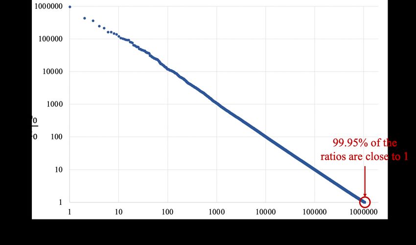
6 Fast Extended GCD Calculation for Large Integers for Verifiable Delay Functions

Table 1: Description and occurrences for cases in the two-bit PM GCD algorithm. Our
techniques build from this algorithm, so we refer to these cases for the rest of this text.
 Case Number Description Rate of Occurrence
 1 a is divisible by 4 10%
 2 a is divisible by 2 (and not by 4) 10%
 3 b is divisible by 4 10%
 4 b is divisible by 2 (and not by 4) 10%
 5 δ ≥ 0 and a + b is divisible by 4 15%
 6 δ ≥ 0 and b − a is divisible by 4 15%
 7 δ < 0 and a + b is divisible by 4 15%
 8 δ < 0 and b − a is divisible by 4 15%

gcd(b, a − b), while Euclid’s division algorithm repeatedly applies gcd(a, b) = gcd(b, a mod
b). The latter is used more often since it converges much faster. Lehmer’s algorithm
was introduced as a more complicated but fast algorithm for large integers that leverages
the fact that most quotients in Euclid’s algorithm are small and the initial parts of the
quotient sequence only depend on the most significant bits of the large input integers.
Later papers have analyzed and sped up Lehmer’s algorithm [Sor95, Jeb93, Jeb95]. Further
work used approximate representations of the numbers based on the most significant bits
to halve the runtime [Jeb93], and was used by the only prior VDF hardware implementa-
tion [ZST+ 20] for the extended GCD calculation (their algorithm did not require a partial
GCD computation but is less efficient overall compared to NUDUPL).
 In contrast, Stein’s binary GCD algorithm [Ste67] uses simpler operations like additions
and shifts instead of divisions which are typically inefficient in hardware. This algorithm
uses the property that gcd(a, b) = gcd(|a − b|, min(a, b)) and removes factors of two from
both or just one number depending on which numbers are even. The Purdy algorithm
[Pur83] utilizes the following GCD-preserving transformations gcd(a/2, b) if a is even and
gcd(a, b/2) if b is even from Stein’s Algorithm, but replaces gcd(|a − b|, min(a, b)) with
gcd( a+b a−b
 2 , 2 ) when a, b are both odd as then a + b and a − b will be even. Brent and Kung
developed the Plus-Minus (PM) algorithm [BK85] based on the Purdy algorithm and keep
track of the binary logarithm representation of the approximate difference in magnitude
between the two numbers, denoted δ in each iteration to determine which GCD-preserving
transformation to utilize. Yun and Zhang introduced the two-bit PM algorithm [YZ86]
which avoids swapping the numbers depending on which number is larger and duplicates
the PM algorithm cases to separately update a and b, eliminates an extra cycle to divide
by four in several cases, and efficiently checks whether a+b a−b
 2 or 2 is odd by using the
second lowest bits of a and b. Thus, the two-bit PM algorithm has eight cases in the
iteration loop as shown in Table 1.
 We used the same VDF software setup for profiling the NUDUPL algorithm as described
earlier and replace the part 1 extended GCD computation with our implementations of
various extended GCD algorithms to generate Table 3. The numbers listed are the average
number of iterations required for the different algorithms for the inputs for this specific
application. From Table 3, we observe that the two-bit PM algorithm takes about twice as
many iterations as Euclid’s algorithm but was intentionally designed for ease of hardware
implementation and consists of simpler operations, namely no mods or divisions, while
Euclid’s algorithm would need a multiplication to implement division.
 In Figure 3, we show the ratios of the inputs for the GCD computation in part 1 of the
NUDUPL algorithm among 4 different 1048576 squarings and observe that 99.95% of the
ratios are close to 1. When inputs are similar in size, Steins-based GCD algorithms are able
to reduce many bits per cycle when the numbers are odd and subtracted from each other
(60% of the iterations in the two-bit PM algorithm as shown in Table 6). While the two-bit

Kavya Sreedhar, Mark Horowitz and Christopher Torng 7

 Table 2: Variable definitions in our design.
 Variables Definition
 a0 , b0 Inputs to extended GCD that returns
 ba , bb such that ba ∗ a0 + bb ∗ b0 = gcd(a0 , b0 )
 am , bm Inputs to the main computation loop, odd by design
 a, b Variables keeping track of the two numbers through
 GCD-preserving transformations in the main computation loop;
 Equal to am , bm at the start of the main computation loop
 α, β Approximations for log2 (a), log2 (b), respectively
 δ Approximation for α − β (which in turn approximates a − b)
 u, m Bézout coefficient intermediate variables such that
 u ∗ A + m ∗ B = a every iteration
 y, n Bézout coefficient intermediate variables such that
 y ∗ A + n ∗ B = b every iteration
 ba , bb Bézout coefficient outputs

 Table 3: Comparison of number of iterations required for various GCD algorithms.
 Algorithm Iterations
 Euclid 597
 Two-bit PM 1195
 Steins 2163
 PM 2857
 Purdy 2951

PM algorithm takes twice as many iterations Euclid’s division algorithm, it has simpler
operations and thus likely faster runtime per iteration and is additionally well-suited for
the inputs for this particular application, so we use this algorithm as a starting point. In
the following section, we describe our work to further reduce the number of iterations and
simplify the operations in each iteration to reduce the critical path length.

2.4 Extended GCD Algorithms
Extended GCD algorithms compute two Bézout coefficients ba , bb such that ba ∗a0 +bb ∗b0 =
gcd(a0 , b0 ) in addition to finding the GCD. GCD algorithms usually consider the case
when the inputs are odd as even factors can be removed or adjusted for earlier before
the main computation loop, so in the following discussion, we denote these odd inputs
as am , bm . Typically, existing GCD algorithms can be extended to calculate the Bézout
coefficients by introducing four intermediate variables u, m, y, n such that the relations in
Equation 3 hold on every iteration. From this equation, we see that at the start, a = am
and b = bm , so the initial values must be u = 1, m = 0 and y = 0, n = 1.

 u ∗ am + m ∗ bm = a
 (3)
 y ∗ am + n ∗ bm = b
 We note that extended GCD algorithms can compute the Bézout coefficients in a
backwards pass once all transformations and control flow to find the GCD are determined
in a forward pass as in [Pur83]. However, this requires twice as many iterations to compute
GCD and Bézout coefficients, so we focus on methods computing only the forward pass.

8 Fast Extended GCD Calculation for Large Integers for Verifiable Delay Functions

Figure 3: Ratio of inputs to GCD computation – Data for the two GCD inputs (a0 , b0 )
for Part 1 of the NUDUPL algorithm when profiled for four different executions with
1048576 squaring iterations each. Since 99.5% of the ratios are close to 1, Steins-based
GCD algorithms will be able to reduce many bits when subtracting the numbers when
they are both odd. Refer to Table 2 for the definitions of a0 , b0 .

 Bojanczyk and Kung present the Extended PM (EPM) algorithm [BB87] that extends
the PM algorithm to calculate the Bézout coefficients with the same control flow. The
authors note that the EPM algorithm appears to be faster than the extended Purdy
algorithm in the average case and is definitely superior in the worst case and that while
asymptotically faster GCD algorithms are known, the PM and EPM algorithms were
the fastest algorithms that could practically be implemented in hardware at the time.
Given that the two-bit PM algorithm is an improved version of the PM algorithm, we
use the authors’ ideas of extending the algorithm in the two-bit PM paper [YZ86] and
the derivation of the EPM algorithm [BB87] from the PM algorithm to build a functional
model for the extended two-bit PM algorithm. Since ultimately a + b will be the GCD, we
note that adding the equations in Equation 3 gives:

 (u + y) ∗ am + (m + n) ∗ bm = a + b = gcd(am , bm ) (4)

 Thus, we can calculate the Bézout coefficients as ba = u + y and bb = m + n at the
end. Since the main computation loop described in these papers was for odd numbers, we
add the two input numbers together if one number is even as suggested in [YZ86] which
results in some small logic accounting for this scenario at the beginning and end.
 We comment on the critical path in the two-bit PM algorithm: if this algorithm is in
cases 5 through 8, as labeled in Table 1, then the Bézout coefficient intermediate values are
added / subtracted together, similar to how a or b is updated with their sum or difference
depending on the case. However, if the Bézout coefficient intermediate values are odd,
the initial odd values to the algorithm are added to this sum or difference to make this
number even and enable the reduction of at least one bit. In cases 5 through 8, at least
two bits are reduced from every number, so in the worst case, three adds are required.
For example, when updating u in cases 5 through 8, the algorithm computes u + y and if
that is odd, computes (u + y) + bm which is even and allows the reduction of one bit to
(u+y)+bm
 2 . If this result is also odd, we add bm again, resulting in (u+y)+b
 2
 m
 + bm (three
additions) which will similarly be even and allow for the reduction of at least one other
bit. Having understood the critical path, we use this extended two-bit PM algorithm as a
starting point for our algorithmic and hardware design decisions.

Kavya Sreedhar, Mark Horowitz and Christopher Torng 9

 Initial Main Loop Final Result
 GCD
a0
 a
b0 ADD b update a a
 4:2 c = a+b c
 CSA
 a0 + b 0 b ADD GCD
 a update b b two's -c
 complement
 am
 c[MSB]
 a0[0]
 Bézout
 bm u
 y
 b0[0] bm update u u
 2bm two's -(u+y)
 3bm 4:2 complement
 2am y CSA u+y
 >> 1 u ADD ba
 bm update y y u+y+n+m
 2bm
 3am 3bm 4:2 two's -(u+y+n+m)
 ADD
 n CSA complement
 m u+y+n+m
 2bm am update n n
 2am n+m
 >> 1
 3am 4:2
 ADD bb
 m CSA two's -(n+m)
 3bm n complement
 ADD am update m m
 2am
 3am Control

 Termination Control am[0] bm[0] c[MSB]

 next a
 loop b update 
 action 
 exit
 a update α α b update β β
 α== 0 & β == 0

Figure 4: Top Level Block Diagram for our Design – The extended GCD computation
begins by initializing variables, iterates in the main loop, and finishes its calculation of the
GCD result and Bézout coefficients. Refer to Figure 5 for update a/b, Figure 6 for update
u/y/n/m, and Figure 7 for update δ. The update α/β modules are explained further in
Section 3.2. Abbreviations: ADD = parallel-prefix adder with carry propagation; CSA =
carry-save adder with no carry propagation; 4:2 CSA = two carry-save adders chained
sequentially to reduce four inputs to two.

3 Accelerating Extended GCD for VDFs
We overview our proposed hardware architecture in Figure 4 with submodules in Fig-
ures 5, 6, 7. Table 2 lists the notation for variables we use throughout this discussion. Our
primary goal was to reduce runtime for the VDF evaluation, and our design decisions focus
on reducing the number of cycles necessary for the GCD computation as well as reducing
the critical path length. This section explores how we modified the extended two-bit PM
algorithm detailed in the previous section to use carry-save adders, approximate binary
logarithm representations, and merging operations to significantly improve performance.
In the discussion below, all numbers refer to working with 1024-bit inputs.

3.1 Addressing Carry-Save Adder Challenges
Carry-save adder (CSA) designs improve the delay of multiple back-to-back additions by
removing carry propagation in all intermediate computations, resulting in O(1) delays
rather than O(ln(number of bits)). This is especially important in wide-word arithmetic,
and is easily accomplished by representing the partial result in a redundant binary form:
two bits are used to represent one bit of the original number. In this form, a number x
is represented by carry and sum, where x = carry + sum. Since the main computation
part of Steins-based GCD algorithms consist of repeated additions between a, b as well as

10 Fast Extended GCD Calculation for Large Integers for Verifiable Delay Functions

 a
 a
 a
 4
 b >> 2 a
 2
 >> 1
 a+b (a+b)
 4:2
 >> 2 4
 CSA

 b-a (b-a)
 4:2 4
 CSA >> 2

 from previous cycle a [1:0]
 from previous cycle b [1:0] Control
 from previous cycle (a+b) [1] Unit
 [MSB]
 
Figure 5: Main Computation Loop Update Block for a and b – Update submodule in the
main loop for a and b. Refer to Figures 8 and 9 for shifting by one and two in redundant
binary representation when using carry-save adders. Abbreviations: CSA = carry-save
adder with no carry propagation; 4:2 CSA = two carry-save adders chained sequentially to
reduce four inputs to two.

u, m, y, n, we can benefit from fast carry-save additions for the majority of the iterations
until a relatively time-consuming final carry-propagate add at the end, reducing the number
of carry-propagate additions needed from O(n) where n is the number of iterations, to
O(1). While prior work has presented GCD algorithms and suggested that carry-save
arithmetic should be utilized for additions in the algorithm [Pur83, YZ86], we found that
actually using CSAs in practice surfaces challenges not addressed in prior works:

 1. With carry-save adders, the critical path of the two-bit PM algorithm discussed in
 Section 2.4 requires four chained carry-save adds and consists of adding bm to u or y
 (and similarly subtract am from m or n) twice so that odd results can be made even
 to enable reducing bits every cycle.

 2. When carry and sum are both odd and a number is shifted in redundant binary
 form, there is a need to efficiently add +1 to get the correct result.

 3. A carry-propagate add is required to add inputs a0 and b0 if either are even, to
 compute two odd inputs am , bm for the initial values of a, b in the main loop.

 4. Another carry-propagate add is required at the end to add carry and sum in
 redundant binary form for the final result of the extended GCD module.

 5. Sign needs to be accurately preserved in redundant binary form since a, b as well as
 u, y, m, n can be negative.

 The carry-propagate add in (3) happens before the main computation loop while the
adds in (4) happen after it has finished. Thus, we run the start and ending modules at 12
the clock frequency of the main clock so that the necessary carry-propagate adds outside
of the main computation loop are no longer contributing to the critical path and our clock
period reflects the benefits of using the faster carry-save additions we use most of the time.
 The carry-propagate add in (2) is required as if the carry and sum representing a
number are odd and then shifted to the right, the inherent truncation associated with the
shift results in an answer that is off by 1 compared to if we shifted (and truncated) and
the original number. Consider the following example:

Kavya Sreedhar, Mark Horowitz and Christopher Torng 11

 from previous cycle a [1:0]
 from previous cycle b [1:0]
 from previous cycle u [1:0] Control Unit
 from previous cycle (u+bm) [1:0]
 u u
 >> 2 4
 y u
 >> 1 2
 bm (u+bm)
 4
 2bm >> 2
 CSA (u+bm)
 3bm >> 1 2

 (u+2bm)
 CSA >> 2 4

 (u+3bm)
 CSA >> 2 4

 update logic when
 a and b are both odd

 u u+y (u+y)
 4:2 4
 CSA >> 2
 y
 (u+y+bm)
 u+y+bm 4
 CSA >> 2
 bm [1]
 (u+y+2bm)
 4
 CSA >> 2
 2bm
 (u+y+3bm)
 4
 CSA >> 2
 3bm

 from previous cycle (u+y) [1:0] Control Unit

Figure 6: Main Loop Update Block for u, y, n, m – Update module for u, y, n, m. The
control signals tapped from a and b are connected at the top level to this module (Figure 4)
from the values for a, b determined by update_a and update_b from Figure 5. Refer to
Figures 8 and 9 for shifting by one and two in redundant binary representation when using
carry-save adders. Abbreviations: CSA = carry-save adder with no carry propagation;
4:2 CSA = two carry-save adders chained sequentially to reduce four inputs to two.

 from previous cycle
 2 ADD 
 from previous cycle -2
 [MSB]

 1
 b [1:0]
 a [1:0]

 -1

 Control Unit

Figure 7: Main Loop Update Block for δ – Update submodule in the main loop for δ. The
control signals that are the lowest bits of a and b are connected at the top level to this
module (Figure 4) from the values for a, b determined by update_a and update_b from
Figure 5. Abbreviations: ADD = parallel-prefix adder with carry propagation.

12 Fast Extended GCD Calculation for Large Integers for Verifiable Delay Functions

 1b
 y w&y
 tmp sum
 1b
sum output
 so sum
 sr w|y sr
 concat
 1b 1b
 w tmp_carry
 output
carry carry
 x | w^y
 co
 cr 1b cr
 x so
 1b
 co 1b

Figure 8: Shifting by 1 in redundant binary form – The design correctly preserves the sign
bit for arithmetic right shift in redundant binary form for use with carry save adders. In
addition, a half adder produces the final LSB to correct for an off-by-1 result when both
the input sum and carry are odd.

 Table 4: Shifting in redundant binary form for a number divisible by 4.

 carry 00 01 10 11
 sum 00 11 10 01
 +1 needed No Yes Yes Yes

 Original number ( num ) Divide by 2: >> 1 1
 ----------------------- ----------------------- 2
 Binary Decimal Binary Decimal 3
 carry = 0011 3 carry = 0001 1 4
 sum = 0011 3 sum = 0001 1 5
 ----------------------- ----------------------- 6
 num = 0110 6 num /2 = 0010 2 != 3 7

 In the example, the result for num/2 should be 3, but shifting the carry and sum
outputs 2 instead. This is because the lower-significant bit information is lost when both
are shifted to the right. In such cases, we must correctively add 1 back to the shifted
result. We note that we cannot simply set the lower bit of carry or sum to be 1, since the
least significant bit for both can already be 1 after a shift (as in the above example). To
correct the shifted result, we use the circuit shown in Figure 8 which consists of a half
adder to add the shifted carry and sum, generating another carry and sum redundant
binary form for the number being represented. The lowest bit of the carry output from a
half adder will be zero by design, so we set that bit to 1 whenever we need to add 1 to
generate the correct result. In this way, we reduce the cost of this correction from the
delay for a carry-propagate add on a 1024-bit input to the delay of just a single XOR gate.
 Detecting the need for this +1 correction is cheap: the AND gate delay in the divide
by 2 case (Figure 8) and an OR gate delay in the divide by 4 case (Figure 9). For divide
by 2, an AND gate checks whether the two lowest bits of carry and sum are set. When
dividing by 4, the two lowest bits of carry and sum have to be one of the combinations
listed in Table 4 for carry + sum to be divisible by 4, so we can simply use an OR gate
for the 2nd lowest bits to detect when to apply this +1 correction. If the OR output is 1
but we are not in one of these four cases in Table 4, then we do not use the calculated
result, so there is no need for extra logic to detect the lowest bits.
 For the chained carry-save additions in (1), we reorganize several computations
from [YZ86] so that we can push pre-computed constants into the start module for
our hardware and eliminate one carry-save add on the critical path. In the two-bit PM
algorithm, the worst-case delay is for the Bézout coefficient update in cases 5 through 8
when the results are repeatedly odd, with the two-bit PM algorithm cases as labelled
in Table 1. For example, that worst-case computation is shown for case 5 on the left in

Kavya Sreedhar, Mark Horowitz and Christopher Torng 13

 y w&y
 1b tmp sum
 1b
 sum s1 output
 sr w^y
 x | w^y concat
 sum
 1b
 sr
 1b
 w
 w&y&x output
carry c1 tmp_carry
 carry
 1b
 cr w|y|x
 x 1b cr s1
 1b c1 1b

Figure 9: Shifting by 2 in redundant binary form – Similar to the shift-by-1 case, the
design correctly preserves the sign bit for arithmetic right shift in redundant binary form
and uses a half adder to produce the final LSB to correct for an off-by-1 result when both
the input sum and carry are odd after 1 shift.

Equation 5. When u + y is odd, we add bm , also odd by design, to make the value even so
we can divide by 2 and reduce a bit. If that result, (u+y)+b
 2
 m
 , is also odd, we again have
to add B to that value for the same reason.

 (u+y)+bm
 2 + bm (u + y) + 3 ∗ bm
 = (5)
 2 4

 We rewrite this expression as shown in Equation 5, noting that the rounding due to
truncating the lower bits when shifting is preserved. Computing the update with the
rewritten expression allows us to push the expensive computation of 3 ∗ B to before the
start of the main loop since that is just a constant. Furthermore, we can avoid this
multiplication by computing 3 ∗ bm = 2 ∗ bm + bm as one shift and one carry-propagate
add in our initial module that is running at 12 the frequency of our main clock and already
computing other carry-propagate adds in parallel. We pre-compute 2 ∗ bm as well and apply
such transformations for all similar computations in cases 5 through 8 so that remove one
chained addition from the critical path.
 Finally, we illustrate how to preserve the correct sign for arithmetic right shifts in
redundant binary form. In prior work, δ represents the difference between a and b to
determine which number is larger and should be updated when both numbers are odd.
However, δ is an approximate representation of log2 (a) − log2 (b) and when incorrect, the
smaller number is updated instead. Because a, b can become negative, there is a need to
properly shift negative numbers in redundant binary form with carry-save adders. We
start with the truth table from [TPT06] that describes the relation between the two most
significant bits of carry and sum before and after shifting to the right, and we determine
relatively balanced equations for computing shifted numbers in this form in Figure 8. This
circuit can be applied sequentially for dividing by four (and similarly for higher powers
of two), but this increases the delay. Instead, we further specialize the logic as shown in
Figure 9 for dividing by four so that the delay is comparable to the divide by two case,
and similar simplifications can be applied for higher powers of two.
 In the main computation loop, all variables except for δ, α, β (with α, β explained
further in Section 3.2) are in redundant binary form. These three variables are small
(ten bits), so the normal adds to update them every cycle do not limit the cycle time.
Additionally, we choose not to keep these control and termination variables in redundant
binary form to eliminate the carry-propagate add that would be necessary to check the
sign of δ for our multiplexer control logic (as well as whether α and β are zero every cycle).

14 Fast Extended GCD Calculation for Large Integers for Verifiable Delay Functions

3.2 Terminating Based on Approximate Binary Logarithms
The termination condition in the two-bit PM algorithm checks whether a or b is equal to
zero to decide to exit the main computation loop. This operation requires many chained
AND gates to check whether all 2048 bits are zero on each cycle. To reduce the number of
bits in this check and the delay in the AND-gate chain, we repurposed α, β from Brent
and Kung’s GCD algorithm in a novel way to determine our termination condition.
 The variables α and β approximate the binary logarithms of a and b and are tracked
through the iterations [BK85] and updated every cycle with the number of bits a and b
will be reduced by at minimum. Thus, when a is divided by 4 or updated with a+b b−a
 4 or 4 ,
the algorithm subtracts 2 from α to approximate the update to a and subtracts 1 from
α when a is divided by 2. Similar updates are performed for β and b. Previously, Brent
and Kung use α and β to compute δ = α − β to approximately keep track of whether a or
b is greater and ultimately store δ directly without storing α and β to avoid performing
this subtraction every iteration. As a result, δ will either increase or decrease by 1 or 2 to
approximate the difference between a and b as shown in Figure 7, depending on which
number was reduced in the last iteration.
 We instead continue storing α and β and use these values in a novel way as an
approximation for a and b in our termination condition as shown in Figure 4. When α or
β is equal to zero, we run our main computation loop one more time (to ensure either a or
b is zero) and initiate final result computation. Since α and β are, by definition, the binary
logarithm of a and b, our algorithm need only check whether log2 (1024) ∗ 2 = 10 ∗ 2 = 20
bits are zero instead of 2048 bits. We still directly store and update δ in addition to α and
β even though δ = α − β to avoid the 10-bit subtraction every iteration.
 However, since α and β are only approximate binary logarithm representations of a
and b, we found that they significantly diverged from the actual values of log2 (a) and
log2 (b). In particular, when a or b is updated with their difference, more than one bit of
the number can be reduced. This is not reflected in [BK85]’s approximate update for α
and β as just 1 is conservatively subtracted from these logarithmic approximations. As
a result, naively changing our termination condition to check α, β instead of a, b added
154 extra cycles for the GCD computation. To mitigate this impact, we experimented
with correcting α and β only occasionally by setting them to be equal to the true values
of log2 (a) and log2 (b) for the a and b at a given point as shown in Table 5. This update
requires a carry-propagate add to convert a and b from redundant binary form, and we
take two cycles for this computation to ensure it is not our critical path. Thus, the increase
to the number of cycles required to support this termination with α, β is due to cycle
increase between cycles added due to using α, β for our termination condition and due to
the extra cycles needed for the correction update. If we apply this correction every cycle
(the first row in Table 5), we get the same results as when the termination condition was
based on a, b since α, β accurately represent a, b every cycle in this case.
 Based on Table 5, we choose to apply this correction once every 64 cycles as that
strikes a balance between minimizing the extra cycles due to using α, β for the termination
condition and minimizing the extra cycles needed for the occasional α, β update that runs
at half the rate compared to rest of the system. With a total average of 1213 cycles, this
change adds a 3.5% overhead to the total number of iterations. We find lower update
frequencies preferable as that requires checking fewer bits every cycle to determine whether
or not we need to make an update. To correct every 64 cycles, we need an AND gate
chain to check whether log2 (64) = 6 bits are zero, which will have less delay than the
10 ∗ 2 = 20 bits that need to be checked to terminate when α or β are zero, so the check
for this correction frequency will not be our critical path.
 Our technique adds minimal overhead while enabling us to perform a fast 20-bit check
for our termination condition instead of the 2048-bit check from prior works, reducing
eleven levels of logic to five.

Kavya Sreedhar, Mark Horowitz and Christopher Torng 15

Table 5: Impact of using α, β for the termination condition – Depending on how often
α, β are updated to be the true binary logarithm of a, b, there is a varying impact on the
number of updates and extra cycles added for the computation. Updating these values
every 64 cycles produces the lowest cycle overhead at 3.5% of total cycles required.
 Update Interval Number of Updates Cycles Added
 1 1194 1194
 16 75 81
 32 38 52
 64 19 43
 128 10 96
 256 5 92
 512 3 346
 Never 0 154

3.3 Reducing Control Overhead
Having sped up the datapath, we must also ensure that the control path does not subse-
quently limit our performance. To accomplish this, we both precompute control signals in
the previous cycle, and duplicate computation to allow the control signals to arrive as late
as possible (late selects) which approximately halve the number of cases to choose from
when we update our variables every cycle.
 The baseline two-bit PM algorithm by design updates either a, u, m or b, y, n every
cycle, and the logic for updating (a, b), (u, y), and (m, n) can be done with the same
hardware with an add or subtract flag (carry in). Thus, one could multiplex the inputs
onto one computation block. In our design, these modules are intentionally duplicated,
as shown in Figure 4, to allow the control signal to arrive late in the cycle. We similarly
apply this parallel computation and late select strategy wherever possible within all the
update modules as well. This performance optimization results in a 40% increase in area.
Since performance is the primary focus in the VDF application domain, we trade off this
area for the faster control path and performance improvement.
 To further remove control delay, we precompute most control signals in the prior cycle.
This is needed since these control signals determine the result for 1028-bit numbers (we
have several extra for intermediate results in the main loop computation to account for
carry bits from repeated addition), so these gates have very high fanout. As a result, when
we ran synthesis, we saw 5 buffers of size 2 to 12 adding 1.53ns of delay to the critical
path. In addition to this buffer delay, for our variables in redundant binary form (all but
δ, α, β) checking whether numbers are even or divisible by 4 is not a direct wiring and
requires some logic (an AND, OR or XOR gate delay) depending on the check.
 We have two types of control signals for our multiplexer logic when determining which
update to use for a, b (Figure 5), control variables such as δ in Figure 7, and the Bézout
coefficient intermediate variables (Figure 6):

 1. Checking bits in an input to a module

 2. Checking bits for an intermediate result (that may be an output) of the module

 Now during a cycle, instead of generating control signals for our mux after we calculate
the various output possibilities that are being muxed (such as whether u+y, computed that
cycle, is even in the update coefficient update pictured in Figure 6 which has a sequential
dependency between this add and the mux control signal), we compute the divisibility
by 2 and 4 of the mux output signal in parallel for our various options and choose the
result for the control logic for the mux in the next cycle. This gives us the a, b, u, y, n, m

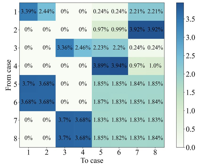
16 Fast Extended GCD Calculation for Large Integers for Verifiable Delay Functions

Figure 10: Frequency of transitions between cases in the two-bit PM algorithm – We show
the transition frequency as the percent of all the transitions in the matrix. The transitions
shown are from the cases on the y-axis to those on the x-axis. For example, transitions
from case 1 to case 2 are 2.44% of all transitions. Refer to Table 1 for case definitions.

related control signals. To similarly compute the a + b, u + y, and n + m control signals
during the previous cycle so that they can just be passed in for the next cycle, we add the
necessary XOR gate for the bits we need for the control signals (the two lowest bits).

3.4 Reducing Cycle Count
The basic operations for the cases listed in Table 1 have widely varying computational
path delays (e.g., dividing by two and four are fast operations). However, since the overall
cycle time is determined by the worst-case operation, many cases inefficiently dedicate
an entire cycle to simple operations. We investigated merging cases with deterministic
transitions to eliminate these inefficient cycles. For example, cases that always produce
an even output can be merged with a divide by two. Although merging cases results in
increased critical path delay, we investigated which mergings would be optimal with a net
benefit for total runtime (cycles ∗ time per cycle).
 The two-bit PM algorithm has a 8:1 mux for determining how a and b should be
updated in the main computation loop as listed in Section 2.3. We note that with the
extended GCD calculation there are additional cases within each branch, but we refer to
this main 8:1 mux in the following discussion for clarity. We show the frequency of each
case in Table 1 and observe that while there is an even distribution among the cases, a and
b are odd slightly more frequently, with cases 5 through 8 occupying 60% of the total cases.
In Figure 10, we show the frequency of transitions between the cases. We note that this
transition matrix is different with and without the optimization in Section 3.2, and in this
section we assume the version with the α, β termination. The matrix is expectedly sparse,
since some transitions can never occur. For example, the algorithm updates a in cases 5
and 6 when a and b are both odd, so it is impossible for the algorithm to transition to
cases 3 or 4 which remove factors of two from b since b will remain odd. We summarize our
optimization experiments based on these transitions in Table 6 and explain them below.

Kavya Sreedhar, Mark Horowitz and Christopher Torng 17

Table 6: Impact of transition-based optimizations on number of cycles, data path length,
and total runtime. X-Y denotes a transition from case X to case Y. We show illustrative
examples of the cases that would be merged in each row instead of listing all the similar
possibilities for clarity. We determine that the optimizations in the bolded rows applied
together provide the best improvement to total runtime, as shown in the last row.
 Transition Optimization Cycles Datapath (ns) GCD Runtime (us)
 Baseline 0 0 3.70
 Merge 5-2 into 5 -236 +0.6 (1 CSA) 3.60
 Merge 7-4 into 7
 Merge 5-2, 5-1 into 5 -374 +1.2 (2 CSAs) 3.62
 Merge 7-4, 7-3 into 7
 Merge 5-2, 5-1, 5-1-1, 5-1-2 -464 +2.4 (4 CSAs) 4.17
 Merge 7-4, 7-3, 7-3-3, 7-3-4
 Add cases: a, b divisible by 8 -65 0 3.52
 Add cases: a, b divisible by 16, 8 -92 0 3.44
 Bolded rows -328 +0.6 (1 CSA) 3.27

 We observe that cases 5 and 6 transition to cases 1 and 2 about one third of the
time to update a (and similarly for cases 7 and 8 to cases 3 and 4) and that these cases
already remove a factor of four from their result. We add a check for whether the result is
additionally divisible by two in cases 5 through 8 and merge the transitions from these
cases to case 2. This optimization has a significant impact, resulting in 236 fewer cycles on
average at the expense of one extra addition along the data path for the Bézout coefficients
calculation and two additional cases (one check for whether the result is additionally
divisible by two, followed by another check for whether the Bézout coefficients are even or
odd) on the control path. We extend this optimization to remove further factors of two in
cases 5 through 8 and see that the incremental benefit in reducing cycles decreases the
more we merge such case transitions. Thus, in terms of total runtime, just one merging
seems to yield the most benefit.
 We also observe that the majority of transitions from case 1 and case 3 (dividing a or b
by four) result in transitions to cases to remove an additional factor of two or four, so we
investigate adding extra cases for when a and b are individually divisible by sixteen and by
eight. We note that while this does increase the worst-case control path as two cases are
added to the 8:1 mux when adding divide by eight (four cases for divide by sixteen and
eight), our critical path is due to the datapath and not control due to our optimization in
Section 3.3. Thus, we use the best version of the odd-to-even case merging optimization
and add the divide by sixteen and eight cases. The net benefit, summarized in the last
row of Table 6, is a 0.44us faster average runtime.

4 ASIC Implementation
We have implemented a preliminary version of our design in an open-source 180nm-130nm
hybrid technology (SKY 130) [GF] with the Efabless Open MPW2 Shuttle [sbG21] as
shown in Figure 11a, with chip parameters in Figure 11b. We use a vertically integrated
methodology spanning cycle-level performance modeling, VLSI-level modeling, and detailed
physical design before taping out our design. We designed our RTL in Kratos 0.0.33 [Zha], a
hardware design language capable of generating SystemVerilog, and we built our testbench
with Fault 3.052 [THS+ 20] to verify our design. In the testbench, 2048-bit discriminants
are randomly chosen to generate 1024-bit inputs for the VDF application as was done for
our software profiling described in Section 2, and we test with randomly generated 1024-bit

18 Fast Extended GCD Calculation for Large Integers for Verifiable Delay Functions

Table 7: Critical Path Breakdown – The critical path is the Bézout coefficient update when
results are repeatedly odd, requiring three back-to-back carry-save additions as shown in
Figure 6. Our critical path delay is 3ns which is 35 inverter fanout-of-4 (FO4) delays as
the inverter FO4 delay is 86ps in SKY130nm technology.
 Operation Standard Cell Delay (ns) FO4 Inv Delay
 DFF clk to Q dfrtp_2 0.54 6.28
 4:2 CSAs for u + y fa_2 0.51 5.93
 fa_2 0.67 7.79
 CSA for (u + y) + 3 ∗ bm fa_2 0.45 5.23
 clkbuf_1 0.11 1.28
 Half adder to correct +1 and2_4 0.13 1.51
 nor2_1 0.09 1.05
 4:1 mux mux2i_1 0.07 0.81
 a211oi_1 0.23 2.67
 8:1 mux nand2_1 0.07 0.81
 nand3_1 0.07 0.81
 Library setup time dfrtp_1 0.07 0.81
 Total N/A 3 35

inputs as well. We use mflowgen 0.3.1 [Tor] for our physical design workflow which relies
on Synopsys DC 2019.03 for synthesis, Cadence Innovus 19.10.000 for floorplan, power,
place, clock tree synthesis, and route, magic [Edw] for DRC, and Mentor Calibre for LVS.
 We identify our critical path in Table 7 as the Bézout coefficient update when the
results are repeatedly odd, which matches our expectations from our earlier analysis in
Section 3. We report a breakdown of this path with delays for each gate in ns. To
help projectour results across different technologies, we also include the delay in units of
inverter fanout-of-4 (FO4) delays [HHWH97] which we have determined to be 86ps in this
technology. We have three carry-save adds along the critical path to compute u + y + 3 ∗ bm .
We note that our optimization from Section 3.1 eliminates an addition on the critical path
by rewriting this update to refactor constants including 3 ∗ bm . In the worst-case scenario,
we must right-shift a negative number and apply an addition +1 with a half adder if the
result was incorrectly truncated when shifting in redundant binary form as explained in
Section 3.1. Finally, the last part of the critical path is the multiplexer logic comprised of
both the inner 4:1 mux and the outer 8:1 mux in Figure 6 as well as the calculation of the
mux control signals for the next cycle as explained in Section 3.3.
 We note that the initial clock-to-Q delay accounts for 20% of our total clock period.
This is a typical value for DFF delays in this library (a high-density library), indicating that
these standard cells are relatively slow in terms of the inverter FO4 delay. Unfortunately,
at the time of our implementation, the high-speed standard cell library for SKY130nm was
still under construction. As a result, our numbers utilize the high-density standard cells,
and our fabricated design takes an average of 3.7us per computation. Based on comparing
the gate delays in our critical path between the high-density and high-speed standard cell
libraries, we estimate that our design would be 40% faster with high-speed cells, resulting
in a critical path of 2.2ns (31 inverter FO4 delays, with one inverter FO4 delay = 71ps for
high-speed library cells in this technology).
 The Efabless Open MPW Shuttle Program [sbG21] allows projects to be 2.92mm2 ∗
3.52mm2 = 10.28mm2 , so we use the full area with a density of 57%, with the chip pictured
in Figure 11a. Our post-synthesis area breakdown is shown in Table 8, with the tradeoffs
between area and runtime described in Section 3.3. Preliminary power estimates indicate
that our design consumes on the order of tens of mW . Recall that in the context of VDFs,

Kavya Sreedhar, Mark Horowitz and Christopher Torng 19

 Technology SKY 130 nm
 Library High density
 Voltage 1.8 V
 Frequency 325.4 MHz
 Synthesized Area 5.66 mm2
 Chip Area 10.28 mm2
 Density 57 %

 (a) Chip Plot of our ASIC (b) Chip Parameters.

 Figure 11: ASIC Implementation

Table 8: Extended GCD Area Breakdown – 68% of the total area is occupied by the
four modules to update the intermediate Bézout coefficient variables due to our decision
to prioritize runtime over area for the VDF application and utilize late select hardware
parallelism (Section 3.3). A traditional JTAG interface is included for chip IO.
 Module Area (mm2 ) % of Area
 Initial computation 0.27 4.8%
 a, b update (2-count) 0.31 5.5%
 Bézout coefficient update (4-count) 3.84 68%
 Control: δ, α, β update 0.57 10%
 Final result calculation 0.36 6.4%
 JTAG 0.22 3.6%
 Miscellaneous 0.10 1.7%
 Total 5.66 100%

area and power overheads for hardware evaluating a sequential computation are far less
important than improving performance (the overheads will be much smaller than the
enormous cost of blockchain systems based on proof of work).
 We compare our design to the only prior class-group-based VDF accelerator by Zhu
et al. [ZST+ 20] in 28nm and the Chia Network’s C++ implementation [Net19] run on
a 2021 Apple M1 CPU in 5nm. Since we used a 180nm/130nm hybrid technology, we
report technology-scaled runtimes for a fair comparison. We use 9.8ps for the inverter
FO4 delay in 28nm [SB17] to calculate the delay ratio between SKY130 and 28nm as
86ps/9.8ps = 8.8, with 86ps as the inverter FO4 delay in SKY130 with high-density
standard cells. Thus, we scale the 6.319us per squaring in 28nm from Zhu et al. to 55us.
 Zhu et al.’s implementation was based on a less efficient squaring algorithm [Lon19]
compared to the NUDUPL algorithm and does not include partial GCD. We achieve
a VDF squaring speedup of 10X and an estimated VDF squaring speedup of
13X with high speed cells by replacing Zhu et al.’s extended GCD module with
ours. We calculate this number by noting that the time spent on non-extended GCD
operations is the time for the total squaring runtime minus the extended GCD runtime,
55us − 53us = 2us. We add this remaining time to the time for our average extended
GCD computation, 3.7us, to get 5.7us and thus a speedup of 55us/5.7us = 10X. Zhu et al.
report that extended GCD calculations took an average of 3000 cycles and a clock period
of 2ns, resulting in 6us on average per extended GCD calculation (53us in 130nm). Thus,
with our extended GCD runtime at 3.7us, We achieve an extended GCD speedup