Examining the soar in the Nasdaq stock market since the COVID-19 outbreak and the influence of retail investors on this rapid price increase.

Examining the soar in the Nasdaq stock market since the COVID-19
outbreak and the influence of retail investors on this rapid price increase.

 By

 Thijs Span†
 Rijksuniversiteit of Groningen
 MSc Finance Thesis
 Supervisor: Dr. J.V. (Jules) Tinang
 2nd reader: Prof. Dr. Wolfgang Bessler
 Date: 03-06-2021

 Abstract
 This paper firstly tests for the presence of a bubble in the tech-heavy Nasdaq stock market since the
 start of the COVID-19 pandemic. Therefore, several econometric tools were proposed: The (i) right-
 tailed augmented Dickey-Fuller test (ADF) by Dickey (1984); (ii) the supremum ADF test (SADF) by
 Philips, Wu, and Yu (2011) and (iii) the generalized SADF by Philips, Shi, and Yu (2013). Using the
 price-dividend ratio (P/D) as time-series data, there is no evidence of an ongoing ‘COVID-19 bubble’
 since the start of the pandemic in March 2020. The proposed tests also show that they are very
 sensitive to different sub-samples. The conclusion is that these econometric tools used for finding
 explosive periods cannot be expected to be a generally valid tool for bubble detection. The tests do
 show good indication for bubble periods, in the perspective of the financial press, but it is yet
 uncertain if an investor would intervene. Therefore, it is important to look at the rationale behind
 explosive periods. The second part of this paper comprehensively investigates the potential factors,
 such as the influence of the upcoming retail investors, that cause the soar in the Nasdaq since the
start of the COVID-19 pandemic. The analysis showed that there is good argumentation, based on the
literature and similarities with previous bubbles, that the tech-heavy Nasdaq stock market is currently
 in the 3rd or 4th phase of a bubble.

Keywords: Stock market bubble, COVID-19, date-stamping, SADF and GSADF tests, retail investors,
explosiveness, Robinhood


 I would like to thank Jules Tinang for his feedback on my earlier drafts and my family for supporting me
through these times.
†
 The author of this paper: Thijs Johannes Julius Span. Currently studying at the University of Groningen, Faculty
of Economics and Business, MSc Finance (EBM866B20.20-2021.2). Contact: T.j.j.span@student.rug.nl

1. Introduction
Technology stocks have seen unpredicted gains in 2020, leading that some may speculate a
bubble that is similar to the dot-com bubble in the late 1990s. The markets have rebounded
sharply after the meltdown in March 2020, when coronavirus was firstly spreading quickly in
the US. Since that period, the Nasdaq composite (.IXIC) has soared about 90%. With the
Nasdaq jumping from its deep valley to its peak in September, in the middle of an economic
crisis, another tech-bubble seems to be forming.
 Figure 1
Graphical evidence of the rapid price increase of the Nasdaq composite (.IXIC) since the start of the COVID-19 pandemic.
Data obtained from Thomson Reuters.

 NASDAQ Composite (.IXIC)
 14500

 13500

 12500

 11500
 Price

 10500

 9500

 8500

 7500

 6500

 Date

The dot-com bubble was very famous for bringing in more liquidity in the form of retail
investors, who took advantage of novel trading platforms to get easily involved with tech-
stocks (Weber, 2009). This time, another group of retail investors has stand up. This group is
aided by popular non-fee trading apps like Robinhood, which led to another boom in retail
investing. According to Wall street Journal (2020), Robinhood saw a record of 1.2 million
accounts open in the first few months of 2020.

The dot-com bubble shows many similarities with the current circumstances, but the biggest
difference is that the 2000s markets were regarded as efficient and the economy was
performing soundly. Today, the market is facing a deep recession due to the COVID-19
pandemic which greatly reduced business activity and led to a spike in unemployment.

This thesis is about testing for the presence of a bubble since the start of the COVID-19
pandemic and analyzes the influence of the upcoming retail investors, who are providing a
generous form of liquidity, on this phenomenon.

 1

Earlier proposed techniques for bubble testing focused on only identifying the presence of a
single bubble. Later on, these were extended such that the starting, duration, and end date
of both single and multiple bubbles could be distinguished and recognized.

In practice, these tests can help the decision-making of (retail) investors and portfolio
managers by rebalancing their portfolios in time of bubble periods1. It also helps to
understand the reasons and ways to overcome the financial crisis and reduce systemic risk
(Lee and Philips, 2016). However, the data of the current literature for the proposed bubble
testing procedures for the Nasdaq do not go beyond 2013. This paper contributes to
improving the knowledge in the field by: (i) The extension of the proposed test to more
recent times, with different sub-samples, and linking these data-stamping procedures to the
perspective of the financial press, (ii) Hypothesis testing for a ‘COVID-19 bubble’ in the tech-
heavy Nasdaq stock market and (iii) comprehensively investigating the influence of the
(potential) factors to the cause of the bubble. Instead of limiting to the statistical evidence,
this paper also looks at the rationale behind explosive periods.

In the next section, the various econometric tools for detecting bubbles from the current
field of knowledge will be reviewed in chronological order. Also, outcomes of similar
research in the previous literature will be discussed. Next, a simple asset pricing model is
proposed that shows the rationale behind time series tests for asset pricing bubbles. This
serves as a theoretical foundation for the Methodology. Subsequently, the Methodology is
explained for the three types of bubble detection test proposed from the literature review.
These are the (i) right-tailed augmented Dickey-Fuller test (ADF) by Dickey (1984); (ii) the
supremum ADF test (SADF) by Philips, Wu, and Yu (2011); and (iii) the generalized SADF
(GSADF) by Philips, Shi, and Yu (2013). The following research question is stated in Section
4.1, with their corresponding hypotheses:

‘’Is there empirical evidence of a ‘COVID-19 bubble’ in the tech-heavy Nasdaq stock market
and what is the influence of the upcoming retail investors on this phenomenon 2?’’

The data section explains which time series data is added and where is it obtained, also the
sub-samples are stated. Next, the results of the three proposed tests are reported. The latter
of the research question will be analyzed in the discussion section. Lastly, the conclusions
are offered.

1
 E.g., following the buy-low sell-high investing strategy: An investor should take a short position in
stocks that are currently in a growing bubble. On the other hand, an investor should take a long
position in stocks after the bubble period.
2
 Refers to the rapid price increase of the Nasdaq composite index (.IXIC), as shown in Figure 1.
 2

2. Literature review
From 1997 till March 2000, during the internet revolution, technology stocks rose more than
five-fold. The introduction of new technology, and the potential economic implications
associated with it, caused overoptimism among many fairgoers. As they soon started to
trade tech related stocks in a purely speculative manner, counting on an everlasting price
increase to buy low and sell high. This caused that the Nasdaq index rose to its all-time peak
of 5,000 in March 2000. On that point, the Dot-Com bubble broke and following that the
Nasdaq index fell by 76.81% to 1,139.90 by Oct, 2002.

In economic studies (financial) bubbles 3are often described as the part of an asset price
movement that cannot be explained on its fundamentals. Although the, previously
discussed, dot-com bubble serves as extremely solid evidence for bubbles, many economist
deny the existence of those bubbles. The dominant paradigm in economics, the Efficient
Market Hypothesis (EFM) (Fama, 1965), states that all information about the fundamentals
of an asset are reflected in the market price through the action of the rational market
participants. Hence, the fundamental value and the market value must be the same.
Otherwise, there would be an arbitrage opportunity (an opportunity to make a riskless
profit) which would be quickly traded away.

LeRoy and Porter (1981) first developed a variance bound test, which is one of the first
options developed for identifying financial bubbles. This variance bound monitored the
present value models, under the assumption of rational bubbles. The model evaluates the
present value of the dividends model, suggesting that the rejection of the present value of
the dividend model is consistent with identifying bubble behavior. Since the variance bound
test is outdated and has some serious problems, this will not be used in this research to
conduct bubble testing. Firstly, in the variance bound test Leroy and Porter (1981) treat
equity prices and dividends as a bivariate process, constructing estimates of variances with
standard errors. Also, it tests as a joint hypothesis – the test simultaneously rejects the
present value model, hence cannot reject the hypothesis of the absence of bubbles. Finally,
the study of Kleidon (1986) shows that the variance bound test fails when dividends and
stock prices are non-stationary.

3
 The definition of a bubble, in terms of this paper, refers to the situation where prices of assets rise
exponentially over a period of time, in excess of their companies’ fundamental value (e.g. their
earnings). These bubbles can include in single stocks, asset classes or a whole stock market. Stock
market bubbles, particularly, can evolve to a more general economic bubble.
 3

To overcome the pitfalls of the variance bound test, West (1987) proposed a variation of the
variance bound test. He calculates the fundamental values of equities as the discounted
present value (DPV) of dividends. For this test he used two null hypotheses. The first null
hypothesis assumes that the stock price is set in accord with a standard efficient market
model. The second null hypothesis assumes that the combination of the efficient markets
model and a speculative bubble component determines the stock prices. West (1987), states
that these two DPV valuations, under the efficient market model, must be the same under
the assumption that fundamentals drive stock prices. If there is an difference in the two DPV
valuations, this could hint to the existence of a bubble. West (1987) carried out the testing
for S&P 500 index and the Dow Jones index in the 20th century. The results from the test are
that the coefficient contingent on the first null hypothesis are statistically different from the
coefficient contingent on the second null hypothesis. Hence, his results hint at the existence
of bubbles.
Unfortunately, Diba and Grossman (1988) criticizes West’s variation of the variance bound
test because it does not allow the possibility of a bubble starting. Because once a bubble is
found, it never crashes. It only get discretely smaller periodically. Therefore, the bubble is
most likely the result of some unobserved variables.

In response to the unobserved fundamentals in the time-series properties of the data, other
numerous time series methods such as cointegration test (Diba and Grossman, 1988) and
unit root test (Campbell and Shiller, 1988) were proposed to detect speculation in asset
prices. Evans (1991) questioned the ability of these models. He used a simulation method
and indicated that the standard unit root and cointegration test fails to reject the null
hypothesis of no bubble in the presence of periodically collapsing bubbles. The problem is
that (previous) explosive periods are ignored when they are succeeded by larger ones.

More recently, Philips, Wu, and Yu (2011, hereafter PWY) and Philips, Shi, and Yu (2013,
hereafter PSY) developed new bubble detection techniques. These strategies are based on
recursive and rolling ADF unit root tests (Dickey, 1984), that enables to detect the starting
date, duration, and date of bubble burst.
PWY (2011) focus on the price movements of stocks as the key indicator for stock market
bubble detection. They used this econometric approach on the Nasdaq index over the full
sample period from 1973 to 2005, and some subperiods. Their bubble model tests the time
series for bubbles by detecting for any statistically significant changes in stock market prices
to explosive autoregressive behavior. The time series of the model is defined as the stock
prices and dividends of the assets. PWY (2011) applied the augmented Dickey-Fuller (ADF) by
(Dickey, 1984) for the presence of a unit root ( 0 ) in the time series sample, also known as a
non-stationarity process, against the right-tailed alternative of an explosive root ( 1 ).

 4

The ADF test produced results of significant explosive behavior in stock prices over the
period, but failed to detect any explosive behavior with the dividends. In other words, the
study of PWY (2011) shows that a ‘exuberance’ (bubble) instance occurred over the period
because there is explosive price behavior without explosive dividend behavior 4.

However, the ADF can only identify if there are explosive periods in the data, it can’t identify
the starting date, duration, and the time of burst of the bubble. This is where the PWY and
PSY developed strategies come in place, which are variations of the ADF. The method used in
PWY (2011) is a supremum ADF test (SADF), which is based on the sequence of recursive
right-tailed unit root ADF tests. The problem with this test is when there are multiple
bubbles, the SADF has not enough power to identify bubbles and cause compatibility. To fix
the problem in the case of multiple bubbles, PSY (2013) proposed the generalized Sup ADF
(GSADF) test. This method, is based on right-tailed retrospective ADF test, with great
flexibility in terms of setting windows.

The PWY (2011) and PSY (2013) studies showed that rolling and recursive tests are more able
to detect bubbles compared with the other time series methods such as cointegration and
unit root tests5. In Monte Carlo study, Breitung and Homm (2012) compared the several time
series methods for the detection of bubbles in stock markets and find that the PWY strategy
performs relatively well in detection of bubbles. They find evidence for a bubble in the
Nasdaq index at the end of the 1990s (Dot-com bubble).

The above mentioned bubble detection strategies are implemented in some recent papers.
For example, Philips and Yu (2011) use the SADF test to date-stamp bubbles in the US
housing market, corporate bond spreads and oil prices, during the GFC. Bettendorf & Chen
(2013) use the GSADF and SADF test and find empirical evidence of explosive behavior in the
Sterling-Dollar exchange rate. Philips et al. (2015) generalized data-stamping procedure

4
 There has been a lot of studies (Smith, Suchanek and Williams, 1998; Oechssler, Schmidt and
Schnedler, 2007), in which the occurrence of econometric bubbles are tested. In these experiments,
research has been conducted on assets with and without dividend payments. In the study of Smith et
al. (1998) bubbles were found of assets with dividend payments on a regular basis. Thus, one
possible factor of the occurrence of bubbles might be the dividend payments. But, bubbles also occur
in markets without dividend payments. The study of Oechssler et al. (2007) shows that the
occurrence of the ‘tremendous’ Dot-com bubble in 2000, was in a market with new economy stocks
who never paid any dividends.
5
 (Normal) unit root tests, as proposed in Dickey and Fuller (1979), with no right-tailed distribution.
Here, the alternative ( 1 ) test for the presence of stationarity in the time series sample. Instead of
the right-tailed alternative with (mildly) explosiveness.
 5

successfully identified 6several bubbles, such as the internet bubble (Dot-Com bubble) of
1997 and the real estate bubble of 2007.

6
 Indicates that bubble periods found using the PWY and PSY methods are in line with the perception
of the financial press.
 6

3. Theoretical foundation
In this section, the foundation of factors driving the asset prices is explained. This is done by
proposing a simple asset pricing model that shows the rationale behind time series test for
asset price bubbles. The discussed SADF and GSADF testing procedures, under the no-
arbitrage condition 7and the assumption of risk neutrality8, are proposed on the basis of the
well-known present-value stock price model of Campbell & Shiller (1987). This equilibrium
price of an asset is equal to the discounted expected outcome at time t + 1

 1
 = E ( + +1 ),
 1 + +1 (1)

where is the real stock price at time t, is the conditional expectation operator and +1
the dividend payment between time t and t + 1. The constant is the (gross) discount rate,
often refer to as the required rate of return, which compensates investors for taking stocks
with a higher beta.

Following Campbell & Shiller (1988) and Cochrane (2002), the log-linear approximation of
Equation (1) can be obtained:

 = +1 + + (1 − ) +1 − +1 (2)

in which, ≡ log( ) , ≡ log( ) , ≡ log( ) , = 1/[1 + exp( 
 ̅̅̅̅̅̅̅)]
 − and

 1
 = − log( ) − (1 − )log ( )
 −1
With ̅̅̅̅̅̅̅
 − being the average (log) price-to-dividend ratio. This price-to-dividend ratio, also
referred to as P/D ratio, can also be calculated by taking the inverse of the dividend yield.
Dividend yield can be an approximation for a real stock return, since the inflation reduces
the effective dividend yield (Gibson, 2008). In D/P, both the numerator and denominator are
nominal variables. Thus, the inflation effect here get canceled out.

The market fundamental is obtained by rewriting the first-order differential equation (2):
 
 = + (3)
Where,
 − 
 = + (1 − ) ∑∞ 
 =0 +1+ , = lim +1 and
 1− → ∞

7
 According to the ‘Efficient market hypothesis’ (EFM) of Fama (1965). The fundamental value and
the market value of assets must be the same, otherwise an arbitrage opportunity would arise.
8
 The situation where investors are indifferent to risk when making their investment decisions.
 7

1
 ̅̅̅̅̅̅̅
 ( +1 ) = = (1 + ( − ))
 
The quantities = + , and in equation (3) are called the ‘fundamental stock-price’
 
and the ‘rational bubble’, respectively. In the absence of bubble conditions, = .

Solving Equation (2) by forward iteration, expectations and log-linear approximation
(Campbell & Shiller, 1988; Cochrane, 2002) yields the following log price-to-dividend ratio
equation (4).
 ∞
 
 − = + ∑ (∆ +1+ − +1+ ) + lim ( + − + ) (4)
 1− → ∞
 =0
Configuring Equation 4 with rewriting the first-order differential equation (2), the right hand
side of Equation (4) can be decomposed into the following two components,

 − = + (5)

Where the fundamental component, , = + ∑∞ 
 =0 (∆ +1+ − +1+ ) stated in
 1− 

terms of expected dividend growth rate and expected returns. The rational bubble
component, , is the focus of the proposed tests described in this paper.

 = lim ( +1 − + ) (6)
 → ∞

This rational9 bubble component is the situation wherein the stock price highly differ from
their fundamental values, without irrational investors’ behavior. This means that in case of a
rational bubble, even that the investors are aware that the stock price highly differ from
their fundamental values, they still hold on in this market because they believe that a lot of
investors are still unaware of this existence.
Under the transversality condition 10 (Kamihigashi, 2006), lim +1 = 0, the condition of
 → ∞
rational bubble component is ruled out. In other words, the actual price is equal to the
fundamental price. In contrast, existence of a strictly positive bubble component, i.e. the
scenario in which the actual price exceeds the (implied) fundamental price, requires that
investors expect to be compensated, for paying the gap between the real and fundamental
price. They expect that this rational bubble component will grow and believe they get

9
 ‘Rational’ in the sense of stock investors, is that they invest to maximize their income and minimize
the cost. In other words, the investors properly process the available information in the markets and
take the optimal decisions based on this information.
10
 Kamihigashi (2006) refers to the transversality condition as: ‘’The optimality condition that often is
used in combination with Euler equations to characterize the optimal paths of dynamic economic
models’’. Kamihigashi (2006) also further discuss this relationship with asset bubbles.
 8

compensated for the risk they take of that the bubble might ‘pop’ in the future. This
behavioral finance is perfectly compatible with the hypothesis of rational expectations
(Tobón, 2014). Therefore, this is called the ‘rational bubble’ (Caspi, 2017).
 
Under bubble conditions, = + , the explosive behavior will be exhibited in that is
inherent to . According to Diba & Grossman (1988) Equation (6) implies a submartingale
property for , since

 1
 ( +1 ) = ̅̅̅̅̅̅̅
 = [1 + exp( − )] (7)
 
When ≠ 0, the logarithmic component of the bubble grows with a rate of =
 ̅̅̅̅̅̅̅
exp( − ), under the condition that is strictly positive. The proposed model reveals
important insights on random features of − . To this extend, the right econometric test
can be proposed designed to rule out the presence of this rational bubble in the stock price.
In this way, the presence of a bubble can be examined. This is the starting point for the SADF
and GSADF tests, where the explosive behavior in the (log) P/D ratio ( − ), can identify
the presence of a bubble. It should be noted that the stochastic properties of − ,
implied by Equation (4), are determined through the fundamental ( ) and rational
component ( ). Sequentially, the fundamental component is determined by the future
expectations of the logarithmic change in dividend (∆ ) and that of the required rate of
return ( ). If these two are at the maximum cointegration of the first order, explosive
evidence of − confirms the existence of a bubble, i.e. ≠ 0 (Philips et al. 2013).

 9

4. Methodology

As discussed in the literature review, to date, PWY (2011) and PSY (2013) studies are best to
determine the starting date, duration and date of bubble burst. The PWY (2011) and PSY
(2013) studies with their respective proposed SADF and GSADF testing strategy is a variation
on the ADF. The basic objective of the standard Dickey-Fuller test, proposed by Dickey and
Fuller (Dickey and Fuller, 1979), is to test for the presence of non-stationarity in time series.
In other words, it tests the null hypothesis that a unit root is present in the time series
sample. Where unit root refers to non-stationarity in the time series process, also known as
a random walk. The alternative of the hypothesis is that there is stationarity11 in the time
series process. The basic objective of the Dickey-Fuller test is to examine the null hypothesis
that φ = 1, where φ is the autoregressive parameter

 = φ −1 + 12 (8)

PWY (2011) proposes in their paper to replace the alternative of the standard Dickey-Fuller
test, stationarity, to the right-tailed13 alternative testing for an explosive root (Dickey, 1984).
Formally, the null and alternative hypothesis are:

 0 : φ = 1 vs. 1 ∶ φ > 1 (9)

Diba and Grossman (1988) have empirically shown that bubbles exist in stock prices and
suggested to use right-tailed unit root test in order to test the presence of bubbles.
This right-tailed Dickey-Fuller test need to be extended for practical purposes, because the
first-order model (only one lag −1 ) is not always rich enough to capture the data features.
Thus, this paper uses the right-tailed ADF with p lags 14(lag order of the autoregressive
process) and intercept using the Ordinary Least Square (OLS) method. The OLS method
minimizes the sum of squares of differences between the observed variable and those
predicted by the linear function of the independent variable (Brooks, 2019).

11
 In case of stationarity, ‘shocks’ to the time series system will gradually die away. In case of non-
stationarity (random walk) these ‘shocks’ persist in the system and will never die away.
12
 The tests in this paper for the presence of bubbles are based on the time-varying autoregressive
model of order one. Where is a white noise with zero mean and variance equal to 2 . The
constant is omitted.
13
 The standard Dickey-Fuller test (1974) alternative is H1: φ < 1 , i.e. based on stationarity. PWY
(2011); Dickey (1984) flips around this autoregressive parameter to H1: φ > 1, i.e. based on (mildly)
explosive process (identifying a bubble). Thus, the critical values are taken from the right tail.
14
 Further on in this paper, the number of lags will be chosen that minimizes the value of an
information criterion as stated by Brooks (2019).
 10

Equation (7) is the generalized form of the following augmented Dickey-Fuller test
regression:
 
 = φ −1 + ∑ − + (10)
 =1

Where is the price of the Nasdaq (.IXIC), is the maximum numbers of lags, 15 is the
random error component.

Firstly, the right-tailed ADF will be used for the rejection of Equation (9), i.e. it test for the
presence of at least one bubble in the time series sample. After this result, the SADF and
GSADF test will be used to identify the starting date, duration and end of the bubble.

The Supremum Augmented Dickey-Fuller test (SADF) is based on the repeated estimation of
Equation (10) on a forward expanding sample sequence. To illustrate this practically, define
the initial sample window size as = 2 − 1. PWY (2011) considers as given that, the
minimal window size 0 , set the subsample starting point at 1 = 0 and the endpoint at
 2 = [0,1]. For the ADF test, the 1 and 2 are fixed to the range of the whole subsample.
However, the SADF test is based on a fixed starting point and an expanding window, where
 1.8
the initial window size is set by ( ∗ (0.01 + ), where X is the amount of observations.
 √ 
Thus, denoting ADF-statistic for a subsample moving from 1 to 2 by 2
 1 . PWY (2011)
define the SADF statistic as the supremum of the ADF sequence for 2 ∈ [ 0 , 1]

 ( 0) = sup { 2
 1=0 } (11)
 2 ∈[ 0 ,1]

The test exhibits that a bubble occurs when the ADF statistic is above the critical value of the
statistic. The critical values of the SADF can be derived from Monte Carlo Simulations, due to
that they are set by Brownian motion of the stock price movements.
In the literature review it became clear that there is a problem with the SADF test in case of
multiple bubbles in the subsample. Here, the SADF test does not have enough power to
identify the bubbles (PSY, 2013). Therefore, the GSADF will be used in case of multiple
bubbles. The generalized SADF (GSADF) proposed by PSY (2013) is similar to the SADF, but it
is allowing for a broader sample sequence by changing both the starting and ending point of
the recursion.

15
 Normally distributed with zero mean and variance 2 .
 11

Because it allows for more subsamples, it increases the power of the statistic significantly. It
is expressed as

 ( 0) = sup { 2
 1 }
 2 ∈[ 0 ,1] (12)
 1∈[0, − ]
 2 0

4.1 Research question & Hypothesis

Since the start of the COVID-19 pandemic, the Nasdaq composite index rose with 90% in
about half a year (Figure 1). In the intro, it became clear that liquidity played a major role in
the creation of the Dot-com bubble in the late 1990s. This seems very similar to what is
happening now, since there is a big upcoming group of retail investors entering the stock
market by upcoming non-fee trading apps (e.g. Robinhood), which is especially bringing up
this huge group of new investors to the tech market.

The first part of this paper is about finding empirical evidence of a ‘Covid-19 bubble’ in the
Nasdaq stock market by using the discussed ADF, SADF and GSADF tests. Here, the
hypothesis from Equation (9) will be used. The research question corresponding to this
hypothesis is:

‘’ Is there empirical evidence of a ‘COVID-19 bubble’ in the tech-heavy Nasdaq stock market
and what is the influence of the upcoming retail investors on this phenomenon?’’

The latter, also the next part of this thesis is to comprehensive investigate the influence of
potential factors, such as the upcoming retail investors, on this rapid price increase in the
Nasdaq composite index since the start of the COVID-19 pandemic. Similarities to previous
bubbles are analyzed in order to create connection and search for the cause of this soar in
the stock market. A second hypothesis is stated to test about retail investors entering the
market due to the facilitating apps/and or sanatory conditions that have led to lockdowns
and accelerate the digitalization of the economy.

4.2 Data

The period of the COVID-19 pandemic has been set since as the count of the first infections
in America, which time-stamp is from mid-March 2020 till now. In this paper, two time series
will be used, the discussed price-dividend ratio (P/D) and the price index. Most key papers
discussed use the P/D ratio as their time series data, for calculating the SADF of PWY (2011);
and GSADF of PSY (2013). The problem here is that, by testing this time series for the Nasdaq
composite Index, only 50% of the Nasdaq composite index pay any dividend, e.g. Tesla
(TSLA). This means that this ratio can be pretty biased towards stocks that pay dividend in

 12

this index. Thus, the assumption that has to be made for this P/D ratio is that the stocks that
pay dividend in the Nasdaq display the whole Nasdaq. Nelson and Arshanapalli (2016) also
showed that the linkage between the real Nasdaq prices and real dividends has been
substantially reduced during the period of 1983-2014. Therefore, another time series is
added: The price series of the Nasdaq composite Index (.IXIC) will also be used. In this way,
the effect of the different time series can be presented and discussed for the sub-samples.
By adding this time series, another problem that occurs is that the Nasdaq prices is a
nominal stock return, which is not adjusted for inflation over the sample period. In contrast
to the dividend yield, which is a real stock return16. Therefore, the real values of the Nasdaq
price index are calculated, as shown in Figure 2. Figure 3 shows the price-dividend ratio of
the Nasdaq.

Both the data of the dividend yield and price index of the .IXIC are provided by Thomson
Reuters Datastream. The P/D ratio is obtained by taking the inverse of the dividend yield and
normalize the series to 100 at the first observation. Since it is important to have high-
frequency data in identifying bubbles (Homm and Breitung, 2012), the data provided is in
monthly data. The dataset consists of 569 monthly observations covering the period of
January 1974 till April 2021.

 Figure 2 Figure 3
Price index of the Nasdaq composite (.IXIC) in the period Price-dividend Ratio of the Nasdaq Composite index (.IXIC) in the period
1-1-1974 and 1-4-2021. 1-1-1974 and 1-4-2021.
 1-1-1974 and 1-4-2021.

 Price index of the NASDAQ composite (.IXIC) in the period 1-
 1-1974 and 1-4-2021.

The results of the three proposed tests, the right-tailed augmented Dickey-Fuller (Dickey,
1984); supremum ADF (PWY, 2011); and the generalized SADF (PSY, 2013), will be shown for

16
 Dividend yield can be an approximation for a real stock return, since the inflation reduces the
effective dividend yield (Gibson, 2013). Also the Dividend yield is calculated by taking the inverse of
the price-to-dividend ratio(P/D). In D/P (or P/D), both the numerator and denominator are nominal
variables. Thus, the inflation effect here get canceled out.
 13

three different sub-samples. The whole sample (Jan 1st 1974- April 1st 2021), the 1st
subsample (April 1st 2001-April 1st 2021) and the 2nd subsample (April 1st 2009- April 1st
2021). The time-span of these subsamples are chosen because of the similarity done by
previous studies described in the literature review. Also, the study of Homm and Breitung
(2012) show that the PSY and PWY perform better for longer sub-samples. The initial
 1.8
window size for each subsample is set by the equation: ( ∗ (0.01 + ), where X is the
 √ 
amount of observations.
The rtadf 17add-in of E-views calculates the relevant test statistics for each of the exuberance
tests (ADF, SADF and GSADF) and simulates the corresponding exact finite sample critical
values via Monte Carlo methods. In which the explosive behavior in the indexes is
investigated via the test statistics with their corresponding 95% critical value, which are
obtained from 1,000 Monte Carlo replications.

To link the upcoming march of retail investors with the rapid price increase of the Nasdaq,
the dataset of the Robinhood popularity metric is used. This dataset consist of historical data
about the numbers of users that hold a particular stock available on the zero-commission
trading platform Robinhood from May 2018 till August 2020. The metric represents the
unique number of accounts that hold at least one share of the asset. The dataset was
collected from the Robinhood API 18. The dataset consist of hourly data of the numbers of
users, to combine this to the Nasdaq composite index the hourly data was converted to daily
data by averaging the hourly numbers of users that hold a particular stock. Since the
popularity metrics do change over weekends, in contrast to the index, these days are
omitted from the dataset.

17
 Caspi (2017) successfully replicated the results of the SADF test of PWY by implementing the
EViews add-in Rtadf. More information on this can be found in the paper of Caspi (2017).
18
 Robinhood API provided on Robintrack.net. As of August 2020, Robinhood has shut down this API.
The reason of this shut down, according to Bloomberg (2021): ‘’They said the reason they’re doing
this is because ‘other people’ are using it in ways they can’t monitor/control and potentially at the
expense of their users.’’
 14

5. Results
When a stock market bubble occurs, the process continues to grow so that it finally reaches
its peak and bursts. After the burst of the bubble, it does not die instantly, but it begins to
adjust itself to its natural level.
Table 1 shows the rejection of the unit-root hypothesis for all the sub-samples. Hence, the
results show empirical evidence of the existence of at least one bubble in the Nasdaq stock
market for the given periods. The results reject the unit root hypothesis at the 1%
significance level for all the sub-samples. It shows the logical explanation that, with reducing
the sub-sample time span, the outcomes become less significant. With the discovery of at
least one bubble in the sub-samples, the following step can be done: Identifying the starting
date, duration, and end date of the bubble using the SADF and GSADF tests.

 Table 1

Test statistics (3 decimals) of the right-tailed ADF for the Nasdaq composite index (^IXIC) over the three specified sub-
samples . The statistics are computed by including a trend and zero lags. The rejection of the test confirms evidence of at
least one bubble in the time series. The critical values are obtained by 1000 Monte Carlo simulations.

 Test-statistics

 Sub-samples: (i) 1974-2021 (ii) 2001-2021 (iii) 2009-2021

 Results 2.952 0.719 -0.204

 Asymptotic critical values (ADF)

 99% -0.380 -0.233 -0.276
 95% -0.964 -0.850 -1.017
 90% -1.224 -1.138 -1.338

The estimated SADF and GSADF test statistics for the two time series data and different sub-
samples are presented in Table 2. The SADF tests statistics who are not significant, will not
be further tested on the GSADF. The insignificant SADF tests figures are not included in the
Appendix. To identify the specific bubble periods, the backward SADF statistic sequence is
compared to the 95% critical sequence obtained from 1000 Monte Carlo simulations. The
test statistics are computed by including a trend and zero lags.

The SADF test statistic does not exceed the 10 percent right tailed critical value of 0.292,
thus there is no (empirical) evidence of explosive periods in the period 2009-2021 for both
the real Nasdaq price series and the price-dividend ratio series.

 15

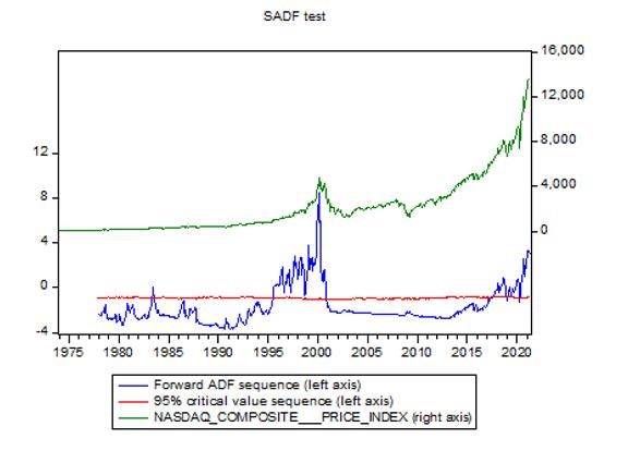
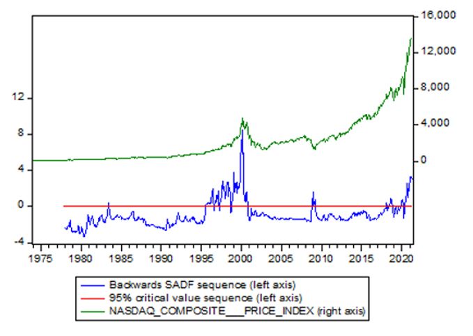
Table 2
Test statistics (3 decimals) for the two exuberance test: The supremum augmented Dickey-Fuller test (SADF) by PWY (2011)
and the generalized supremum augmented Dickey-Fuller test (GSADF) by PSY (2013). The test was performed on the real
Nasdaq price index and price-dividend ratio (P/D) time series data on the three specified subsamples. The test statistics are
computed by including a trend and zero lags. The critical values are obtained by 1000 Monte Carlo simulations.

 Nasdaq price series Price-dividend ratio series
 1974-2021 2001-2021 2009-2021 1974-2021 2001-2021 2009-2021
 SADF 8.441*** 1.035** 0.148 8.989*** -2.094 -1.210
 GSADF 8.662*** 1.622** N/A 9.013*** N/A N/A

SADF tests who are not significant, will not be further tested on the GSADF. This is indicated in the table by N/A. * shows if
significant at the 10% level. ** shows if significant at the 5% level. ***shows if significant at the 1% level.

Looking at the 2001-2021 sub-sample, the SADF test statistic exceeds the 5 percent right
tailed critical value of 1.233, which indicates that the real Nasdaq price series experienced
explosive periods, but is not significant for the price-dividend ratio series. The SADF test
statistic of the 1974-2021 sub-sample exceeds the 1 percent right tailed critical value of
1.897 for both the real Nasdaq price- and the price-dividend ratio series.

It is a pretty obvious observation that picking the sub-sample is very important using these
type of test, as shown in Table 2, Appendix A and confirmed in the study Philips and Shi
(2018). Also, the two time series do show some difference in their results. Since the sample
of 1974-2021 both show evidence of multiple bubbles for the two time series, these will be
further looked into for their date-stamping procedure. This is substantiated by the study of
Homm and Breitung (2012) that GSADF and SADF test perform better for longer-sub samples
(which the result here confirm), especially for identifying stock market bubbles.

Since the figures of the significant SADF test show empirical evidence of multiple bubble
periods, there is justification for using the generalized sup ADF (GSADF) test. As discussed
earlier, the SADF test does not have enough power to identify multiple bubbles (PSY, 2013).
Therefore, the PSY date-stamping procedures will discussed. The figures of the PWY date-
stamping procedure of the SADF test can be found in Appendix A.

Figure 4 shows the PSY date-stamping procedure of the GSADF test for the real Nasdaq price
series. Bubble periods are defined as date points where the sequence of the SADF statistic is
higher than that of the sequence of corresponding 95% critical values. When the SADF
statistic rise above the critical value sequence this is indicated as the start of the bubble
period. After, if the SADF statistic falls below the critical value sequence, this can be
indicated as the end of that particular bubble period.

 16

Figure 4 shows the PSY date-stamping procedure for the real Nasdaq price series, where only
bubble periods longer than 3 months are examined. The 95% critical value sequence here, in
constrast to that of the SADF test, is very close to zero.

 Figure 4
 GSADF test for real Nasdaq price series (.IXIC) between Jan 1st 1974 – April 1st 2021 by including a trend
 and zero lags. This graph includes the Nasdaq series (in green), the SADF statistic sequence (blue) and
 the corresponding 95% critical value sequence obtained from 1,000 monte Carlo simulations (in red).

The results show mainly four date-stamping periods of explosiveness (i) August 1995 – July
1996 (11 months), which can be ascribed to, as discussed in the introduction, (pre)-Dot-com
bubble. (ii) October 1996 – September 2000 (3 year and 11 months), the Dot-com bubble.
(iii) November 2008 – March 2009 (5 months), this period can be ascribed to the short-term
stock market recovery after the Lehman Brothers insolvency in September 2008, also the
well known subprime mortgage crisis (as aftermath of the real estate bubble in 2007). The
first three date-stamping periods are, in general, in line to those reported in other papers
PWY (2011), Homm & Breitung (2012) and with the perception of the financial press. (iv)
April 2020 – still going, this is the possible ‘Covid-19’ bubble, corresponding to Equation 9.

 17

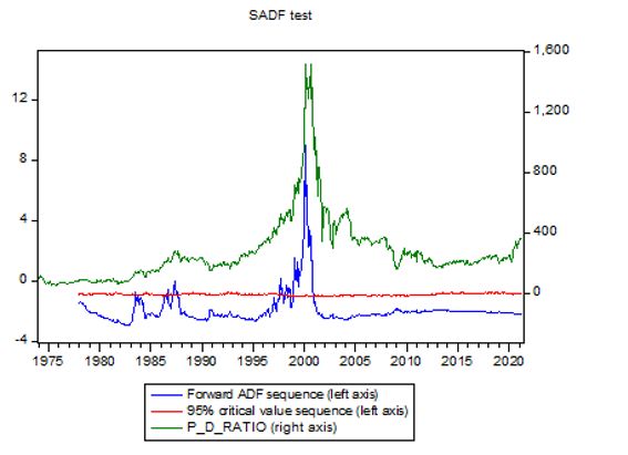
Figure 5
 GSADF test for price-dividend ratio of the Nasdaq between Jan 1st 1974 – April 1st 2021 by including a trend and
 zero lags. This graph includes the P/D series (in green), the SADF statistic sequence (blue) and the corresponding
 95% critical value sequence obtained from 1,000 monte Carlo simulations (in red).

Figure 5 shows the PSY-date stamping procedure for the P/D time series19. The results of the
P/D series show only one big period of explosiveness, (i) January 1999 – September 2000
(1 year and 8 months), the dot-com bubble. These results differ in two ways from the Real
Nasdaq price series. Firstly, the Dot-Com bubble for the price-dividend ratio series is not fully
in line with the perception of the financial press (1997-2001). Second, and most importantly
regarding the first hypothesis of this paper, the price-dividend ratio series show no evidence
of an ongoing ‘COVID-19 bubble’.
The question that now arises: ‘’Which time series do we follow?’’. Following the key papers
(PWY, 2011; PSY, 2013), which use the P/D ratio as time series data, then there is no
evidence of a COVID-19 bubble. However, it must then be assumed that the stocks that pay
any dividend in the Nasdaq, represents the whole Nasdaq in terms of explosiveness. In case
of following the real Nasdaq price series, there is evidence of the COVID-19 bubble. In the
real Nasdaq price series, the date-stamping periods are in line to the perception of the

19
 Here, only bubbles longer than 3 months are discussed. Smaller bubble periods found are: (i) The
stock market crash of 1983 (June 1983- August 1983), (ii) Black Monday in October 1987 (May 1987-
June 1987) and (iii) the subprime mortgage crisis (December 2008).
 18

financial press and similar to that from the key papers (PWY, 2011; Homm and Breitung,
2012). Therefore, the real Nasdaq price series looks like a good alternative. It can be
concluded that results of the SADF/GSADF test are very dependent on the definition of the
sub-sample (Table 2; Appendix A), as earlier confirmed by other papers, and should be
interpreted with caution. For robustness check purposes, the same tests are included for the
S&P 500 in Appendix B.

 19

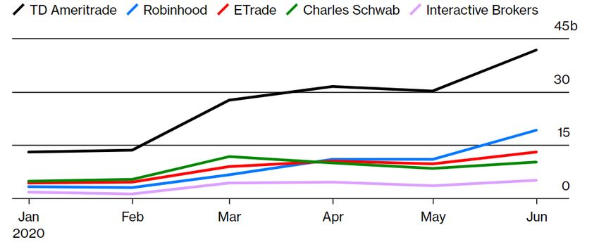
6. Discussion

 Even though the proposed SADF/GSADF test for the P/D ratio time series show no evidence
 of the COVID-19 bubble, this does not take away from the fact that since the start of the
 COVID-19 pandemic Nasdaq is breaking closing records with their rapid price increase
 (Figure 1). The following question that can be stated following this: ‘’ What is the cause of
 this rapid price increase of the Nasdaq stock market index since the start of the COVID-19
 pandemic?’’
 Former president of the Deutsche Bundesbank, A. Weber, said that: ‘’The past has shown
 that an overly generous provision of liquidity in global financial markets in connection with a
 very low level of interest rates promotes the formation of bubbles’’ (Griffiths and Lucas,
 2016, p.119).

 The dot-com era was very famous for bringing in more liquidity in the form of retail
 investors, who took advantage of novel trading platforms to get easily involved with tech-
 stocks. The start of the COVID-19 pandemic created a unique moment for retail investors to
 start trading: Increased market volatility, stay-at-home-orders and, the most important, zero
 commission fees across all trading platforms (e.g. Robinhood).
 According to the Wall street Journal (2020), Robinhood, one of the biggest trading platforms
 in America, saw a record of 3 million new customer accounts open in October 2020.
 Figure 6 shows the rising march of retail equity trading volume in zero-commission trading
 apps since the start of 2020.

 Figure 6
Retail equity trading volume (in shares) for the 5 major trading platforms in the United states. Most of these platforms mainly
trade (tech-)stocks of the Nasdaq stock market. The trading volume is shown since January 2020 till June 2020.

 Source: Bloomberg Intelligence

 20

Robinhood grew from their 3.1 billion trading volume in February 2020 to a 19.3 billion
trading volume in June. This is more than fivefold since the start of the pandemic. Also other
trading platforms noticed the influence of retail investors, the trading volume of TD
Ameritrade rose from 13.6 billion to 41.6 billion and that of Etrade from 4.5 billion to 12.9
billion. As further confirmation of this upcoming march of retail investors, Figure 7 (Appendix
C) shows the market share of overall US equity trading volumes. Here, retail trading has
made a big jump in market share (around 6%) since the start of the COVID-19 pandemic,
such that it accounts for almost as much volume as the mutual funds and hedge funds
combined.

These brokers allows their investors to take leverage in the form of options. Aramonte &
Avalaos (2021) states that the margin debt balances rose with 60% as aftermath of the
pandemic to $750 billion. This is the highest level since that of the Dot-com bubble in 1997,
both in inflation-adjusted terms and as share of GDP. Also, the amount of Initial Public
Offerings (IPOs), which were very popular under retail-investors in the Dot-com bubble due
to their rapid share price increases in the first few days, intensified. The year 2020 saw 480
IPOs exceeding the 406 in 2000 (Source: Stock Analysis).

To link this soar in retail investor with the earlier observed rapid price increase of the
Nasdaq, the popularity metric dataset of the Robinhood API is used. This dataset consist of
hourly historical data about the numbers of users that hold a particular stock available on
the zero-commission trading platform Robinhood. The dataset was converted to daily data,
for combining it with the Nasdaq price index, by averaging the hourly data. The metric
represents the unique number of accounts that hold at least one share of the asset. In order
to draw a conclusion from this, the following assumptions have to be made: (i) The top 1020
largest stocks, which account for one-third of the index performance, display the whole
Nasdaq composite index. (ii) Robinhood investment behavior is a good representation of the
whole retail investors market. The outcome of combing the two datasets is shown in Figure
8.

20
 The top 10 largest stock in the Nasdaq composite Index (.IXIC) by market capitalization according
to Thomson Reuters as of April 2nd 2021 are: 1. Apple (NASDAQ:AAPL), 2. Microsoft (NASDAQ:MSFT),
3. Amazon (NASDAQ: AMZN), 4. Facebook (NASDAQ:FB), 5. Alphabet Class C (NASDAQ:GOOG), 6.
Alphabet Class A (NASDAQ:GOOGL), 7. Tesla (NASDAQ:TSLA), 8. NVIDIA (NASDAQ: NVDA), 9. PayPal
Holdings (NASDAQ:PYPL) and 10. ASML Holdings (NASDAQ:ASML).
 21

Figure 8
Popularity metric of the Robinhood trading-app holders versus the Nasdaq composite index (.IXIC) over the period May-2018 till
August 2020. Data of the Popularity metric is obtained from the Robinhood API and the data for the Nasdaq composite index of
Thomson Reuters Database. Popularity metric represents the unique number of accounts that hold at least one share of the asset, the
stocks series are shown by stacking the areas as chart type.

 Popularity metric versus Nasdaq index
 3500000 12000

 3000000 10000
 2500000
 Popularity metric (holders)

 Price index (NASDAQ)
 8000
 2000000
 6000
 1500000
 4000
 1000000

 500000 2000

 0 0

 Date

 ASML FB TSLA AMZN GOOG GOOGL
 NVDA PYPL MSFT AAPL Index

 This graph shows that the number of unique accounts that at least hold one share of asset
 skyrocketed at the start of the pandemic at March 2020. Apple (AAPL), a very popular stock
 on Robinhood had an average of 171.220 account holders over whole 2019. This number
 increased since March 2020 (200.074 users) to an amount of 683.300 accounts holders.
 Amazon (AMZN) popularity rose with a 106.987 holders in March 2020 to an amount of
 422.076. To clarify, in practice, accounts can have multiple shares of an asset, which will
 make this relation even more convincing. The graph clearly shows that retail investors are
 ‘buying the dip’ of the Nasdaq, at the start of the pandemic. Thus, considering figure 6
 through 8, it can be argued that the form of liquidity retail investors brought in 1997 with
 the Dot-com bubble is similar (or even bigger) to what is happening since the start of the
 COVID-19 pandemic.

 The start of the pandemic led to that the US Federal reserve (Fed) cut their interest rates, to
 boost the economy. Figure 9 shows the 10-year US treasury yield, this is used as a proxy for
 the interest rate in the US economy. This graph indeed show a big decrease in the interest
 rates around the start of the COVID-19 pandemic to a historically low rate of around 0.7%.

 22

Figure 9
The 10-year US Treasury yield over the period September 1998 till April 2021. The 10-year US treasury yield is used as a
proxy for the interest rates in the US economy. When treasury yield increases, interest rates in the economy also increase
and vice versa. The data is obtained from the Thomson Reuters Database.

 The 10-year US Treasury Yield
 8,00%

 7,00%

 6,00%

 5,00%

 4,00%

 3,00%

 2,00%

 1,00%

 0,00%
 1-9-1998
 1-8-1999
 1-7-2000
 1-6-2001
 1-5-2002
 1-4-2003
 1-3-2004
 1-2-2005
 1-1-2006
 1-12-2006
 1-11-2007
 1-10-2008
 1-9-2009
 1-8-2010
 1-7-2011
 1-6-2012
 1-5-2013
 1-4-2014
 1-3-2015
 1-2-2016
 1-1-2017
 1-12-2017
 1-11-2018
 1-10-2019
 1-9-2020
This intervention of central banks is against the classical-Liberal perspective of French
(2009). He thinks when the government pushes the interest rate downward, by changing the
money supply, this encourages investors to invest in ways which they otherwise would not.
Because as interest rates become low, so does the yield on the savings accounts. Such that
this new group of investors, retail investors, fuels a bubble that eventually must burst and
force these malinvestment to be liquidated. The Dot-com bubble of 1997 serves as an
perfect example of interference of the government can encourage unwise investments.
In contrast to this classical-liberal perspective, John Maynard Keynes (1936):
‘’Following the Keynesian perspective, the high drop of rise in asset prices is more based on
human emotion rather than their intrinsic value.’’

Most of the stocks in the Nasdaq composite index are either tech-, internet- or other high-
growth stocks. These differ from value stocks in the way that, value firms profits are typically
expected in the next upcoming years, rather than being spread over the next few decades as
growth stocks are. These growth stocks tend to benefit with a decline in the long-term yield,
as their value of their future cash flow climb.

 23

The proposed tests, following the strategy of the key papers (PWY, 2011; PSY, 2013; Homm
and Breitung, 2012), didn’t show any empirical evidence of an ongoing stock market bubble
in the Nasdaq. But what does the literature say? According to Hyman Minsky (1986), an
economist of post-Keynesian signature, a bubble can be characterized by the following five
phases:

 1. Displacement, a systematic shift that occurs when investors get excited by a
 paradigm, such as new technologies, innovation or even a war. This new
 displacement, in combination with some of the following characteristics, differs stock
 market bubbles from simple bull markets21.
 2. Boom, this is the moment where the asset prices gain momentum, which is
 constituted by low levels of volatility and credit expansion.
 3. Euphoria, the phase where asset prices grow exponentially due to the combination of
 high volume of trades, with upcoming levels of volatility.
 4. Profit-taking, this phase creates slight concerns among investors about the
 irrationality of the market. However, no one knows when the bubble will pop. This
 phase still shows high volume of trades, which are sustained mostly by less
 sophisticated investors.
 5. Panic, this phase is the burst of the bubble, where prices fall rapidly to their
 fundamental values. This is where supply overwhelms demand.

These theoretical characteristics are now referred back to the ‘COVID-19 bubble’. Regarding
the first phase, Bughin et al. (2017) stated that the shift of digitalization of the economy
already took place in 2016. It can be argued that the evolution of non-fee commission apps,
that started in the beginning of 2020, has taken this displacement to an higher level and that
the sanitary conditions that have led to lockdowns fueled this digitalization of the economy
even higher. The second phase, the intervention of the federal government in response to
the start of the pandemic in March 2020. Where interest rate decreased to a historically low
rate at the start of the pandemic (Figure 9). Figure 10 shows the volatility index (.VOLQ) of
the Nasdaq.

21
 A bull market is the condition of financial markets in which the price of assets rises for a long period
of time (months or even years). So, the question that pops up: ‘Why is this not just a (simple) bull
market instead of a bubble?’. The bubble occurrence takes place when the normal bull market gain
stimulus due to a new displacement (e.g. economic policy, innovation, new technology or some
‘Black Swan event’). The difference between the two can be attributed to as market irrationality.
 24

Figure 10
Volatility of the Nasdaq-100 index (.VOLQ) over the period 2019 till April 2021. This index measures changes in the 30 day
implied volatility. This is used as a proxy for the volatility of the Nasdaq. The data obtained is from the Thomson Reuters
Database. In Appendix D the historical volatility of the Nasdaq (.IXIC) is added as confirmation.

 Volatility of the Nasdaq (.VOLQ)
 90
 80
 70
 60
 50
 40
 30
 20
 10
 0

 1-6-2020
 1-1-2019
 1-2-2019
 1-3-2019
 1-4-2019
 1-5-2019
 1-6-2019
 1-7-2019
 1-8-2019
 1-9-2019
 1-10-2019
 1-11-2019
 1-12-2019
 1-1-2020
 1-2-2020
 1-3-2020
 1-4-2020
 1-5-2020

 1-7-2020
 1-8-2020
 1-9-2020
 1-10-2020
 1-11-2020
 1-12-2020
 1-1-2021
 1-2-2021
 1-3-2021
 1-4-2021
This shows very low levels of volatility around the start of the pandemic, thus perfectly
matching with the characteristics described in the Boom phase. Sornette et al. (2018)
inspected the diagnose capacity of the price volatility on 40 historical bubbles. They
conclude that the dynamics of price volatility are not a useful predictor for financial asset
bubbles. But they find that in two-third of their studied bubbles, including the Dot-com
bubble, the crash follows a period of steady and lower volatility. They refer this paradoxical
behavior to as the: ‘’Lull before the storm’’.
Recapping at Figure 1, the representation of the Nasdaq in 2020-2021, it can be argued that
the Nasdaq is experiencing both the 3rd and 4th phase of the bubble characteristics after the
start of the pandemic. Earlier in this section the upcoming march of the retail investors was
described; the rise retail equity trading volume (Figure 6), the increase of the retail trading in
the total market share of overall US equity trading (Figure 7) and the increase in retail
sentiment in the form of popularity metric (Figure 8). These two phases, and especially the
4th phase, is where the ‘irrationality’ of investors takes over. Upcoming trading forums such
as reddit are hyping investors up to buy certain stocks (e.g. GameStop Saga22), investors

22
 In January 2021, a group on the messaging board reddit, called wallstreetbets, which has a very
large following among the retail investors community, were posting that Hedge funds were taking
huge short positions in GameStop. These hedge funds were ‘betting’ on the failure of the company.
In response, this group encouraged their followers to buy stock (on zero-commission apps as
Robinhood) to counter these Hedge funds. This went viral on social media, with suddenly everybody
buying stocks of GameStop. This causing a rapid increase in the share price of GameStop, resulting in
huge losses for these Hedge funds. These forums were already a popular way of information
exchange in the Dot-com Bubble, but it seems this have now taken a new level.
 25

have fear of missing out (stock market ‘FOMO’ ) on the high returns which they are recited
by social media23, which leads to ‘Herd-mentality’ (Lee et al., 2021) and people think they
could ‘beat-the-market’ by their short-term thinking. This behavioral finance of the
investors is difficult to explain since many economist believe that markets are generally very
efficient (Fama, 1965). Smith et al. (1988) were the first to run an experiment on market
irrationality of investors. The result of this experiment was that bubbles only occurred when
participants were taking part for the first time, thus suggesting this irrationality could occur
due to inexperienced investors who don’t know how markets work. This is very similar to
what is happening now, with the emerging group of retail investors and the encouraging
monetary policy of the Feds to invest in ways they otherwise would not.

For the last phase, it is very difficult to estimate the exact time when a bubble is about to
collapse. In March 2021, Biden released his ‘American Rescue Plan Act’ (2021), also called
the Covid-19 stimulus package, which are strong incentives to keep the markets reaching
new highs. This jeopardizes the solvency of the investors. As famous quote of economist
John Maynard Keynes (1936): ‘’ The market can remain irrational longer than you can remain
solvent.’’ In the spring of 2000, Fed chairman Alan Greenspan bursted the dot-com bubble
by tightening the monetary policy. This led to a 10-year US treasury rate of 6.5%, were the
U.S. stocks were only yielding 2.2.%. This difference in yield definitely helped explain the
burst of the Dot-com bubble, since investors could just get 6.5% on risk free bonds instead of
2.2% on risky stocks. Today, the Feds began steepening the yield curve (Figure 9). Markets
are now pointing in the direction that in the future money will no longer be ‘free’, which
limits the upside potential of tech (growth) stocks. But it looks like it still have a long way to
go: Nasdaq’s earning yield is 3.67% (Source: Thomson Reuters Datastream) compared to a
10-year treasury rate of 1.63%.
Overall, it seems that currently, in April 2021, the tech-heavy Nasdaq stock market is
somewhere within the Euphoria or Profit-taking phase of a stock market bubble.
Instead of following the econometric tools for rebalancing purposes, knowing roughly which
phase the market currently resides in can be useful for (retail) investors and portfolio
managers. After the boom phase, it is essential to have a healthy margin of safe asset classes
to shore up their liquidity. So, when the panic phase occurs, they can re-invest this margin
into the bargain-priced risky-assets.

23
 Aramonte & Avalos (2021) show that, since the start of the pandemic, web searches lead to option
volume, pointing to heightened retail activity. With scenes of investors misinterpreting social media
messages of certain companies, with the result of a company quadrupling in stock price for unknown
reasons.
 26