Evolution of continental temperature seasonality from the Eocene greenhouse to the Oligocene icehouse - a model-data comparison - CP
←
→
Page content transcription
If your browser does not render page correctly, please read the page content below
Clim. Past, 18, 341–362, 2022
https://doi.org/10.5194/cp-18-341-2022
© Author(s) 2022. This work is distributed under
the Creative Commons Attribution 4.0 License.

Evolution of continental temperature seasonality from the
Eocene greenhouse to the Oligocene icehouse –
a model–data comparison
Agathe Toumoulin1 , Delphine Tardif1,2 , Yannick Donnadieu1 , Alexis Licht1 , Jean-Baptiste Ladant3 , Lutz Kunzmann4 ,
and Guillaume Dupont-Nivet5,6
1 Aix  Marseille Université, CNRS, IRD, INRA, Collège de France, CEREGE, 13545 Aix-en-Provence, France
2 Institut de physique du globe de Paris, Université de Paris, CNRS, 75005 Paris, France
3 Laboratoire des Sciences du Climat et de l’Environnement, LSCE/IPSL, CEA-CNRS-UVSQ,

Université Paris-Saclay, 91191 Gif-sur-Yvette, France
4 Senckenberg Natural History Collections Dresden, 01109 Dresden, Germany
5 Géosciences Rennes, UMR CNRS 6118, Université de Rennes, 35042 Rennes, France
6 Institute of Geosciences, Potsdam University, 14469 Potsdam, Germany

Correspondence: Agathe Toumoulin (agathe.toumoulin@gmail.com)

Received: 10 March 2021 – Discussion started: 1 April 2021
Revised: 13 January 2022 – Accepted: 13 January 2022 – Published: 28 February 2022

Abstract. At the junction of greenhouse and icehouse cli-        the best data–model agreement. pCO2 decrease induces a
mate states, the Eocene–Oligocene Transition (EOT) is a          zonal pattern with alternating increasing and decreasing sea-
key moment in Cenozoic climate history. While it is asso-        sonality bands particularly strong in the northern high lati-
ciated with severe extinctions and biodiversity turnovers on     tudes (up to 8 ◦ C MATR increase) due to sea-ice and surface
land, the role of terrestrial climate evolution remains poorly   albedo feedback. Conversely, the onset of the AIS is respon-
resolved, especially the associated changes in seasonality.      sible for a more constant surface albedo yearly, which leads
Some paleobotanical and geochemical continental records in       to a strong decrease in seasonality in the southern midlati-
parts of the Northern Hemisphere suggest the EOT is asso-        tudes to high latitudes (> 40◦ S). Finally, continental areas
ciated with a marked cooling in winter, leading to the de-       that emerged due to the sea-level lowering cause the largest
velopment of more pronounced seasons (i.e., an increase in       increase in seasonality and explain most of the global hetero-
the mean annual range of temperature, MATR). However,            geneity in MATR changes (1MATR) patterns. The 1MATR
the MATR increase has been barely studied by climate mod-        patterns we reconstruct are generally consistent with the vari-
els and large uncertainties remain on its origin, geographi-     ability of the EOT biotic crisis intensity across the Northern
cal extent and impact. In order to better understand and de-     Hemisphere and provide insights on their underlying mecha-
scribe temperature seasonality changes between the middle        nisms.
Eocene and the early Oligocene, we use the Earth system
model IPSL-CM5A2 and a set of simulations reconstruct-
ing the EOT through three major climate forcings: pCO2           1     Introduction
decrease (1120, 840 and 560 ppm), the Antarctic ice-sheet
(AIS) formation and the associated sea-level decrease. Our       1.1    Context and aim of the study
simulations suggest that pCO2 lowering alone is not suffi-
cient to explain the seasonality evolution described by the      The Eocene–Oligocene Transition (EOT) is marked by
data through the EOT but rather that the combined effects of     an abrupt cooling event (∼ 2.9 ◦ C from marine proxies;
pCO2 , AIS formation and increased continentality provide        Hutchinson et al., 2021), regarded as the hinge between
                                                                 the Eocene greenhouse and the later Cenozoic icehouse.

Published by Copernicus Publications on behalf of the European Geosciences Union.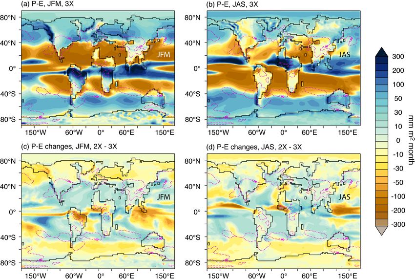
342                                                     A. Toumoulin et al.: Evolution of continental temperature seasonality

This event is associated with the first major expansion           and highest temperatures within a year. This is the case for
of the Antarctic ice sheet with an estimated sea-level            the Climate Leaf Analysis Multivariate Program (CLAMP),
drop of ∼ 70 m (Hutchinson et al., 2021; Miller et al.,           which reconstructs temperatures from the modern correla-
2020). The EOT is described as a relatively brief event           tion between climate variables and leaf physiognomy (Wolfe,
(∼ 790 000 years), with two successive steps (at ca. 33.9         1993; Yang et al., 2011), or the Coexistence Approach (CA),
and 33.7) recognized in extensively studied marine environ-       which uses modern relatives of fossil species to define a mu-
ments, especially from deep ocean δ 18 O values (e.g., Katz et    tual climate range of environmental characteristics (Grimm
al., 2008; Zachos et al., 2001; see the review of Hutchinson      and Potts, 2016; Mosbrugger and Utescher, 1997; Utescher
et al., 2021).                                                    et al., 2014). MATR can also be deduced from the variability
   Reported vegetation responses to the EOT appear to be          of the temperature signal in geochemical proxies for temper-
heterogeneous across continents with important composition        atures, stable oxygen isotopes (δ 18 O), as the time resolution
changes in some areas (e.g., the west coast of the United         of the proxy rarely allows for the direct reconstruction of
States, Greenland, Asia), notably where faunal turnover is        seasonal temperatures (e.g., Ivany et al., 2000; Wade et al.,
important (e.g., Barbolini et al., 2020; Hutchinson et al.,       2012).
2021; Pound and Salzmann, 2017; Wolfe, 1994). A num-                 The spatial distribution of temperature seasonality changes
ber of paleobotanical and geochemical studies consistently        across the EOT appears to be heterogeneous in proxy data
suggest that the decrease in continental temperatures was         (e.g., Pound and Salzmann, 2017). Most changes are de-
particularly marked during winter months, thus leading to         scribed in the Northern Hemisphere from paleobotanical re-
higher seasonal temperature contrasts, which are designated       constructions and converge to show seasonalities stronger
as a potential driving mechanism for biotic turnovers (e.g.,      in the early Oligocene than in the mid- to late Eocene.
Eldrett et al., 2009; Mosbrugger et al., 2005; Page et al.,       In North America, western and central Europe, seasonal-
2020; Utescher et al., 2015; Zanazzi et al., 2015). Evoked        ity increase is recorded by the decline in species character-
forcing mechanisms explaining this enhanced winter cooling        istic of warm paratropical to temperate environments such
are pCO2 , Antarctic ice-sheet (AIS) inception and increased      as palms (e.g., Nypa sp.), plants from the myrtle and eu-
continentality, although it remains difficult to quantify and     calyptus family (Myrtaceae, e.g., Rhodomyrtophyllum sp.),
disentangle their respective contribution from field data only.   conifers (e.g., Doliostrobus sp.) and some plant families with
Understanding the drivers of these seasonal changes is thus       tropical elements (e.g., Annonaceae, Lauraceae, Cornaceae,
important, not only for assessing the climate system behav-       Icacinaceae, Menispermaceae), and, depending on the bio-
ior under major pCO2 variations but also to better describe       climatic zones, the expansion of temperate to boreal vege-
the paleoenvironmental context associated with major extinc-      tation through the increase in deciduous and/or coniferous
tion events of the EOT such as the Grande Coupure in Eu-          species (Kunzmann et al., 2016; Kvaček, 2010; Kvaček et
rope and the Mongolian Remodeling in central Asia (Meng           al., 2014; Mosbrugger et al., 2005; Utescher et al., 2015;
and McKenna, 1998; Stehlin, 1909; see Coxall and Pearson,         Wolfe, 1992). These vegetation changes are associated with
2007, for a review).                                              a decrease in the coldest month mean temperature (CMMT)
   By comparing paleoclimate simulations to a synthesis of        across the EOT and start before the EOT at some locali-
indicators of seasonality changes (Table S1 in the Supple-        ties, during the mid- to late Eocene (Moraweck et al., 2019;
ment), our study attempts to retrieve the evolution of seasonal   Mosbrugger et al., 2005; Tanrattana et al., 2020; Tosal et al.,
temperature contrast from the middle Eocene to the early          2019; Utescher et al., 2015; Wolfe, 1994). Isotopic analyses
Oligocene. The EOT is reconstructed step by step from five        have documented this seasonality increase in different con-
simulations, describing the evolution of three major forcings     tinental localities between the Priabonian (37.8 to 33.9 Ma)
of this time: the pCO2 drawdown, the AIS expansion and            and the Rupelian (33.9 to 27.82 Ma; Grimes et al., 2005;
the resulting sea-level lowering, in order to understand the      Hren et al., 2013; Zanazzi et al., 2015). While some of the
respective contribution of each component to the resulting        changes are not directly quantifiable (e.g., the reduction in
seasonality change patterns, along with their possible syner-     gastropod growing season length, United Kingdom; Hren et
gies and retroactions.                                            al., 2013; dental morphological changes for grazing perisso-
                                                                  dactyls, Europe; Joomun et al., 2010), others can demonstrate
1.2   Temperature seasonality and its evolution
                                                                  strong MATR increase (e.g., amplified by 15.6 ◦ C, Canada;
                                                                  Zanazzi et al., 2015). A temperature seasonality increase is
Temperature seasonality can be quantified by the mean an-         also documented for shallow waters of the Gulf of Mexico
nual temperature range (MATR), which consists of the tem-         (increase in the MATR; Ivany et al., 2000; Wade et al., 2012).
perature difference between the warmest and coldest months        Some studies have suggested a link between increased tem-
of the year. Increasing MATR can occur through increased          perature seasonality and latitude (e.g., Zanazzi et al., 2007,
summer temperatures, lowered winter temperatures or both.         2015), but data seem insufficient to validate this relationship,
MATR is practical because it can be directly calculated from      and this trend has not been confirmed by recent palynological
temperature proxies providing an estimation of the lowest         compilation (Pound and Salzmann, 2017).

Clim. Past, 18, 341–362, 2022                                                         https://doi.org/10.5194/cp-18-341-2022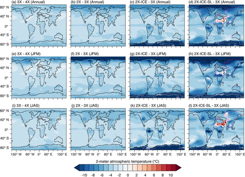
A. Toumoulin et al.: Evolution of continental temperature seasonality                                                      343

   Data from southeast Europe and Anatolia show generally         from 910 to 560 ppm (i.e., a drop of 1.6X). In addition,
weaker and heterogeneous changes in temperature season-           a recent model–data study of Lauretano et al. (2021) ex-
ality, with either no seasonality changes, slight seasonality     plored Australia climate evolution through the EOT, and es-
lowering or slight seasonality strengthening from the mid-        timated a pCO2 drop ranging from 260 to 380 ppm (drop
Eocene to the Rupelian (Bozukov et al., 2009; Kayseri-Özer,       of ∼ 0.9–1.3X). A first attempt to explain temperature sea-
2013). This variability has been explained by a strong ma-        sonality change across the EOT was made by Eldrett et
rine influence on this part of Eocene Europe (Kayseri-Özer,       al. (2009). In their palynological and modeling study, Eldrett
2013). Conversely, north and East Asia temperature season-        and coauthors explained high-latitude (Greenland) seasonal-
ality evolution is more comparable to western Europe and          ity strengthening by pCO2 drop and the consequent increase
North America trends (Quan et al., 2012; Utescher et al.,         in sea-ice formation over the Arctic Ocean. In their exper-
2015). Vegetation changes reflect an increase in the seasonal     iment, sea-ice extension induces a strong albedo feedback,
temperature range, mainly through the EOT (MATR increase          which results in a large decrease in atmospheric tempera-
of 2 to 2.5 ◦ C; CMMT decrease of ∼ 2.2 ◦ C, Quan et al.,         ture during winter. Additionally, changes in geography (to-
2012; Utescher et al., 2015). The appearance of tubers in         pography, land–sea distribution) may have significant effects
lotus (Nelumbo sp.) during the Eocene suggests the estab-         on terrestrial temperatures at a regional scale (e.g., Lunt et
lishment of a dormant phase in these plants and thus of a         al., 2016; Li et al., 2018). EOT modeling experiments yield
period unfavorable to plant growth (Li et al., 2014). Fos-        mixed answers regarding the temperature feedback resulting
sils showing these structures have been described in south-       from both AIS and contemporary paleogeographic changes
ern China (Hainan Province) and easternmost Russia (Kam-          (opening of Southern Ocean gateways, Antarctic geography
chatka Peninsula) leading to the hypothesis that they could       or global geography; Goldner et al., 2014; Hutchinson et al.,
be favored by cooling and increased seasonality on the East       2021; Kennedy et al., 2015; Ladant et al., 2014a, b). The few
Asian continent during the Eocene (Budantsev, 1997; Li et         studies testing the combined effect of both AIS and paleo-
al., 2014).                                                       geographic changes (Kennedy et al., 2015; Lauretano et al.,
   In the Southern Hemisphere, studies of Paleogene locali-       2021) suggested a moderate impact of AIS on global climate
ties are rarer. Despite a record of late Eocene cooling in Aus-   sensitivity, as previously suggested by other modeling work
tralia, New Zealand and Patagonia, independent proxies (sta-      (Goldner et al., 2013; Kennedy et al., 2015).
ble isotopes on teeth, bones and pedogenic carbonates, pa-
leobotanical reconstructions) do not suggest a marked tem-
                                                                  2     Material and methods
perature seasonality during the Eocene (Colwyn and Hren,
2019; Kohn et al., 2015; Lauretano et al., 2021; Nott and         2.1    Model and simulation setting
Owen, 1992; Pocknall, 1989). In Australia, the presence of
more pronounced tree rings suggests a late Paleogene in-          We used the IPSL-CM5A2 general circulation model, which
crease in seasonality starting in the mid-Oligocene at the ear-   is built upon the CMIP5 Earth system model developed at
liest (Bishop and Bamber, 1985; Nott and Owen, 1992). Fi-         the Institut Pierre-Simon Laplace (IPSL), i.e., IPSL-CM5A-
nally, the environmental and climatic impact of the EOT in        LR (Dufresne et al., 2013; Sepulchre et al., 2020). The IPSL-
continental Africa remains poorly documented (Hutchinson          CM5A-LR Earth system model is composed of the LMDZ
et al., 2021; Saarinen et al., 2020).                             atmospheric model (Hourdin et al., 2013), the ORCHIDEE
                                                                  land surface and vegetation model (Krinner et al., 2005),
1.3   Previous model work
                                                                  and the NEMO v3.6 ocean model which includes modules
                                                                  for ocean dynamics (OPA8.2; Madec, 2016), biochemistry
Different modeling studies have illustrated the priming role      (PISCES; Aumont et al., 2015) and sea ice (LIM2; Fichefet
of pCO2 lowering during the EOT, but most focused on              and Morales-Maqueda, 1997). The atmospheric grid has a
oceans through mean annual temperature changes (Baat-             horizontal resolution of 3.75◦ longitude per 1.875◦ latitude
sen et al., 2020; Goldner et al., 2014; Hutchinson et al.,        (96 × 95 grid points) and is divided into 39 vertical levels.
2018, 2021; Kennedy et al., 2015; Kennedy-Asser et al.,           For a more detailed description of the model and its different
2019, 2020; Ladant et al., 2014b). The model intercompar-         components, the reader is referred to Sepulchre et al. (2020).
ison study of Hutchinson et al. (2021) has shown a reason-           Five simulations were carried out to reconstruct the evo-
able agreement between modeling experiments with 1120             lution of temperature seasonality from the middle Eocene
and 560 ppm (i.e., 4 and 2 times the preindustrial atmo-          to the early Oligocene (Table 1). The applied 40 Ma pa-
spheric levels, respectively, with 1 PAL = 280 ppm and here-      leogeography framework is the map developed by Poblete
after written “4X” and “2X”) and proxy-data atmospheric           et al. (2021) and already used in Tardif et al. (2020) and
and surface ocean temperature reconstructions from the late       Toumoulin et al. (2020). It features common late Eocene ge-
Eocene and the early Oligocene, respectively. They show,          ography characteristics such as an open Panama Seaway, an
however, that changes in EOT sea surface temperatures             open Tethys with a submerged Arabian Peninsula, a strongly
(SSTs) were on average best represented by a pCO2 shift           maritime Europe, a Turgai land bridge connecting north-

https://doi.org/10.5194/cp-18-341-2022                                                         Clim. Past, 18, 341–362, 2022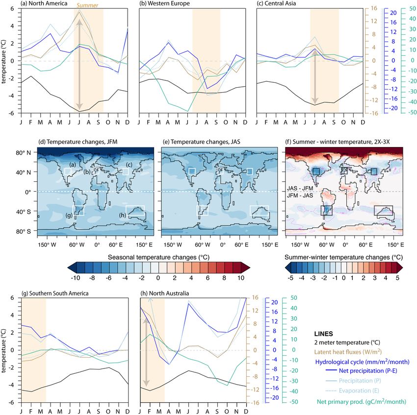
344                                                     A. Toumoulin et al.: Evolution of continental temperature seasonality

ern Europe with Asia and narrow Southern Ocean gateways           the long-term cooling of the Eocene. The inclusion of data
(Fig. 1). The orbital parameters were set to preindustrial val-   from the middle Eocene allows a comparison with simula-
ues and the solar constant was reduced accordingly to its         tions testing the effect of a pCO2 lowering alone, before AIS
Eocene value (1360.19 W m−2 ; Gough, 1981). Vegetation            formation at the EOT. It is justified by the presence of pa-
was implemented as a boundary condition, using a zonal            leobotanical records suggesting a strengthening of the sea-
band of PFTs using modern vegetation distribution patterns.       sons already from the Lutetian to the Priabonian (e.g., Li
   Simulations were compared in pairs to highlight dif-           et al., 2014; Mosbrugger et al., 2005). Compiled Eocene–
ferences between the middle/late Eocene and the early             Oligocene 1MATRs correspond either to the values given in
Oligocene. The simulation set is composed of both realis-         original publications, when they were available and precise,
tic and idealized experiments (Table 1). Simulations 4X, 3X       or to values recalculated from the original data. For publica-
and 2X represent most of the pCO2 range described from            tions for which 1MATRs were recalculated, we proceeded
the mid-Eocene (Lutetian) to the early Oligocene (Rupelian;       by grouping the closest sites (especially in terms of latitudes)
Foster et al., 2017). These pCO2 values enable the descrip-       and checked that the values obtained were consistent with
tion of the pCO2 reduction effect on climate through this         the authors’ original interpretation of the paleoenvironmental
time interval and have been used in most previous modeling        context. Half of the data come from the pollen compilation of
experiments on the EOT (Hutchinson et al., 2021). Simula-         Pound and Salzmann (2017). A selection was made through
tions 4X and 3X cover the range of potential climate val-         this study data to keep (1) the best-dated samples, according
ues prior to the EOT (Lutetian to Priabonian). The ideal-         to their dating quality indicator (data Q1 to Q3; Pound and
ized simulation 2X allows the identification of a 1 to 2 PAL      Salzmann, 2017), and (2) sites with temperature estimates
pCO2 lowering alone. In a complementary way, simulations          for the Priabonian and Rupelian or at least one nearby local-
2X-ICE and 2X-ICE-SL describe the early Oligocene cli-            ity that could be compared. No Eocene–Oligocene site was
mate, following the Antarctic ice-sheet formation. Both sim-      selected for more clarity. In an effort to limit the addition of
ulations are parameterized in the same way apart from the         overly uncertain 1MATR data, sites with a range of CMMT
sea level, which is 70 m lower in 2X-ICE-SL. The use of           estimates (CMMTmax –CMMTmin ) ≥ 10 ◦ C (either for Pri-
2X-ICE provides a theoretical description of the effect of an     abonian or Rupelian sites) were excluded.
ice-covered Antarctica on climate, while 2X-ICE-SL consti-           Some previously published seasonality increases were not
tutes a more realistic representation of the early Oligocene      associated with estimates of 1MATR because seasonality
climate. In these experiments, the Antarctic ice cap was set      strengthening was either (1) suggested from other parame-
to 32.5 × 10⁶ km3 according to Ladant et al. (2014b). The         ters, such as the length of the growing season, which does
70 m sea-level drop was defined following eustatic drop es-       not allow the calculation of the MATR (Hren et al., 2013),
timates for the EOT (Coxall et al., 2005; Katz et al., 2008;      or (2) derived from qualitative data that cannot be specifi-
Lear et al., 2008; Miller et al., 2020). It is responsible for    cally associated with temperature values (e.g., morpholog-
important geography changes related to an increase in land        ical changes such as tooth shape or plant tuber appearance;
proportion, such as the emergence of the Arabian Peninsula        Joomun et al., 2010; Li et al., 2014). These sites are displayed
and the retreat of the proto-Paratethys epicontinental sea.       on the maps in orange but are not included in quantitative
   All simulations run for 4000 years until temperatures in-      analyses (Sect. 2.3). In order to better estimate the impact of
dicate a quasi-equilibrium with only negligible temperature       changes in temperature seasonality, the length of the plant
drift within the global mean ocean (< 0.1 ◦ C per century;        growing season (i.e., the number of months with an average
Fig. S1 in the Supplement). These trends are consistent with      temperature above 10 ◦ C) was recalculated using the formula
most model studies and do not affect the quality of atmo-         of Grein et al. (2013) for Coexistence Approach data (Ta-
spheric change described in this study (e.g., Hutchinson et       ble 1). Paleocoordinates for every locality were reconstructed
al., 2018; Lunt et al., 2016). The results considered here are    using the online service of Gplates (https://www.gplates.org/,
averages of the last 100 years of the model runs.                 last access: 16 February 2022), according to the 40 Ma pale-
                                                                  ogeography used for the paleoclimate models (Poblete et al.,
2.2   Data compilation
                                                                  2021) that essentially follows the plate tectonic reconstruc-
                                                                  tion model of Matthews et al. (2016) with some modifica-
Simulation results were compared to MATR changes                  tions.
(1MATR) documented by proxy-data records (Table S1 in
the Supplement). We compiled published MATR and CMMT              2.3   Comparison of model and data ∆MATR
proxy data from various research fields: paleobotany (macro-
fossils and palynology), geochemistry (isotopic measure-          Different analyses were made to evaluate the data–model
ments on various material) and paleontology. The data were        agreement for temperature seasonality changes from the Pri-
selected to range from the Lutetian (47.8 Ma) to the end of       abonian to Rupelian (Table 2). Modeled 1MATR values
the Rupelian (27.8 Ma). This large time interval allows the       were extracted from a 3◦ longitude by 3◦ latitude area sur-
representation of seasonal temperature changes parallel to        rounding each data locality. First, a general agreement per-

Clim. Past, 18, 341–362, 2022                                                         https://doi.org/10.5194/cp-18-341-2022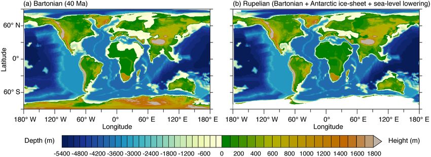
A. Toumoulin et al.: Evolution of continental temperature seasonality                                                                 345

Table 1. Experimental design. Abbreviations: AIS – Antarctic ice-sheet volume (Ladant et al., 2014b); %Land – total land surface (millions
of square kilometers – 106 km2 ); MAT – mean annual global 2 m air temperature (◦ C); SST – sea surface temperature (◦ C). Simulations with
an asterisk constitute realistic middle Eocene (Lutetian/Bartonian) and early Oligocene (Rupelian) scenarios; others are either sensitivity
experiments (2X, 2X-ICE) or use the high value of the pCO2 range estimated for the time interval (4X).

                        Simulation         pCO2            AIS          %Land (Mkm2 )      MAT (◦ C)     SST (◦ C)
                        4X              1120 ppm            –                132.3            26.4         28.2
                        3X ∗             840 ppm            –                132.3            23.7         25.9
                        2X               560 ppm            –                132.3            20.6         23.2
                        2X-ICE           560 ppm     32.5 × 10⁶ km3          132.3            19.7         22.9
                        2X-ICE-SL∗       560 ppm     32.5 × 10⁶ km3          152.7            18.7         22.2

Figure 1. Paleotopographic 40 Ma map: (a) standard version as used for simulations 4X, 3X, 2X and 2X-ICE; (b) version adjusted with a
homogeneous 70 m sea-level lowering used for the simulation 2X-ICE-SL (Poblete et al., 2021).

centage was calculated from the direction of seasonality                of the method). Conversely to the Spearman rank test, for
changes alone to assert the agreement between our simula-               which mean 1MATR estimations were used, the distance
tion and qualitative data. For this metric, model predictions           is here measured using the full range of estimates at each
are considered “good” for an individual site if the modeled             data locality (i.e., minimum and maximum 1MATR). Note
1MATR changes in the same direction as the data (i.e., if               that, because it considers the full range of 1MATR, this
a modeled 1MATR increases/decreases at the location of a                method tends to minimize the difference between model and
data point showing seasonality increase/decrease). For data             data. The lower bound of modeled 1MATR at each locality
indicating null 1MATR, good agreement was considered to                 was calculated as the difference between the lowest MATR
exist when model values ranged from −0.5 to 0.5 ◦ C.                    value over the 3◦ × 3◦ area centered around the locality for
   In addition, Priabonian to Rupelian seasonality changes              an Oligocene-like cold simulation (2X, 2X-ICE or 2X-ICE-
were compared to model predictions, by (1) testing their cor-           SL) and the highest MATR value over the 3◦ × 3◦ area for
relation and (2) calculating the root of the mean squared dis-          an Eocene simulation (4X or 3X). For the upper bound, we
tance between their values. These two analyses were per-                used the difference between the higher MATR value over
formed using R (version 4.0.3; R CoreTeam, 2020, Boston,                the same area for an Oligocene-like cold simulation and the
USA). Given the limited number of quantitative Priabonian–              lower MATR value for an Eocene simulation.
Rupelian data (n = 29), the statistical correlation of data–               The RMSE adjusted to 1MATR is written as follows:
model 1MATR was assessed from average 1MATR with
                                                                        RMSE(1MATR) =
the non-parametric Spearman rank test. In this analysis, we                 v
used the common significance level, α, of 0.05 (i.e., p val-                uX 1MATR(data) − 1MATR(model) 2
                                                                            u n
ues < 0.05 indicate significant correlations). The root mean                t                               ,                          (1)
                                                                                            n
squared estimate consists of calculating the root of the mean                 i=1
squared distance between model and data values for com-                 where 1MATRdata and 1MATRmodel are MATR Priabonian
parable points (RMSE; see Kennedy-Asser et al., 2020, and               to Rupelian changes estimated by data and model, respec-
their Fig. S1 in the Supplement for a detailed presentation             tively, and n is the total number of localities.

https://doi.org/10.5194/cp-18-341-2022                                                                 Clim. Past, 18, 341–362, 2022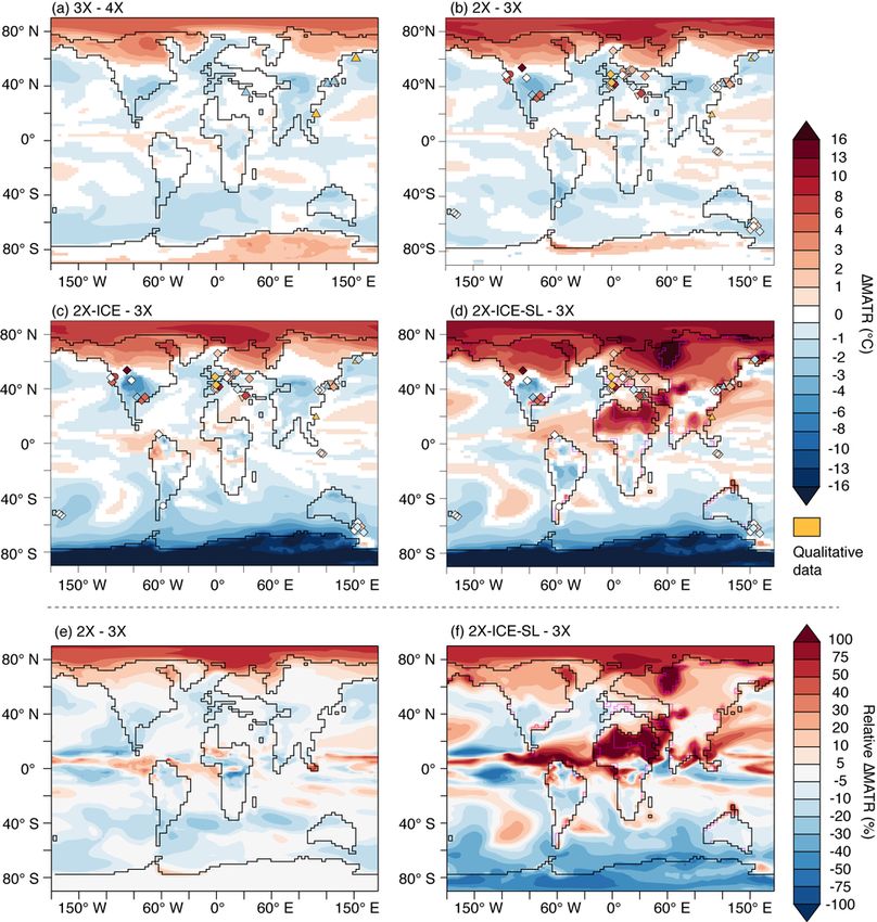
346                                                        A. Toumoulin et al.: Evolution of continental temperature seasonality

3     Results                                                        3.1.2   Areas with decreased seasonality

3.1     Simulated response to pCO2 lowering                          Areas with decreased seasonality are characterized by sum-
                                                                     mer cooling that exceeds winter cooling, which reduces the
In this section, we compare the simulations 4X, 3X and
                                                                     MATR (Figs. 2 and 4). The widest zones of decreasing
2X together to describe the effects of pCO2 drawdown on
                                                                     MATR are continental regions located within the 30–50◦ lat-
climate and provide a range of possible MAT and MATR
                                                                     itudinal band. The magnitude of simulated MATR reduction
change intensities. The simulation pair 2X–4X represents the
                                                                     depends on the pCO2 drop considered, with a reduction from
strongest possible changes, 3X–4X the weakest changes and
                                                                     3X to 2X and from 4X to 2X resulting in up to 20 % and
2X–3X an intermediate scenario (see Sect. 2.1). Mean an-
                                                                     30 % of regional MATR decrease, respectively (Figs. 4 and
nual temperatures decrease strongly in our different experi-
                                                                     S3). At lower latitudes, in Amazonia, equatorial Africa and
ments (Table 1, Fig. 2). The halving of pCO2 from 4X to
                                                                     India, seasonality decreases but to a lesser extent (Fig. 4).
2X alone (i.e., without AIS formation and sea-level drop)
                                                                     A variety of atmospheric and oceanic processes are likely in-
induces a global cooling of 5.8 and 5.0 ◦ C for the air temper-
                                                                     volved in these contrasting MATR changes, depending on the
ature and the surface ocean, respectively (Table 1). A pCO2
                                                                     region considered.
drop of 1 PAL induces a 2.7 to 3.1 ◦ C lowering of MAT and
                                                                        The good correlation between MATR increase (respec-
a 2.3 to 2.7 ◦ C cooling of the SST, for 4X to 3X and 3X
                                                                     tively, decrease) and net precipitation decrease (respectively,
to 2X changes, respectively. Along with its effect on annual
                                                                     increase; i.e., North America, Central Asia and northern Aus-
temperatures and regardless of its intensity, pCO2 decrease
                                                                     tralia) suggests a strong involvement of the hydrological cy-
induces zonal 1MATR including (1) an increase in MATR
                                                                     cle in this phenomenon (Figs. 5 and 6a, c and h). The pCO2
at high latitudes (especially in the north), (2) a decrease in
                                                                     drop tends to slow down the hydrological cycle, which re-
MATR across most midlatitudes and (3) moderate changes
                                                                     sults in flatter latitudinal gradients. At high latitudes, a re-
at low latitudes, which we detail in the following Sects. 3.1.2
                                                                     duction in precipitation leads to an overall decrease, while at
and 3.1.3 (for Eocene MATR values, see Fig. S2).
                                                                     midlatitudes to low latitudes, increased precipitation results
                                                                     in a general increase (Figs. 5 and 6). In these low-latitude
3.1.1    Areas with increased seasonality                            to midlatitude zones, precipitation strengthening is more im-
Temperature changes are characterized by polar amplifica-            portant in summer and associated with increased evapora-
tion, with a stronger winter cooling at high latitudes (Fig. 2a,     tion, which results in larger latent heat fluxes and thus in a
b, e, f, i and j), likely due to the combined effect of albedo and   greater cooling during summer, consistently with decreased
sea-ice feedback. Below a given threshold (situated between          seasonality (Fig. 6a, c, h). In addition, summer cooling is
2 and 3 PAL), the pCO2 drop enables sea-ice growth over the          strengthened through vegetation feedback: increase favors
Arctic and, to a lesser extent, the subsistence of snow on the       net primary productivity which in turn contributes to evap-
ground during the cold season, which increases winter sur-           oration and summer warmth loss (Fig. 6a, c, h). In contrast,
face albedo (Fig. 3). In addition, seasonal sea-ice expansion        decreased MATR in Europe and southern South America ap-
limits ocean-to-air heat transfer at the highest northern lati-      pears poorly correlated to the above-mentioned parameters
tudes and contributes to further winter cooling of the atmo-         (Fig. 6b and g). For Europe, the presence of sea ice over
sphere. This preferential lowering of winter temperatures re-        the Arctic Ocean (Fig. 3b–e) limits heat loss via the atmo-
sults in a large MATR increase of 5–20 % (3X–4X and 2X–              sphere during winter and results in a greater summer cool-
3X) and up to 40 % (2X–4X; Figs. 4e and S3b) over high               ing of the SST (Fig. S5), which contributes to lowering Eu-
northern latitudes. Furthermore, the areas of colder winters         ropean MATR. In addition, a regional increase in low-level
and high MATR widen as pCO2 decreases: MATR increases                cloud cover during summer could also contribute to lowering
from 60◦ N poleward between 4X and 3X, to 50◦ N poleward             MATR for both Europe and southern South America through
between 4X and 2X (Figs. 4 and S4). In contrast, Antarctica          albedo feedback (5 % to 15 % higher low-level cloud fraction
shows moderate 1MATR (regionally up to 3 ◦ C from 4X to              between 40–60◦ ; Figs. 7 and S6). For southern South Amer-
3X and 6 ◦ C from 3X to 2X) compared to high northern lat-           ica, several parameters seem consistent with the MATR re-
itude lands (6 ◦ C MATR increase from 4X to 3X and 10 ◦ C            duction, but it is difficult to disentangle their contribution. By
from 3X to 2X). This is because Antarctica is characterized          amplifying the latitudinal temperature gradients, the pCO2
by high MATR values in all ice-sheet-free experiments (4X,           drop induces a northward migration of the westerly wind
3X and 2X), resulting in low 1MATR changes from one ex-              maximum (by about 2◦ of latitude annually but less markedly
periment to another (Fig. 4a and b). This important seasonal-        during austral winter, JAS) and of the Antarctic Circumpolar
ity is induced by the continent’s high albedo variability, as it     Current, which delimits the Southern Hemisphere subpolar
oscillates from snow-free to snow-covered soil within a year.        and subtropical gyres. This northward shift limits the arrival
                                                                     of warm subtropical waters near the poles (Fig. S7). This
                                                                     greater cooling in summer SST reinforces the ocean’s buffer-
                                                                     ing effect on atmospheric temperatures in southern South

Clim. Past, 18, 341–362, 2022                                                             https://doi.org/10.5194/cp-18-341-2022
A. Toumoulin et al.: Evolution of continental temperature seasonality                                                                        347

Figure 2. Two-meter air temperature changes ( ◦ C). JFM: averaged over January to March; JAS: averaged over July to September. Magenta
lines of (d), (h) and (l) indicate shorelines before sea-level lowering. White dotted lines in (c), (d), (g), (h), (k) and (l) are the level lines
encircling the 20, 40 and 45 ◦ C cooling zones.

Figure 3. Northern Hemisphere winter sea-ice fraction and surface albedo (%).

https://doi.org/10.5194/cp-18-341-2022                                                                       Clim. Past, 18, 341–362, 2022

348                                                         A. Toumoulin et al.: Evolution of continental temperature seasonality

Figure 4. Changes in mean annual temperature range, 1MATR (◦ C). Shadings are model differences calculated with a Student t test over the
last 100 years of comparative simulations (95 % confidence); white areas indicate no significant 1MATR. Panels (e) and (f) indicate relative
1MATR (in %) for 2X–3X and 2X-ICE-SL–3X, respectively. Symbols correspond to 1MATR from proxy data for different time steps:
Priabonian–Lutetian (triangles); Rupelian–Lutetian (inverted triangles); Rupelian–Bartonian (circles); Rupelian–Priabonian (diamonds). Or-
ange symbols indicate qualitative values describing a temperature seasonality increase. In the case of proxies reconstructing a range of
equally probable values (e.g., the Coexistence Approach), the values shown are mean values. References are displayed in Fig. 8 and available
in the data compilation provided in Table S1 in the Supplement.

America and favors milder summers, and to a lesser extent,              3.2     Modeled response to Antarctic ice sheet and
cooler winters, which is consistent with a decrease in season-                  sea-level drop
ality (Figs. 4 and 7). Finally, changes in atmospheric dynam-
ics (decrease in the width and increase in the intensity of the         3.2.1    Antarctic ice sheet only
Hadley cell) are also visible and could have an impact on air–          AIS formation is responsible for a supplementary 0.9 and
ocean exchanges, but much more analysis would be needed                 0.3 ◦ C cooling of the air temperature and the surface ocean,
to understand their implication, which is not the focus of this         respectively (Table 1). Its direct effect on 2 m mean an-
paper (Fig. S8).                                                        nual temperatures varies regionally and is more striking over
                                                                        Antarctica with up to −35 ◦ C cooling and over the Southern
                                                                        Ocean and Australia (Figs. 2c, g, k and S3c and d). In contrast
                                                                        with Arctic sea ice which increases seasonality at the highest
                                                                        northern latitudes, the AIS decreases southern latitude tem-
                                                                        perature seasonality (Figs. 4c and S3c and d). Indeed, simu-

Clim. Past, 18, 341–362, 2022                                                                 https://doi.org/10.5194/cp-18-341-2022
A. Toumoulin et al.: Evolution of continental temperature seasonality 349
Figure 5. Net precipitation (precipitation − evaporation) in JAS and JFM for the late Eocene simulation 3X (a, b). Changes associated with
pCO2 drop from 3X to 2X (differences shown are 2X−3X) for net precipitation (c, d). Magenta dashed lines contour areas with decreased
seasonality (1MATR ≤ −1 ◦ C) in 2X−3X simulations (blue zones in Fig. 4b).
lations with the AIS have a yearlong white Antarctica with platform and the modification of the East Asian coastlines
high and stable albedo, which reduces seasonal temperature (Figs. 4d and S3e and f).
variability (Fig. 3g–l).
3.3 Model–data comparison
3.2.2 Sea-level drop 3.3.1 pCO2 lowering
Sea-level decrease alone is responsible for a 1.0 ◦ C
cooling The 1MATR described by the pCO2 drop experiments (from
of global MAT (0.7 ◦ C for surface oceans) and results in con- 3X or 4X to 2X) show no good agreement either with mid-
siderable regional temperature changes in areas with impor- dle to late Eocene or with late Eocene to early Oligocene data
tant land–sea distribution changes (Table 1, Figs. 4d and f estimates (Figs. 4a and b and 8b). The simulations predict no
and S3e and f). The marine regions that become exposed af- change, or a MATR decrease, in areas where the Lutetian–
ter sea-level drop show the strongest increase in MATR, as Priabonian data points (n = 6, triangles, Fig. 4a) describe
they experience both winter cooling and summer warming, increased seasonality (Fig. 4a and b). Priabonian–Rupelian
due to the lower thermal inertia of land compared to ocean. 1MATR modeled through 4X to 2X and 3X to 2X pCO2
This seasonality strengthening in newly exposed areas oc- drops is, on average, lower than data estimates at similar lo-
curs independently of their latitude, therefore disrupting the calities, with a mean offset of −3.5 and −2.8 ◦ C, respectively
otherwise zonal distribution of seasonal temperature changes (Fig. 8b; Table 2). The use of the simulation 4X instead of
generated by pCO2 drop and AIS formation (Figs. 4f and 3X for the late Eocene stage has a marginal effect on the per-
S3f). The effect on seasonality of these disappearing seas ex- centage of agreement for the sign of the 1MATR, although a
pands beyond areas adjoining the emerging landmasses due slightly higher value is observed for 3X–2X (Table 2, line
to the resulting regional perturbation in temperature. North- “%”, Figs. 8b and S9). In addition, the pCO2 drop alone
ern Africa, western Asia and Russia are the most impacted leads to zonal 1MATRs which do not transcribe the spatial
areas, due to the retreat of the proto-Paratethys sea and the heterogeneity visible in data. This misfit is visible through
emergence of the Arabian Peninsula (Fig. 1). More moder- high RMSE scores and the absence of significant correlation
ate seasonality changes are also visible as a result of sea re- between modeled 1MATR resulting from the pCO2 drop
treats of smaller extent, such as the emergence of the Florida (simulations 2X–4X and 2X–3X) and 1MATR described by
https://doi.org/10.5194/cp-18-341-2022 Clim. Past, 18, 341–362, 2022350 A. Toumoulin et al.: Evolution of continental temperature seasonality
Figure 6. Annual variability of multiple climate parameters within the different areas of decreasing seasonality between 3X and
2X (a–c, g, h): atmospheric temperature (black), latent heat fluxes (soil to atmosphere; brown), hydrological cycle (including precipitation,
evaporation and net precipitation; different shades of blue) and net primary productivity (green). Temperature changes and summer−winter
temperature changes (d–f). Rectangles outline the land areas analyzed in (a)–(c), (g) and (h) (ocean zones are not taken into account in the
calculation of the plots). Gray arrows show where decreasing summer temperatures match increased latent heat fluxes.
proxy data (Table 2). Two data–model agreement patterns are 3.3.2 Antarctic ice sheet and sea level
nevertheless to be noted: (1) regardless of their values (which
The formation of the AIS alone does not result in a bet-
are higher in data than in our simulations), the northernmost
ter agreement between modeled and Priabonian–Rupelian
data points are inside or surround the high-latitude seasonal-
1MATR estimates. It is even slightly reduced (Table 2). The
ity strengthening zone we modeled (Fig. 4, data points 1, 2
reinforcement of the MATR lowering zone at high south-
and 3 in Fig. 8a); (2) none of the Southern Hemisphere data
ern latitudes increases the data–model misfit because of data
localities showing no seasonality change are located within
points indicating null 1MATR in this zone (Figs. 4c and
MATR increase zones (Fig. 4b).
8b). There is still no significant correlation between 1MATR
from the model and differences documented by proxy data
(Table 2).
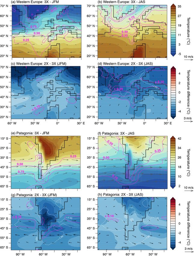
Clim. Past, 18, 341–362, 2022 https://doi.org/10.5194/cp-18-341-2022A. Toumoulin et al.: Evolution of continental temperature seasonality 351 Figure 7. Two-meter atmospheric temperature across western Europe and Patagonia. Shadings correspond to temperatures (a, b, e, f) and temperature differences (c, d, g, h). Similarly, magenta lines contour low-level fraction (a, b, e, f) and low-level cloud fraction changes (c, d, g, h; always expressed in %) and arrows, 850 hPa winds (a, b, e, f) and 850 hPa wind changes (c, d, g, h; always in m s−1 ). White dashed lines contour areas with decreased seasonality (1MATR ≤ −1 ◦ C) in 2X−3X simulations (blue zones in Fig. 4b). Geographic changes associated with sea-level drop result regions directly impacted by the sea-level drop, as for ex- in a better agreement with data 1MATR (Figs. 4d and 8b). ample data estimates located on the Pacific Coast (Fig. 4d). The largest continental fraction changes affect the MATR Similarly, coastline changes along the eastern part of Africa on a broad geographic scale and allow for a better agree- and western Asia cause an increase in seasonality in Anatolia ment, even with several data points standing away from the and central/western Europe, improving the fit between model https://doi.org/10.5194/cp-18-341-2022 Clim. Past, 18, 341–362, 2022
352                                                            A. Toumoulin et al.: Evolution of continental temperature seasonality

Figure 8. Data–model comparison of 1MATR from the Priabonian to the Rupelian. (a) Map of all data 1MATR estimates compiled in
this study (symbols refer to the time period compared for the calculation of the MATR shift; see Table S1 in the Supplement for associated
references). The points marked with an asterisk have an uncertain origin (marine sediments) and have not been taken into account in the
statistical analyses although they are shown here. The points marked with an asterisk have an uncertain origin (marine sediments) and have
not been taken into account in the statistical analyses although they are shown here. (b) Comparison of data estimates of Priabonian–Rupelian
1MATR (black diamonds) to modeled 1MATR at the same localities (colored circles, calculated over a 3 × 3◦ area) from different pairs of
simulations with 3X. Error bars are minimum and maximum data estimates of 1MATR. The dashed black line is the LOESS curve associated
with data 1MATR estimates. Bold colored lines indicate the continental latitudinal gradient of 1MATR on land (i.e., all longitudes averaged
per degree of latitude); color-shaded intervals are the standard deviation around the average. A subfigure similar to (b) but using the simulation
4X as a Priabonian stage is available in the Supplement, Fig. S9.

and data. These changes in temperature seasonality result in               along the East Asian coast increase seasonality at a regional
a reduction of 2 to 2.5 months in the duration of the plant                scale and improve the data–model fit (data points 14, 22 and
growing season (as reconstructed with the formula of Grein                 24). This better fit is transcribed through the RMSE analysis
et al., 2013; Table S1 in the Supplement). Smaller changes                 results, the lowest values being obtained when the simula-
in coastlines such as in Florida, the Kamchatka Peninsula or               tion 2X-ICE-SL is used to simulate the Rupelian stage (Ta-

Clim. Past, 18, 341–362, 2022                                                                     https://doi.org/10.5194/cp-18-341-2022
A. Toumoulin et al.: Evolution of continental temperature seasonality                                                                 353

Table 2. Priabonian–Rupelian data–model comparison. Negative mean 1MATR values reflect a tendency of the model to underestimate
1MATRs. The line “%” gives the percentage of sites where the direction of 1MATR is adequately modeled (e.g., the model described a
MATR reinforcement in the zone where data indicate MATR increase). Modeled 1MATR estimates were regarded as positive when > 0.5,
negative when < 0.5, or null when in the range of [−0.5; 0.5]. ρ indicates the strength of the correlation estimated with the Spearman rank
test, with associated p values (p). Note that with all p values being > 0.05, none of the correlations are significant.

                                2X–4X      2X-ICE–4X       2X-ICE-SL–4X           2X–3X       2X-ICE–3X      2X-ICE-SL–3X
              Average
              1MATR
                               −3.5 ◦ C        −3.9 ◦ C           −1.9 ◦ C        −2.8 ◦ C       −3.2 ◦ C           −1.2 ◦ C
              model–data
              mismatch
              RMSE               3.1 ◦ C         3.4 ◦ C            2.5 ◦ C         2.9 ◦ C        3.2 ◦ C            2.4 ◦ C
              %                  19.4 %         19.4 %              41.9 %         22.6 %         16.1 %             45.2 %
              ρ                    0.21            0.27               0.29            0.19           0.25              0.29
                             (p = 0.28)      (p = 0.16)         (p = 0.12)      (p = 0.32)     (p = 0.20)        (p = 0.12)

ble 2). However, there is no significant correlation between            4X), which result in a dramatic mean annual global cool-
model and proxy-data Priabonian–Rupelian 1MATR, inde-                   ing (5.8 ◦ C for global MAT, 5 ◦ C for SST, Table 1). Such a
pendently of the late Eocene simulation (4X or 3X) used as              temperature difference is high compared to previous model-
initial stage (for both, Spearman rank test: ρ = 0.29, p value          ing studies which describe a 3 to 4 ◦ C surface atmospheric
= 0.12, Table 2). This persistent mismatch may be triggered             temperature difference under a similar pCO2 decrease and
by biases from the model or the data and from the method-               the 2.9 ◦ C cooling found in marine proxies across the EOT
ology used to calculate these 1MATR, which are further de-              (Hutchinson et al., 2021). The pCO2 of 4X and 2X is com-
tailed in the Discussion. 1MATR is still slightly underesti-            monly used in simulations to represent the transition to an
mated by the model (Fig. 8b; Table 2). The pair of simula-              icehouse world (e.g., Baatsen et al., 2020; Goldner et al.,
tions that best describe the Priabonian–Rupelian transition,            2014; Kennedy-Asser et al., 2019). Although 4X is likely to
according to currently available data is 2X-ICE-SL–3X as                represent the upper end of pCO2 possible values for the late
it presents (1) the lowest average model–data 1MATR mis-                Eocene (the average values are rather close to 800 ppm from
match (−1.20 ◦ C) and (2) the best agreement in 1MATR di-               the Lutetian to the Priabonian; Foster et al., 2017), the use of
rection (45 % of the data, Table 2).                                    this value is justified to better reconstruct high-latitude tem-
                                                                        peratures (Huber and Caballero, 2011). A good agreement
                                                                        between warm conditions and Bartonian SST data has also
4     Discussion                                                        been recently shown by other experiments using the model
                                                                        IPSL-CM5A2 with middle/late Eocene boundary conditions
4.1     Implication for mechanisms of late Eocene to early
                                                                        (Tardif et al., 2020; Toumoulin et al., 2020). We thus argue
        Oligocene seasonality changes
                                                                        that although the use of the 4X simulation is appropriate to
4.1.1    Model climate sensitivity and climate response to              study possible variations in pCO2 during the Eocene, the use
         EOT forcing                                                    of the 3X simulation is better to study the changes between
                                                                        the Priabonian and the Rupelian.
1MATR across the EOT are better predicted when consider-
ing the changes occurring between the lower pCO2 simula-
                                                                        4.1.2    Temperature seasonality changes through the late
tion 3X for the late Eocene stage and the most realistic simu-
                                                                                 Eocene
lation 2X-ICE-SL for the early Oligocene stage. In addition,
with a mean SST cooling of 2.7 ◦ C between 3X and 2X sim-               The evolution of the different climate features likely involved
ulations (Table 1), surface temperature changes are also in             in 1MATR is consistent with several findings from previous
agreement with the mean changes described in marine prox-               studies. First, earlier modeling experiments have described
ies across the EOT (i.e., difference of 2.9 ◦ C between 38–             albedo and sea-ice increase resulting in polar amplification
34.2 and 33.7–30 Ma, Hutchinson et al., 2021). This best fit            of the cooling (e.g., Baatsen et al., 2020; Kennedy-Asser et
with a limited drop in pCO2 reflects the high climate sensi-            al., 2019) and a reinforcement of temperature seasonality (El-
tivity of our model (i.e., the average temperature change per           drett et al., 2009). The resulting strengthening and expan-
doubling of the pCO2 at model equilibrium; PALAEOSENS,                  sion of the northern high-latitude MATR increase zone with
2012). This high sensitivity is also highlighted in our ex-             pCO2 lowering is a good explanation for the dramatic sea-
periments of pCO2 halving from 1120 to 560 ppm (2X–                     sonality increase at high latitudes suggested by some studies

https://doi.org/10.5194/cp-18-341-2022                                                                  Clim. Past, 18, 341–362, 2022
354 A. Toumoulin et al.: Evolution of continental temperature seasonality (Eldrett et al., 2009; Wolfe, 1992; Zanazzi et al., 2015). In ad- 2020; Scher et al., 2014). Interestingly, the combination of dition, changes in the magnitude and distribution of net pre- the three forcing mechanisms leads to a better agreement of cipitation (i.e., precipitation – evaporation) resulting from the the modeled 1MATR with some of the few middle to late decrease in pCO2 agree with previous theoretical and model- Eocene data, especially in coastal areas of Kamchatka, and ing work suggesting an intensified hydrological cycle under southern China (triangles, Fig. 4). Although the 70 m sea- higher pCO2 (e.g., Carmichael et al., 2016; Hutchinson et level decrease prescribed in the 2X-ICE-SL simulation is un- al., 2018). This phenomenon results from a greater capac- realistic for the late Eocene, the better data–model agreement ity of the air to retain moisture and more intense atmospheric when both AIS and sea-level decrease are considered sug- convection phenomena (Allen and Ingram, 2003; Carmichael gests that small ice-sheet development before the EOT may et al., 2016; Held and Soden, 2006). In parallel, although the have played a significant role in driving the middle to late implication of changes in the atmospheric circulation in the Eocene 1MATR. Additional sensitivity experiments, with a southern South American seasonality lowering zone appears smaller AIS and an intermediated sea-level drop, may allow non-obvious, the intensification and weakening of the Hadley further quantification of the sensitivity of coastal localities to cell extent in relation to changing pCO2 levels have been de- sea-level variations occurring before the EOT. scribed numerous times (e.g., Lu et al., 2007; Frierson et al., 2007). Deeper analyses would be needed to understand the 4.1.3 Temperature seasonality changes through the atmospheric dynamics in the simulations, which is beyond EOT the scope of the study. Finally, the increase in low cloud cover is consistent with previous model studies describing a higher The use of two simulations to set up the effect of the AIS fraction of low-level clouds under lower pCO2 (Baatsen et onset (with or without a drop in sea level) is interesting to al., 2020; Caballero and Huber, 2013; Zhu et al., 2019). Nev- unravel the direct and indirect mechanisms affecting temper- ertheless, although a low-level cloud cover increase due to atures. Temperature changes resulting from the presence of the pCO2 drop is consistent with increased air moisture in the AIS alone (i.e., not taking into account sea level) are con- western Europe at the EOT (Kocsis et al., 2014), this param- sistent with previous model studies that simulate its highly eter remains poorly constrained in paleoclimate archives and regional effect on atmospheric temperature (see the Sup- modeling analysis (Lunt et al., 2020; Sagoo et al., 2013). plement of Hutchinson et al., 2021), although the changes Despite these agreements, the MATR evolution resulting in our simulations spread more widely over the Southern from the pCO2 drop does not clearly match data estimates, Ocean and Australia. The decreasing seasonality zones mod- whether they correspond to both Lutetian–Priabonian or to eled at high latitudes and midlatitudes of the Southern Hemi- Priabonian–Rupelian changes. This suggests that the temper- sphere are mostly associated with an absence of seasonal- ature seasonality inferred from proxy data can only be partly ity change in the data, which often display stable vegetation explained by a pCO2 drop. Since zonal 1MATR patterns are and biomes from the late Eocene to the Rupelian (Hutchin- simulated with a pCO2 drop of 1 PAL (either from 4X to 3X son et al., 2021; Kohn et al., 2015; Nott and Owen, 1992; or from 3X to 2X), we hypothesize that they likely occurred Pocknall, 1989; Pound and Salzmann, 2017). This apparent before the AIS onset and that the strengthening of season- mismatch calls into question the capability of paleobotanical ality occurred in northern high latitudes in the first place. proxies to record a temperature seasonality decrease in en- However, most Lutetian–Priabonian data are not located in vironments already characterized by low seasonality. Indeed, the high latitudes, which prevents unambiguous testing of the decrease in the temperature seasonality is associated with this hypothesis (Fig. 4a and b and Table S1 in the Supple- a more pronounced drop in summer temperatures, which is a ment). Similarly, the presence of areas with decreased sea- less limiting factor for flora distribution and thus less con- sonality due to changes in the hydrological cycle (i.e., the strained in the fossil record than winter temperatures (Huber USA, Central Asia, north Australia) cannot be confirmed be- and Caballero, 2011). cause of a lack of data in these areas: although some of the The evolution of temperature seasonality from the Priabo- data associated with a decrease in the MATR share the same nian to the Rupelian is better represented when the sea-level latitudinal bands, none of them are directly located within a drop associated with the AIS is taken into account (Table 2, zone of MATR decrease. New additional seasonal tempera- Figs. 4 and 8). This consequence of the Antarctic glacia- ture records in these areas would be interesting to better trace tion has global repercussions and explains part of the het- such eventual early trends. The general low fit of data and erogeneity documented in the data, as previously suggested model values for middle to late Eocene changes is, to some (Pound and Salzmann, 2017). Our results are very depen- extent, predictable since the ice-free 2X simulation does not dent on the paleogeography used in the simulations and of represent the late Eocene (see “Material and methods” sec- the proxy location used in our data–model comparison. Be- tion) and was designed as a sensitivity test. Indeed, small- cause our Rupelian simulations use a late Eocene paleogeog- scale glaciations (25 %–35 % modern AIS) may have existed raphy with a global sea-level decrease, we overlook some during the late Eocene, before the EOT, associated with a paleogeographic changes that occurred between both peri- moderate sea-level decrease (Carter et al., 2017; Miller et al., ods, which may affect our seasonality reconstruction. The Clim. Past, 18, 341–362, 2022 https://doi.org/10.5194/cp-18-341-2022
A. Toumoulin et al.: Evolution of continental temperature seasonality                                                         355

gradual northward migration of Australia is not considered;        tween 32.8–29 Ma. Most continental paleoclimate studies do
the Neotethys is gradually closed during the early Oligocene,      not provide the resolution to distinguish these steps. Among
but a deep-sea passage to the north of the Arabian Plate re-       the data points compiled for this study, only four sites have
mains present in our paleogeography (Barrier et al., 2018).        enough temporal resolution to be linked to the EOGM phase
Another source of error may come from fragmented conti-            represented by our 2X-ICE-SL simulation (Bozukov et al.,
nental areas such as those seen in Europe at that time. In these   2009; Hren et al., 2013; Kohn et al., 2015; Tosal et al., 2019).
zones, temperature changes recorded through the EOT are
heterogeneous as paleovegetation studies suggest medium            4.2   Perspectives on environmental and biotic crisis
(1.8–2.1 ◦ C; Moraweck et al., 2019; Teodoridis and Kvaček,
2015; Tosal et al., 2019) to strong (up to 8.3 ◦ C; Tanrattana     The EOT is associated with major extinction events, of which
et al., 2020) MATR increase. The heterogeneity shown in            the best known are the Grande Coupure in Europe and
data might thus result from smaller-scale paleogeographic          the Mongolian Remodeling in central Asia (Stehlin, 1909;
changes through the EOT that are not well represented by the       Meng and McKenna, 1998; see Coxall and Pearson, 2007,
resolution used in our simulations. This variability of the data   for a review). Both events have been recognized as ma-
1MATR estimates could also be due to (1) a variable quality        jor biotic turnovers for ungulates (Blondel, 2001; Stehlin,
of MATR data related to the fragmentary nature of the fos-         1909). In addition, other vertebrates were affected by the
sil record and to differential recording of vegetation types as    Grande Coupure (e.g., rodents, primates, amphibians and
well as (2) differences in the temperature of marine/oceanic       squamates), and major changes in vegetation are described,
zones before regression. Depending on their extension and          in association with the Mongolian Remodeling and region-
depth, these seas may have buffered seasonal temperature           ally, in Europe (e.g., Barbolini et al., 2020; Marigó et al.,
variations in the nearby regions more or less importantly, and     2014; Pound and Salzmann, 2017; Rage, 1986, 2013; Roček
therefore their disappearance may have affected the MATR           and Rage, 2003). These changes have been linked to (1) com-
at different magnitudes. An early Oligocene intensification        petitive interactions resulting from the dispersal of Asian
of seasonality in central and eastern Europe, associated with      taxa to Europe and (2) EOT climate deterioration and selec-
a major phase of Antarctic ice-sheet expansion (and its ef-        tion processes through resource and/or habitat changes (e.g.,
fect on sea level), is consistent with fairly stable vegetation    Hooker et al., 2004; Kratz and Geisler, 2010; Marigó et al.,
between the middle and late Eocene (Bozukov et al., 2009;          2014; Sun et al., 2015; Zhang et al., 2012). The latter mech-
Kvaček et al., 2014; Moraweck et al., 2015). This may re-         anism is commonly related to irreversible cooling and/or
sult from the proximity with the warm Tethys, buffering the        aridification at the EOT (e.g., Blondel, 2001; Sun et al.,
EOT cooling, as suggested by stable δ 18 O describing moder-       2015; Zhang et al., 2012). Climate cooling may have signif-
ate temperature changes in this area (Kocsis et al., 2014).        icantly reduced the habitat of well-spread early Eocene trop-
   Finally, differences between our modeling results and data      ical (and paratropical) species, which are characterized by
may also be related to the amplitude of the sea-level drop         narrow thermal ecological niches (Hren et al., 2009; Huang
used in our simulation compared to its variability during the      et al., 2020; Jaramillo et al., 2006; Wing, 1987). Although
Rupelian. The EOT is generally described in two steps: a first     the distribution of fauna and flora is based on a complex set
event at ∼ 33.9 Ma with both a decrease in temperature and         of parameters, we discuss here how 1MATR provides an ad-
sea level (∼ 25 m) and a second event, the Early Oligocene         ditional interpretative key for understanding biotic turnover
Glacial Maximum (EOGM), between approximately 33.65                at the EOT.
and 33.15 Ma, starting after a large oxygen isotope incursion         While North America and Asia show comparable tem-
(often referred to as “Oi-1”), which is characterized by an ad-    perature changes, our simulations highlight significant dif-
ditional 50 m sea-level decrease (see Hutchinson et al., 2021,     ferences in the evolution of their MATR, which decreases
for synthesis and terminology, and Miller et al., 2020). The       and either increases/decreases at a regional scale, respec-
sum of these two steps corresponds to the boundary condi-          tively. Vegetation changes and the Mongolian Remodeling
tions of our simulation. However, important variations in the      are contemporaneous to AIS growth between 32.8–29 Ma
East Antarctic Ice Sheet have been described until the early       and can be compared with our 2X-ICE-SL simulation (Gale-
Miocene (50–60 m sea-level equivalent; Miller et al., 2020).       otti et al., 2016; Kraatz and Geisler, 2010; Sun et al., 2015).
Directly after the EOGM phase, a decrease in ice volume is         The MATR strengthening modeled in central Asia shows
visible between 33.15 and 32.8 Ma, before it increases again       that cooling was particularly strong during winter. In addi-
and remains stable between 32.8 and 29 Ma (after the Oi-1a         tion to the aridification, this more pronounced winter cooling
event; Galeotti et al., 2016). Due to the combined effects of      may have contributed to the intensity of extinctions in this
the drop in CO2 and the development of the AIS (and the            area (Barbolini et al., 2020; Dupont-Nivet et al., 2007). This
amplitude of the associated drop in sea level, 70 m), the im-      seasonality strengthening is strongly driven by the proto-
portant changes in seasonality reconstructed here (2X-ICE-         Paratethys retreat, which contrasts with a previous geochem-
SL−3X) were probably not in place throughout the Rupelian          istry study suggesting a weak contribution of this sea to local
but rather for shorter periods during the EOGM, or later be-       climate conditions (Bougeois et al., 2018). Conversely, the

https://doi.org/10.5194/cp-18-341-2022                                                           Clim. Past, 18, 341–362, 2022
You can also read