Empirically grounded technology forecasts and the energy transition - Rupert Way, Matthew Ives, Penny Mealy and J. Doyne Farmer INET Oxford ...
←
→
Page content transcription
If your browser does not render page correctly, please read the page content below
Empirically grounded technology forecasts and the
                 energy transition

Rupert Way, Matthew Ives, Penny Mealy and J. Doyne Farmer

                     Sept 14th, 2021

          INET Oxford Working Paper No. 2021-01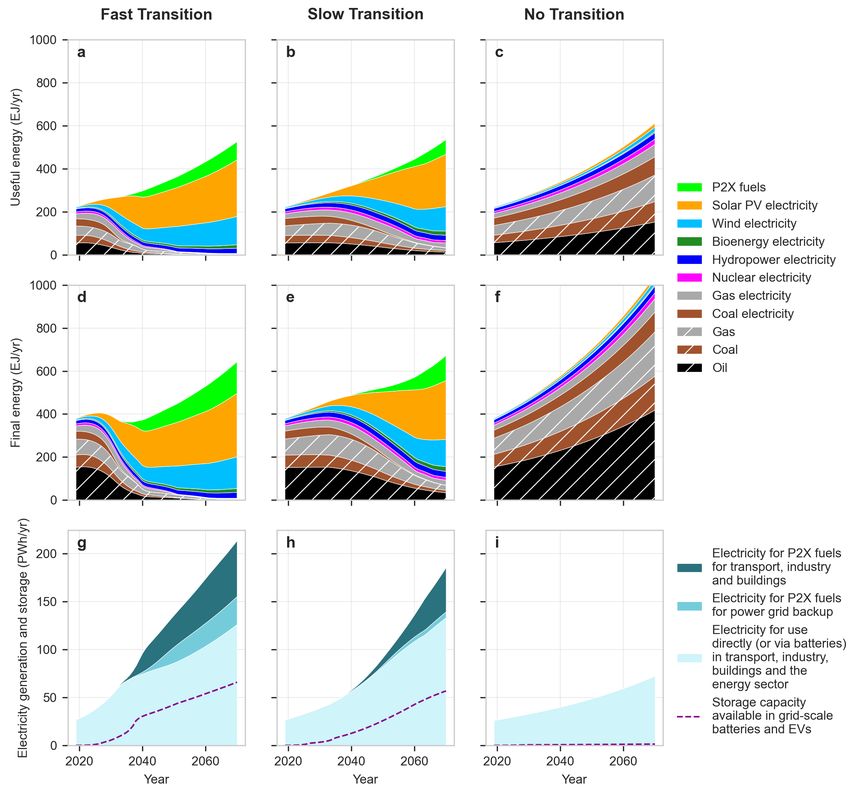
Empirically grounded technology forecasts and the
                    energy transition
Rupert Waya,b , Matthew C. Ivesa,b , Penny Mealya,b,c and J. Doyne Farmera,d,e
a
Institute for New Economic Thinking at the Oxford Martin School, University of
                               Oxford, Oxford, UK
b
  Smith School of Enterprise and the Environment, University of Oxford, Oxford,
                                        UK
      c
        SoDa Labs, Monash Business School, Monash University, Australia
           d
             Mathematical Institute, University of Oxford, Oxford, UK
                e
                  Santa Fe Institute, Santa Fe, New Mexico, USA

                                   September 14, 2021

Rapidly decarbonising the global energy system is critical for addressing climate change,
but concerns about costs have been a barrier to implementation. Most energy-economy
models have historically underestimated deployment rates for renewable energy tech-
nologies and overestimated their costs 1,2,3,4,5,6 . The problems with these models have
stimulated calls for better approaches 7,8,9,10,11,12 and recent e↵orts have made progress in
this direction 13,14,15,16 . Here we take a new approach based on probabilistic cost fore-
casting methods that made reliable predictions when they were empirically tested on
more than 50 technologies 17,18 . We use these methods to estimate future energy system
costs and find that, compared to continuing with a fossil-fuel-based system, a rapid green
energy transition will likely result in overall net savings of many trillions of dollars -
even without accounting for climate damages or co-benefits of climate policy. We show
that if solar photovoltaics, wind, batteries and hydrogen electrolyzers continue to follow
their current exponentially increasing deployment trends for another decade, we achieve
a near-net-zero emissions energy system within twenty-five years. In contrast, a slower
transition (which involves deployment growth trends that are lower than current rates)
is more expensive and a nuclear driven transition is far more expensive. If non-energy
sources of carbon emissions such as agriculture are brought under control, our analysis
indicates that a rapid green energy transition would likely generate considerable eco-
nomic savings while also meeting the 1.5 degrees Paris Agreement target.
Future energy system costs will be determined by a combination of technologies that pro-
duce, store and distribute energy. Their costs and deployment will change with time due to
innovation, economic competition, public policy, concerns about climate change and other
factors. Figure 1 provides an historical perspective for how the energy landscape has evolved
over the last 140 years. Panel (a) shows the historical costs of the principal energy technolo-
gies and panel (b) gives their deployment, both on a logarithmic scale. As we approach the
present in panel (a), the diagram becomes more congested, making it clear that we are in a
period of unprecedented energy diversity, with many technologies with global average costs
around $100/MWh competing for dominance.

                                              1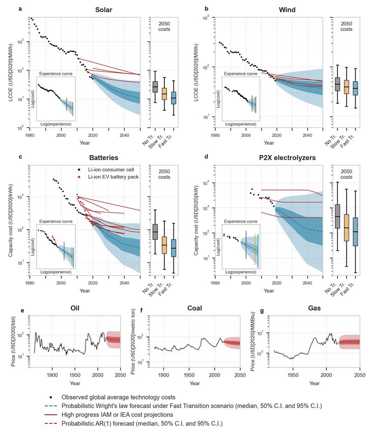
The long term trends provide a clue as to how this competition may be resolved: The
prices of fossil fuels such as coal, oil and gas are volatile, but after adjusting for inflation,
prices now are very similar to what they were 140 years ago, and there is no obvious long
range trend. In contrast, for several decades the costs of solar photovoltaics (PV), wind, and
batteries have dropped (roughly) exponentially at a rate near 10% per year. The cost of solar
PV has decreased by more than three orders of magnitude since its first commercial use in
1958.

Figure 1: Historical costs and production of key energy supply technologies. (a) Inflation-adjusted
useful energy costs (or in some cases prices) as a function of time. We show useful energy because
it takes conversion efficiency into account (see Supplementary Note (SN) 1.7). Electricity generation
technology costs are levelized costs of electricity (LCOEs). Battery series show capital cost per cycle
and energy stored per year, assuming daily cycling for 10 years (these are not directly comparable
with other data series here). Modelled costs of power-to-X (P2X) fuels, such as hydrogen or ammonia,
assume historical electrolyzer costs and a 50-50 mix of solar and wind electricity. (b) Global useful
energy consumption. The provision of energy from solar photovoltaics has, on average, increased at
44% per year for the last 30 years, while wind has increased at 23% per year. These are just a few
representative time series, for a full description of data and methods see SN6.

    Figure 1(b) shows how the use of technologies in the global energy landscape has evolved
since 1880. It documents the slow exponential rise in the production of oil and natural gas
over a century, until they eventually replaced traditional biomass and equalled coal, as well
as the rapid rise and plateauing of nuclear energy. But perhaps the most remarkable feature is
the dramatic exponential rise in the deployment of solar PV, wind, batteries and electrolyzers
over the last decades as they transitioned from niche applications to mass markets. Their
rate of increase is similar to that of nuclear energy in the 70’s, but unlike nuclear energy,
they have all consistently experienced exponentially decreasing costs. The combination of
exponentially decreasing costs and rapid exponentially increasing deployment is di↵erent to
anything observed in any other energy technologies in the past, and positions renewables to
challenge the dominance of fossil fuels within a decade.
    Will clean energy technology costs continue to drop at the same rates in the future? What
does this imply for the overall cost of the green energy transition? Is there a path forward

                                                  2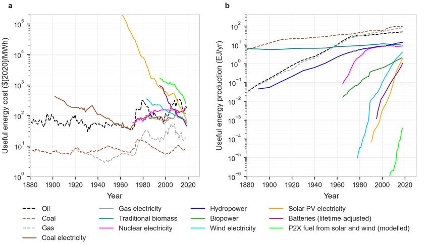
that can get us there cheaply and quickly? We address these questions here.
How good were past energy forecasts?
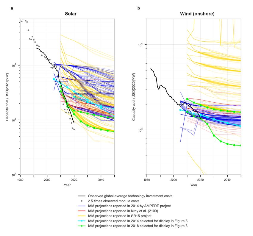
Sound energy investments require reliable forecasts. As illustrated in Figure 2(a), past pro-
jections of present renewable energy costs by influential energy-economy models have con-
sistently been much too high. (“Projections” are forecasts conditional on scenarios, so we
use the terms interchangeably.) The inset of the figure gives a histogram of 2,905 projections
by integrated assessment models, which are perhaps the most widely used type of global
energy-economy models 19,20,21,22 , for the annual rate at which solar PV system investment
costs would fall between 2010 and 2020 19 . The mean value of these projected cost reduc-
tions was 2.6%, and all were less than 6%. In stark contrast, during this period solar PV costs
actually fell by 15% per year. Such models have consistently failed to produce results in line
with past trends 3,23 . Considering their central role in guiding energy investment decisions
and climate policy, the consequences of such systematic bias in modelling projections are
alarming. Failing to appreciate cost improvement trajectories of renewables relative to fossil
fuels not only leads to under-investment in critical emission reduction technologies, it also
locks in higher cost energy infrastructure for decades to come. In contrast, forecasts based
on trend extrapolation consistently performed much better 24,25,26,27 .
Some reasons for the poor performance of energy-economy models include their seem-
ingly arbitrary assumptions regarding the maximum deployment and maximum growth rates
of renewables, plus the imposition of “floor costs”, i.e. fixed levels that costs are assumed
never to fall below 28 . As shown in Figure 2(b), past floor costs used in IAMs have repeatedly
been violated. We know of no good empirical evidence supporting floor costs and do not
impose them. (For a critique of other aspects of standard energy-economy models, see 29,8,9 ).
3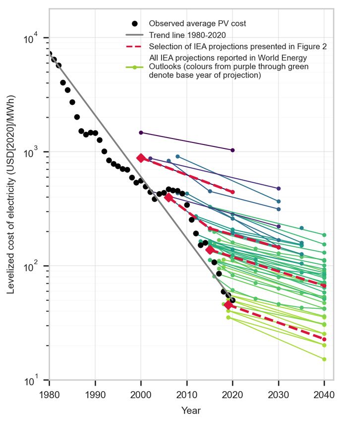
Figure 2: Historical PV cost forecasts and floor costs. (a) The black dots show the observed global
average levelized cost of electricity (LCOE) over time. Red lines are LCOE projections reported by
the International Energy Agency (IEA), dark blue lines are integrated assessment model (IAM) LCOE
projections reported in 2014 19 and light blue lines are IAM projections reported in 2018 20,21 . IAM
projections are rooted in 2010 despite being produced in later years. The projections shown are ex-
clusively “high technological progress” cost trajectories drawn from the most aggressive mitigation
scenarios, corresponding to the biggest projected cost reductions used in these models. Other pro-
jections made were even more pessimistic about future PV costs. The inset compares a histogram of
projected compound annual reduction rates of PV system investment costs from 2010 to 2020 to what
actually occurred (based on all 2,905 scenarios for which the data is available 19 ). (b) PV system floor
costs implemented in a wide range of IAMs. The colours denote the year the floor cost was reported,
ranging from 1997 (dark green) to 2020 (light green). Observed PV system costs are also shown. The
cost of PV modules scaled by a constant factor of 2.5 is provided as a reference. For further details
and data sources see Extended Data Figures 6 and 7(a), and SN6.10

Predicting future technology costs
The diversity of historical cost improvement rates seen in Figure 1(a) applies to technologies
in general 30,25,17,18 . For the vast majority of technologies, inflation-adjusted costs remain
roughly constant through time. In contrast, for some technologies, such as optical fibers,
solar PV or transistors, costs drop roughly exponentially, at rates ranging from over 50% per
year to a few percent per year 31 (SN8.1). Once a track record is established, the rates of
improvement tend to remain constant. While there are occasionally breaks in the trend, this
is rare.
    In contrast to the energy-economy models mentioned above, during the past decade sim-
ple time series models have been shown to make reliable forecasts of technology costs 32,25,33,18 .
In this study we apply these methods to key energy technologies and use them to make prob-
abilistic estimates for the cost of providing energy services under several di↵erent scenarios.
    For renewable technologies we use a stochastic generalization of Wright’s law, which pre-
dicts that costs drop as a power law of cumulative production. This relationship is also called

                                                   4
an experience curve or learning curve, and cumulative production is also called experience. Ex-
perience does not directly cause costs to drop, but is believed to be correlated with other
factors that do, such as level of e↵ort and R&D, and has the essential advantage of being
relatively easy to measure 34,35 . Forecasting using this model requires estimating two param-
eters for each technology, corresponding to a progress rate and a volatility (see Methods).
In addition, there is an autocorrelation parameter that is common to all technologies. For a
discussion of challenges and caveats concerning Wright’s law see SN8.2.
Successful technologies tend to follow an “S-curve” for deployment, starting with a long
phase of exponential growth in production that eventually tapers o↵ due to market satura-
tion 36 . Under Wright’s law, during the exponential growth phase, costs drop exponentially
in time according to a generalized form of Moore’s law, which is consistent with the historical
behavior of renewable energy technologies. When growth eventually slows, under Wright’s
law, improvement slows down. (For a discussion of causality see SN8.2.1.)
Wright’s law is already widely used in energy system models 37,38,39 , though to the best of
our knowledge, only deterministic implementations have been used so far. Our key contri-
bution here takes advantage of new results that extend Wright’s law to provide an estimate
of the probability distribution of future technology costs, thus providing an estimate of fore-
casting uncertainty. This method was carefully tested by making forecasts at reference dates
in the past, using only the data available at the time, and making predictions over all time
horizons up to 20 years into the future with respect to each reference date. This was done
using historical data for 50 di↵erent technologies, for a total of roughly 6,000 forecasts. The
forecasting accuracy closely matched a priori derived estimates on all time horizons 17,18 .
Because fossil fuel costs have not changed in the long run, they require a di↵erent time
series forecasting model. Since costs have not dropped with experience 40 , the stochastic form
of Wright’s law that we use here reduces to a geometric random walk without drift. This is a
common model for financial time series, including tradeable commodities such as oil or gas,
and can be justified based on the efficient markets hypothesis. On short timescales (say ten
years or less) this is a reasonable approximation, but over longer timescales it predicts too
much volatility in comparison to the historical record. Fossil fuel prices show mean reversion
on longer timescales and are better captured by an AR(1) autoregressive process 41 .
We thus use a univariate AR(1) model to forecast coal, oil, and gas (see Methods), SN5.1
and SN6.1-6.3). While coal-fired electricity and gas-fired electricity showed significant drops
in cost for some of the twentieth century, in the long run their costs are increasingly dom-
inated by fuel costs 42 , so we use the AR(1) model for these as well (SN6.4-6.5). The tech-
nologies for which we use Wright’s law to generate probabilistic cost forecasts are: solar PV,
wind, batteries, electrolyzers, nuclear power, biopower and hydropower. While the first four
of these technologies have strong historical progress trends, the latter three have either flat
or rising costs, so have less potential to play a significant role in energy transition, and hence
are less important in this analysis (SN6.6-6.12).
Figure 3 shows probabilistic forecasts for seven key energy technologies under a rapid
energy transition scenario that we will define in a moment. Each renewable technology ini-
tially follows its current trend of exponential decreasing costs, which slows when it becomes
dominant and its rate of deployment drops. We also show a selection of cost projections
reported by IAM and IEA studies. We show only their most optimistic projections, i.e. low
cost projections that correspond to high technological progress scenarios. Consistent with
the historical behavior of these models illustrated in Figure 2, these projections are high rel-
ative to historical trends. Although viewed as highly optimistic, they are all higher than our
median forecasts, and except for wind, substantially higher.
5Figure 3: Technology forecasts. (a - d) The main plots show cost forecast distributions under our Fast
Transition scenario for solar PV, wind, batteries and polymer electrolyte membrane (PEM) electrolyz-
ers; the 50% confidence interval is dark blue and the 95% confidence interval is light blue. These are
compared to several representative current and past projections corresponding to “optimistic” miti-
gation scenarios made by IAMs and the IEA (red lines). (See Extended Data Figure 7.) For batteries we
show both consumer cells and electric vehicle (EV) battery pack prices, though these are now almost
identical; our forecasts are based on consumer cells while the IEA forecasts shown are based on EV
batteries. The box and whisker plots in the right-hand panels compare cost forecasts in 2050 under
our three di↵erent scenarios (defined shortly). The insets show historical experience curves and fore-
casts, with progress rates that are independent of the scenario, and vertical lines indicating how far
each technology moves down the probabilistic experience curve in each scenario. Panels (e - g) give
probabilistic cost forecasts for oil, coal and gas based on the AR(1) time series model. (See SN6 for
details of data sources and model calibration.)
6The stochastic version of Wright’s law we use here captures the historical volatility of
past performance and the resulting estimation error, and projects this uncertainty forward
in future cost distributions. It thus provides cost ranges that are supported by empirical
evidence, as opposed to the ad hoc ranges that are often used 43 . The insets show costs vs.
experience and emphasize that median costs develop identically as a function of experience in
all scenarios. The side panels of Figure 3 illustrate that under Wright’s law forecasts depend
on the scenario; as a result, under a rapid transition, we reach lower costs sooner.
From single technologies to a full system model
Technology cost forecasts are conditional on scenarios, which specify energy technology de-
ployment trajectories as a function of time. Our approach to scenario construction di↵ers
from that currently used in standard energy-economy models. In integrated assessment mod-
els, scenarios are the result of optimizing discounted consumption (as measured by GDP)
under constraints on carbon emissions 44 . In simulation models such as the IEA’s World En-
ergy Model, scenarios are the result of choosing the cheapest available technologies through
time, subject to policy choices. Both of these methods require many cost forecasts to be made,
either exogenously or endogenously, during the scenario construction process, via some com-
bination of models and expert forecasts. (Expert forecasts have a poor track record 45 .) Thus
scenarios depend on cost forecasts and vice versa, and small forecasting errors can quickly
get amplified, leading to scenarios that are inconsistent with empirically observed trends.
We instead follow earlier energy system models 46 and construct scenarios exogenously
by specifying how much energy or storage will be provided by each technology as a func-
tion of time (SN2.1). We classify energy services into four categories – transport, industry,
buildings and energy sector self-use (SN1.3) – and assume that end-use sector demand grows
at the historically observed overall rate of 2% per year. We impose the constraint that all
scenarios must reliably provide identical levels of energy services throughout the economy.
This method has the advantage of being simple and transparent, and allows us to follow
long-standing deployment trends, which are at least known to have been feasible from the
past until the present. This is in contrast to the optimal scenarios generated by IAMs, which
typically do not even attempt to match historical behavior 47 .
The three scenarios that we consider are shown in Figure 4. They run from 2019 to 2070,
and were chosen to represent three distinctly di↵erent energy system pathways. In the Fast
Transition scenario (panels a, d, g), renewable energy and storage technologies maintain their
current deployment growth rates for a decade, replacing fossil fuels in two decades. Follow-
ing a standard S-curve, once renewables become dominant, deployment slows to grow at
2% per year. Short term storage and electrification of most transport are achieved with bat-
teries, while long term energy storage and all hard-to-electrify applications are served by
power-to-X fuels, i.e. by using electricity for hydrogen electrolysis and either directly using
hydrogen or using it to make other fuels such as ammonia and methane as needed 48 . This
corresponds to an “electrify almost everything” scenario, with full sector-coupling 49 . In the
Slow Transition scenario (panels b, e, h), in contrast, current rapid deployment trends for
renewables slow down immediately, so that fossil fuels are phased out more slowly and con-
tinue to dominate until mid-century. Finally, in the No Transition scenario (panels, c, f, i), the
energy system remains similar to its current form and each source of energy grows propor-
tionally, making this close to typical “worst case” scenarios (which were until recently called
“business as usual” scenarios). (Scenario details are shown in SN4.)
7Figure 4: Scenarios. The three columns represent each of the scenarios. The rows are: (1) Annual
useful energy provided by each technology as a function of time. (2) Annual final energy provided
by each technology as a function of time. (3) Annual electricity generation and storage in grid-scale
batteries and EV batteries; total generation is divided between final electricity delivered to the econ-
omy and electricity used to produce P2X fuels for hard-to-electrify applications and for power grid
backup.
Our approach is based on two key design principles: 1) include only the minimal set of
variables necessary to represent most of the global energy system, and the most important
cost and production dynamics, and 2) ensure all assumptions and dynamics are technically
realistic and closely tied to empirical evidence (SN1.1). This means that we focus on en-
ergy technologies that have been in commercial use for sufficient time to develop a reliable
historical record.
We choose a level of model granularity well suited to the probabilistic forecasting meth-
ods used, i.e. one that allows accurate model calibration, and ensures overall cost-reduction
trends associated with cumulative production are captured for each technology. Our model
design can be run on a laptop, is easy to understand and interpret, and allows us to calibrate
all components against historical data so that the model is firmly empirically grounded. The
historical data does not exist to do this on a more granular level.
8Consistent with our two design principles, we have deliberately omitted several minor
energy technologies. Co-generation of heat, traditional biomass, marine energy, solar ther-
mal energy, and geothermal energy were omitted either due to insufficient historical data or
because they have not exhibited significant historical cost improvements, or both. Liquid
biofuels were also excluded because any significant expansion would have high environmen-
tal costs (SN1.5.4). Finally, carbon capture and storage (CCS) in conjunction with fossil fuels
was omitted because i) it is currently a very small, low growth sector, ii) it has exhibited no
promising cost improvements so far in its 50 year history, and iii) the cost of fossil fuels pro-
vides a hard lower bound on the cost of providing energy via fossil fuels with CCS (SN1.6.1).
This means that within a few decades electricity produced with CCS will likely not be com-
petitive even if CCS is free. The major technologies that we do include cover 90% of current
final energy, excluding energy carriers that are already renewable such as bioenergy and bio-
fuels, plus petrochemical feedstock, which is not an energy carrier. See SN1 for a complete
description of the model.
Since renewables are intermittent, storage is essential. In the Fast Transition scenario
we have allocated so much storage capacity using batteries and P2X fuels that the entire
global energy system could be run for a month without any sun or wind (SN3). This is a
sensible choice because both batteries and electrolyzers have highly favorable trends for cost
and production (SN6.11-6.12). From 1995 to 2018 the production of lithium ion batteries
increased at 30% per year, while costs dropped at 12% per year, giving an experience curve
comparable to that of solar PV 50 . Currently, about 60% of the cost of electrolytic hydrogen
is electricity, and hydrogen is around 80% of the cost of ammonia 51 , so these automatically
take advantage of the high progress rates for solar PV and wind.
To understand these scenarios it is important to distinguish final energy, which is the en-
ergy delivered for use in sectors of the economy, from useful energy, which is the portion of
final energy used to perform energy services, such as heat, light and kinetic energy (SN1.2).
Fossil fuels tend to have large conversion losses in comparison to electricity, which means
that significantly more final energy needs to be produced to obtain a given amount of use-
ful energy. Switching to energy carriers with higher conversion efficiencies (e.g. moving to
electric vehicles) significantly reduces final energy consumption 52,11 . Our Fast Transition
scenario assumes that eventually almost all energy services originate with electricity gen-
erated by solar PV and wind, making and burning P2X fuels or using batteries when it is
impractical to use renewables directly. As shown by comparing Figures 4(g) and 4(i), the Fast
Transition substantially increases the role of electricity in the energy system.
How much will each scenario cost?
There are many di↵erent approaches to modelling energy system pathway costs 53,54 . We use
the “direct engineering costs” approach, in which the overall cost of a scenario is computed
by adding up the costs of the component technologies (SN1.8). We sum the costs of direct-use
oil, coal and gas; electricity generated by seven di↵erent technologies; plus utility-scale grid
batteries and electrolyzers; and additional infrastructure for expansion of the electricity grid
(SN3.7). For electricity generation costs we use the LCOE metric. This is particularly advan-
tageous here because then the experience curve formulation inherently captures historical
progress trends in all LCOE components, including capital costs, capacity factors, and inter-
est rates, which would otherwise be hard to forecast separately. We estimate infrastructure
costs that are not directly covered by technologies included in the model, e.g. for fuel storage
and distribution (SN1.6.4) or for fueling or charging light duty vehicles (SN1.6.5), and argue
that they are roughly the same across scenarios.
To apply our probabilistic technology cost forecasting methods in a given scenario, we
9employ a Monte Carlo approach, simulating many di↵erent future cost trajectories, then
exponentially discounting future costs to calculate the expected net present cost of the sce-
nario, up to 2070 (SN5.5, SN7.1). Figure 5(a) shows median total costs through time for each
scenario, showing how the Fast Transition rapidly transfers energy expenditures from fossil
fuels to renewables. Figure 5(b) shows that, although there is considerable uncertainty, the
net present cost is likely to be substantially lower. Figure 5(d) shows how the Fast Transition
rapidly decreases energy system emissions, making it feasible to achieve the Paris Agreement
if non-energy related sources of emissions are also brought under control (SN8.6.1). In con-
trast, the Slow Transition is not as cheap as the Fast Transition. This is because the current
high spending on fossil fuels continues for decades and the savings from renewables are only
realized much later. Nonetheless, it also generates savings relative to No Transition.
Previous analyses have suggested that whether or not it makes good economic sense to
quickly transition to clean energy technologies depends on the discount rate 22,55 . In Fig-
ure 5(c) we show a striking result: the Fast Transition is likely to be substantially cheaper at
all reasonable discount rates. Using the 1.4% social discount rate recommended in the Stern
Review 56 , for example, the expected net present saving is roughly $14 trillion. The me-
dian value, which gives a better indication of the net present saving likely to be realized in
practice, is roughly $26 trillion. (The distribution of costs is roughly log-normal, so means
and medians are substantially di↵erent.) Note that there is some evidence that technological
progress does not slow when technologies reach their saturation phase 57 . If this is true, then
costs continue to drop at their current pace according to Moore’s law, and the Fast Transition
saves substantially more relative to the other scenarios (see SN7.4).
10Figure 5: Scenario costs and emissions. (a) Median annual expenditures on fossil fuel and non fossil
fuel technologies in each scenario in trillions of dollars (tn USD). (b) Forecast distributions of the net
present cost (NPC) of each scenario, for a fixed discount rate of 2%. (c) Expected net present cost
of each scenario relative to the No Transition scenario as a function of the discount rate. (d) Carbon
emissions as a function of time.
We constructed an additional scenario in which nuclear plays a dominant role in replacing
fossil fuels (SN4.4), but this is substantially more expensive than the baseline. For example,
using a 1.4% discount rate the mean cost is about 15 trillion dollars more than No Transition
and 27 trillion more than the Fast Transition (SN7.1).
To enhance the credibility of our estimates we have used consistently conservative as-
sumptions regarding the costs, performance and operational requirements of clean energy
technologies, and done the opposite for fossil fuels. Our systematic use of technologies with
appropriate price histories means that in many cases we were forced to neglect solutions that
are promising avenues of cost reduction, such as demand-side management of power grids
and end-use efficiency improvements 11 . As a result, it is likely that the future costs of the
renewable transition will be substantially lower than the estimates presented here (SN1.8).
Our analysis is based on global averages, but there is a wide geographic variation in en-
ergy costs. Within countries, renewables tend to be deployed first in regions where their costs
are favorable, but that is not the case globally (SN8.4). In any case, under the Fast Transition
regional cost di↵erences are quickly overcome through time. For solar PV, for example, his-
torically the 95th percentile of geographical cost variation at a given point in time became
equivalent to the 5th percentile in less than a decade (SN8.4). Because costs are summed,
global averages are sufficient to estimate costs, and we expect that future e↵orts will take
11advantage of geographic variation to achieve even cheaper solutions.
Although the Fast Transition happens quickly it is still possible to replace the energy sys-
tem without excessive stranding of capital. Lifetimes of large energy infrastructure projects
typically range from 25 to 50 years, meaning that on average about 2-4% of capacity needs
replacing in any given year. In addition, useful energy demand grows at 2% per year. These
two factors make it possible for renewables to replace most of the existing energy system in
20 years and replace the remaining 5% within a few decades without necessarily stranding
assets beyond their economic lifetime.
Discussion
As we have not systematically searched the space of all possible scenarios, we do not claim
that the Fast Transition scenario presented here is the cheapest possibility. Given the rela-
tively low cost of gas, it could be possible to achieve cheaper scenarios by using gas in place
of P2X fuels in some applications, but these of course would not be zero-emissions systems.
Similarly, while fossil fuel costs have not historically trended down, competition from renew-
ables may force them down, though this is feasible only at substantially reduced production
levels where the cheapest fossil fuel producers are competitive 58 . This suggests that, while
most of the Fast Transition is aligned with market forces, policies that discourage the use of
fossil fuels will likely still be needed to fully decarbonize energy.
In response to our opening question, "Is there a path forward that can get us there cheaply
and quickly?", our answer is an emphatic "Yes!". Our quantitative analysis supports other
recent e↵orts using up-to-date data and technology assumptions that reach a similar conclu-
sion 59,60,13,14,15,16 . The key is to maintain the current high growth rates of rapidly progress-
ing clean energy technologies for the next decade. This is required to build up the industrial
capabilities and technical know-how necessary to produce, install and operate these tech-
nologies at scale as fast as possible so that we can profit from the resulting cost reductions
sooner rather than later.
The belief that the green energy transition will be expensive has been a major driver of the
ine↵ective response to climate change for the last forty years. This pessimism is at odds with
past technological cost-improvement trends, and risks locking humanity into an expensive
and dangerous energy future. While arguments for a rapid green transition often cite benefits
such as the avoidance of climate damages, less air pollution and lower energy price volatility
(SN8.6), these benefits are often contrasted against discussions about the associated costs of
transitioning 44 . Our analysis suggests that such trade-o↵s are unlikely to exist: a greener,
healthier and safer global energy system is also likely to be cheaper. Updating expectations to
better align with historical evidence could fundamentally change the debate about climate
policy and dramatically accelerate progress to decarbonise energy systems around the world.
Methods
Time-series models
We employ two time-series models for forecasting technology costs. The first is a first-
di↵erence stochastic form of Wright’s law, developed and tested by Lafond et al. 18 , which
models costs dropping as a power law of cumulative production. Let ct be the cost and zt be
the experience of a given technology at time t, and let ut ⇠ N (0, u2 ) be an IID draw from a
normal distribution. Then future costs are predicted using the iterative relationship
log ct log ct 1 = ! (log zt log zt 1 ) + ut + ⇢ut 1 . (1)
12This relationship has three parameters. For a given technology, the experience exponent
! characterizes the average rate at which costs drop as a function of experience, and the noise
variance u2 characterizes the variability of this relationship. The autocorrelation parameter
⇢ characterizes the persistence of fluctuations in cost improvements. To avoid overfitting we
use ⇢ = 0.19 for all technologies, which was found by Lafond et al. 18 to be a good overall
choice for 50 di↵erent technologies. (We also did a comparison of all our results replacing
Wright’s Law by a generalized form of Moore’s Law (see SN7.4)).
When applying the model to technologies with falling costs, as shown in Figure 3, two
features of the model must be stressed. First, the Wright’s law model does not simply “as-
sume” that if costs fell in the past then they will fall in future – indeed, costs are predicted to
rise with a non-zero probability that depends directly on observed data in the past. Second,
despite the downward trends, all cost forecast distributions are always strictly positive, since
costs develop in log space.
For fossil fuels we use an AR(1) process of the form
2
log ct = log ct 1+ (µ log ct 1 ) + ✏t , with IID ✏t ⇠ N (0, ✏ ), (2)
where µ = E[log ct ] is the unconditional mean of the logarithm of cost, ✏ is the volatility of
the noise process and is the rate of mean reversion. For more details on forecasting methods
see SN5.
Scenario construction
We construct energy transition scenarios by assuming that growth rates follow logistic (or
“S”) curves with a specified start and end point consistent with the growth of total useful
energy. We model the conversion process based on average final-to-useful energy conversion
efficiency factors given by DeStercke 61 . The endpoint of each scenario in 2070 is defined by
the shares of technologies providing electricity generation and the shares of energy carriers
providing final energy. The start points for all scenarios are identical and match the current
shares in 2018. Details of all growth rates, timings and energy carrier mixes for each scenario
are given in SN2 and SN4.
Data availability
We use data from many sources, mostly free and openly available on the internet, but occa-
sionally via standard university-wide subscription licenses held by the University of Oxford.
Production data comes mostly from the International Energy Agency 62 and BP’s Statis-
tical Review of World Energy 63 . Cost data is much harder to find and comes from a wide
variety of sources including, among others, Lazard’s Levelized Cost of Energy Analyses 64 ,
the International Renewable Energy Agency 65 , the U.S. Energy Information Administration’s
Annual Energy Outlooks 66 , Bloomberg New Energy Finance (BNEF) and Bloomberg L.P. (via
Bloomberg Terminal). For more details on data sources see SN6.
Code availability
The code and data used in this analysis will be made available upon request.
References
[1] Felix Creutzig, Peter Agoston, Jan Christoph Goldschmidt, Gunnar Luderer, Gregory
Nemet, and Robert C. Pietzcker. The underestimated potential of solar energy to mit-
13igate climate change. Nature Energy, 2(9):17140, Aug 2017. ISSN 2058-7546. doi:
10.1038/nenergy.2017.140. URL https://doi.org/10.1038/nenergy.2017.140.
[2] Mengzhu Xiao, Tobias Junne, Jannik Haas, and Martin Klein. Plummeting costs of re-
newables - are energy scenarios lagging? Energy Strategy Reviews, 35:100636, 2021.
ISSN 2211-467X. doi: https://doi.org/10.1016/j.esr.2021.100636. URL https://www.
sciencedirect.com/science/article/pii/S2211467X21000225.
[3] Marc Jaxa-Rozen and Evelina Trutnevyte. Sources of uncertainty in long-term global
scenarios of solar photovoltaic technology. Nature Climate Change, 11(3):266–273, Mar
2021. ISSN 1758-6798. doi: 10.1038/s41558-021-00998-8. URL https://doi.org/10.
1038/s41558-021-00998-8.
[4] Auke Hoekstra, Maarten Steinbuch, and Geert Verbong. Creating agent-based energy
transition management models that can uncover profitable pathways to climate change
mitigation. Complexity, 2017:1967645, Dec 2017. ISSN 1076-2787. doi: 10.1155/2017/
1967645. URL https://doi.org/10.1155/2017/1967645.
[5] Hiroto Shiraki and Masahiro Sugiyama. Back to the basic: toward improvement of
technoeconomic representation in integrated assessment models. Climatic Change, 162
(1):13–24, Sep 2020. ISSN 1573-1480. doi: 10.1007/s10584-020-02731-4. URL https:
//doi.org/10.1007/s10584-020-02731-4.
[6] Marta Victoria, Nancy Haegel, Ian Marius Peters, Ron Sinton, Arnulf Jäger-Waldau,
Carlos del Cañizo, Christian Breyer, Matthew Stocks, Andrew Blakers, Izumi Kaizuka,
Keiichi Komoto, and Arno Smets. Solar photovoltaics is ready to power a sustainable
future. Joule, 5(5):1041–1056, 2021. ISSN 2542-4351. doi: https://doi.org/10.1016/
j.joule.2021.03.005. URL https://www.sciencedirect.com/science/article/pii/
S2542435121001008.
[7] Nicholas Stern. Economics: Current climate models are grossly misleading. Nature,
530(7591):407–409, Feb 2016. ISSN 1476-4687. doi: 10.1038/530407a. URL https:
//doi.org/10.1038/530407a.
[8] Robert S. Pindyck. Climate change policy: What do the models tell us? Journal of
Economic Literature, 51(3):860–72, September 2013. doi: 10.1257/jel.51.3.860. URL
https://www.aeaweb.org/articles?id=10.1257/jel.51.3.860.
[9] J Doyne Farmer, Cameron Hepburn, Penny Mealy, and Alexander Teytelboym. A third
wave in the economics of climate change. Environmental and Resource Economics, 62(2):
329–357, 2015.
[10] David L. McCollum, Ajay Gambhir, Joeri Rogelj, and Charlie Wilson. Energy modellers
should explore extremes more systematically in scenarios. Nature Energy, 5(2):104–107,
Feb 2020. ISSN 2058-7546. doi: 10.1038/s41560-020-0555-3. URL https://doi.org/
10.1038/s41560-020-0555-3.
[11] Amory B Lovins, Diana Ürge-Vorsatz, Luis Mundaca, Daniel M Kammen, and Jacob W
Glassman. Recalibrating climate prospects. Environmental Research Letters, 14(12):
120201, 2019.
[12] S. Pye, O. Broad, C. Bataille, P. Brockway, H. E. Daly, R. Freeman, A. Gambhir, O. Geden,
F. Rogan, S. Sanghvi, J. Tomei, I. Vorushylo, and J. Watson. Modelling net-zero emissions
energy systems requires a change in approach. Climate Policy, 21(2):222–231, 2021. doi:
1410.1080/14693062.2020.1824891. URL https://doi.org/10.1080/14693062.2020.
1824891.
[13] Arnulf Grubler, Charlie Wilson, Nuno Bento, Benigna Boza-Kiss, Volker Krey, David L.
McCollum, Narasimha D. Rao, Keywan Riahi, Joeri Rogelj, Simon De Stercke, Jonathan
Cullen, Stefan Frank, Oliver Fricko, Fei Guo, Matt Gidden, Petr Havlík, Daniel Hupp-
mann, Gregor Kiesewetter, Peter Rafaj, Wolfgang Schoepp, and Hugo Valin. A low
energy demand scenario for meeting the 1.5 °c target and sustainable development
goals without negative emission technologies. Nature Energy, 3(6):515–527, 2018.
ISSN 2058-7546. doi: 10.1038/s41560-018-0172-6. URL https://doi.org/10.1038/
s41560-018-0172-6.
[14] Marta Victoria, Kun Zhu, Tom Brown, Gorm B. Andresen, and Martin Greiner. Early
decarbonisation of the european energy system pays o↵. Nature Communications, 11
(1):6223, Dec 2020. ISSN 2041-1723. doi: 10.1038/s41467-020-20015-4. URL https:
//doi.org/10.1038/s41467-020-20015-4.
[15] Gang He, Jiang Lin, Froylan Sifuentes, Xu Liu, Nikit Abhyankar, and Amol Phadke.
Rapid cost decrease of renewables and storage accelerates the decarbonization of china’s
power system. Nature Communications, 11(1):2486, May 2020. ISSN 2041-1723. doi: 10.
1038/s41467-020-16184-x. URL https://doi.org/10.1038/s41467-020-16184-x.
[16] Dmitrii Bogdanov, Manish Ram, Arman Aghahosseini, Ashish Gulagi, Ay-
obami Solomon Oyewo, Michael Child, Upeksha Caldera, Kristina Sadovskaia, Javier
Farfan, Larissa De Souza Noel Simas Barbosa, Mahdi Fasihi, Siavash Khalili, Thure
Traber, and Christian Breyer. Low-cost renewable electricity as the key driver of
the global energy transition towards sustainability. Energy, 227:120467, 2021. ISSN
0360-5442. doi: https://doi.org/10.1016/j.energy.2021.120467. URL https://www.
sciencedirect.com/science/article/pii/S0360544221007167.
[17] J Doyne Farmer and François Lafond. How predictable is technological progress? Re-
search Policy, 45(3):647–665, 2016.
[18] François Lafond, Aimee Gotway Bailey, Jan David Bakker, Dylan Rebois, Rubina
Zadourian, Patrick McSharry, and J Doyne Farmer. How well do experience curves pre-
dict technological progress? a method for making distributional forecasts. Technological
Forecasting and Social Change, 128:104–117, 2018.
[19] Keywan Riahi, Elmar Kriegler, Nils Johnson, Christoph Bertram, Michel den Elzen, Jiy-
ong Eom, Michiel Schae↵er, Jae Edmonds, Morna Isaac, Volker Krey, Thomas Long-
den, Gunnar Luderer, Aurélie Méjean, David L. McCollum, Silvana Mima, Hal Tur-
ton, Detlef P. van Vuuren, Kenichi Wada, Valentina Bosetti, Pantelis Capros, Patrick
Criqui, Meriem Hamdi-Cherif, Mikiko Kainuma, and Ottmar Edenhofer. Locked into
copenhagen pledges — implications of short-term emission targets for the cost and fea-
sibility of long-term climate goals. Technological Forecasting and Social Change, 90:8–
23, 2015. ISSN 0040-1625. doi: https://doi.org/10.1016/j.techfore.2013.09.016. URL
https://www.sciencedirect.com/science/article/pii/S0040162513002539.
[20] Volker Krey, Fei Guo, Peter Kolp, Wenji Zhou, Roberto Schae↵er, Aayushi Awasthy,
Christoph Bertram, Harmen-Sytze de Boer, Panagiotis Fragkos, Shinichiro Fujimori,
Chenmin He, Gokul Iyer, Kimon Keramidas, Alexandre C. Köberle, Ken Oshiro,
Lara Aleluia Reis, Bianka Shoai-Tehrani, Saritha Vishwanathan, Pantelis Capros, Lau-
rent Drouet, James E. Edmonds, Amit Garg, David E.H.J. Gernaat, Kejun Jiang, Maria
15Kannavou, Alban Kitous, Elmar Kriegler, Gunnar Luderer, Ritu Mathur, Matteo Mura-
tori, Fuminori Sano, and Detlef P. van Vuuren. Looking under the hood: A compari-
son of techno-economic assumptions across national and global integrated assessment
models. Energy, 172:1254 – 1267, 2019. ISSN 0360-5442. doi: https://doi.org/10.1016/
j.energy.2018.12.131. URL http://www.sciencedirect.com/science/article/pii/
S0360544218325039.
[21] Daniel Huppmann, Elmar Kriegler, Volker Krey, Keywan Riahi, Joeri Rogelj, Kather-
ine Calvin, Florian Humpenoeder, Alexander Popp, Steven K. Rose, John Weyant, Nico
Bauer, Christoph Bertram, Valentina Bosetti, Jonathan Doelman, Laurent Drouet, Jo-
hannes Emmerling, Stefan Frank, Shinichiro Fujimori, David Gernaat, Arnulf Grubler,
Celine Guivarch, Martin Haigh, Christian Holz, Gokul Iyer, Etsushi Kato, Kimon
Keramidas, Alban Kitous, Florian Leblanc, Jing-Yu Liu, Konstantin Lö✏er, Gunnar Lud-
erer, Adriana Marcucci, David McCollum, Silvana Mima, Ronald D. Sands, Fuminori
Sano, Jessica Strefler, Junichi Tsutsui, Detlef Van Vuuren, Zoi Vrontisi, Marshall Wise,
and Runsen Zhang. IAMC 1.5°C Scenario Explorer and Data hosted by IIASA. Technical
report, IIASA, August 2019. URL https://doi.org/10.5281/zenodo.3363345.
[22] William D Nordhaus. Revisiting the social cost of carbon. Proceedings of the National
Academy of Sciences, 114(7):1518–1523, 2017.
[23] C. Wilson, A. Grubler, N. Bauer, V. Krey, and K. Riahi. Future capacity growth of energy
technologies: are scenarios consistent with historical evidence? Climatic Change, 118(2):
381–395, May 2013. ISSN 1573-1480. doi: 10.1007/s10584-012-0618-y. URL https:
//doi.org/10.1007/s10584-012-0618-y.
[24] Charles D. Ferguson, Lindsey E. Marburger, J. Doyne Farmer, and Arjun Makhijani.
A US nuclear future? Nature, 467(7314):391–393, sep 2010. ISSN 0028-0836. doi:
10.1038/467391a. URL http://www.nature.com/articles/467391a.
[25] Béla Nagy, J Doyne Farmer, Quan M Bui, and Jessika E Trancik. Statistical basis for
predicting technological progress. PloS one, 8(2):e52669, 2013.
[26] D.E. Carlson. The Status and Outlook for the Photovoltaics Industry. Technical report,
BP, 2006. URL https://www.aps.org/meetings/multimedia/upload/The_Status_
and_Outlook_for_the_Photovoltaics_Industry_David_E_Carlson.pdf.
[27] Noah Kittner, Felix Lill, and Daniel M. Kammen. Energy storage deployment and inno-
vation for the clean energy transition. Nature Energy, 2(9):17125, Jul 2017. ISSN 2058-
7546. doi: 10.1038/nenergy.2017.125. URL https://doi.org/10.1038/nenergy.
2017.125.
[28] E De Cian, J Buhl, S Carrara, M Bevione, S Monetti, and H Berg. Learning in inte-
grated assessment models and initiative based learning-an interdisciplinary approach.
PATHWAYS Deliverable, 3, 2016.
[29] Ajay Gambhir, Isabela Butnar, Pei-Hao Li, Pete Smith, and Neil Strachan. A re-
view of criticisms of integrated assessment models and proposed approaches to ad-
dress these, through the lens of beccs. Energies, 12(9), 2019. ISSN 1996-1073. doi:
10.3390/en12091747. URL https://www.mdpi.com/1996-1073/12/9/1747.
[30] Heebyung Koh and Christopher L. Magee. A functional approach for studying tech-
nological progress: Extension to energy technology. Technological Forecasting and So-
cial Change, 75(6):735–758, 2008. ISSN 0040-1625. doi: https://doi.org/10.1016/j.
16techfore.2007.05.007. URL https://www.sciencedirect.com/science/article/pii/
S0040162507001230.
[31] Heebyung Koh and Christopher L Magee. A functional approach for studying techno-
logical progress: Application to information technology. Technological Forecasting and
Social Change, 73(9):1061–1083, 2006.
[32] Stephan Alberth. Forecasting technology costs via the experience curve—myth or
magic? Technological Forecasting and Social Change, 75(7):952–983, 2008.
[33] Jessika E Trancik, Joel Jean, Goksin Kavlak, Magdalena M Klemun, Morgan R Edwards,
James McNerney, Marco Miotti, Patrick R Brown, Joshua M Mueller, and Zachary A
Needell. Technology improvement and emissions reductions as mutually reinforcing
e↵orts: Observations from the global development of solar and wind energy. Technical
report, MIT, 2015.
[34] William D. Nordhaus. The perils of the learning model for modeling endogenous tech-
nological change. The Energy Journal, Volume 35(1), Jan 2014. ISSN 1944-9089. doi:
10.5547/01956574.35.1.1. URL http://www.iaee.org/en/publications/ejarticle.
aspx?id=2546.
[35] Jan Witajewski-Baltvilks, Elena Verdolini, and Massimo Tavoni. Bending the learning
curve. Energy Economics, 52:S86–S99, 2015. ISSN 0140-9883. doi: https://doi.org/10.
1016/j.eneco.2015.09.007. URL https://www.sciencedirect.com/science/article/
pii/S0140988315002601. Frontiers in the Economics of Energy Efficiency.
[36] Arnulf Grübler, Nebojša Naki’enovi’, and David G. Victor. Dynamics of energy tech-
nologies and global change. Energy Policy, 27(5):247–280, may 1999. ISSN 03014215.
doi: 10.1016/S0301-4215(98)00067-6.
[37] Gabrial Anandarajah, Will McDowall, and Paul Ekins. Decarbonising road transport
with hydrogen and electricity: Long term global technology learning scenarios. Interna-
tional Journal of Hydrogen Energy, 38(8):3419–3432, 2013.
[38] Clara F Heuberger, Edward S Rubin, Iain Sta↵ell, Nilay Shah, and Niall Mac Dowell.
Power capacity expansion planning considering endogenous technology cost learning.
Applied Energy, 204:831–845, 2017.
[39] Joseph DeCarolis, Hannah Daly, Paul Dodds, Ilkka Keppo, Francis Li, Will McDowall,
Steve Pye, Neil Strachan, Evelina Trutnevyte, Will Usher, et al. Formalizing best practice
for energy system optimization modelling. Applied energy, 194:184–198, 2017.
[40] Justin Ritchie and Hadi Dowlatabadi. Evaluating the learning-by-doing theory of long-
run oil, gas, and coal economics. Working paper, Resources For The Future, 2017.
[41] Robert S. Pindyck. The long-run evolution of energy prices. The Energy Journal, 20(2):1–
27, 1999. ISSN 01956574, 19449089. URL http://www.jstor.org/stable/41322828.
[42] James McNerney, J Doyne Farmer, and Jessika E Trancik. Historical costs of coal-fired
electricity and implications for the future. Energy Policy, 39(6):3042–3054, 2011.
[43] Oliver Fricko, Petr Havlik, Joeri Rogelj, Zbigniew Klimont, Mykola Gusti, Nils John-
son, Peter Kolp, Manfred Strubegger, Hugo Valin, Markus Amann, Tatiana Ermolieva,
Nicklas Forsell, Mario Herrero, Chris Heyes, Georg Kindermann, Volker Krey, David L.
17McCollum, Michael Obersteiner, Shonali Pachauri, Shilpa Rao, Erwin Schmid, Wolf-
gang Schoepp, and Keywan Riahi. The marker quantification of the shared socioeco-
nomic pathway 2: A middle-of-the-road scenario for the 21st century. Global Envi-
ronmental Change, 42:251–267, 2017. ISSN 0959-3780. doi: https://doi.org/10.1016/
j.gloenvcha.2016.06.004. URL https://www.sciencedirect.com/science/article/
pii/S0959378016300784.
[44] L. Clarke, K. Jiang, K. Akimoto, M. Babiker, G. Blanford, K. Fisher-Vanden, J.C. Hour-
cade, V. Krey, E. Kriegler, A. Löschel, D. McCollum, S. Paltsev, S. Rose, P.R. Shukla,
M. Tavoni, B.C.C. van der Zwaan, and D.P. van Vuuren. Transformation Pathways.
In: Climate Change 2014: Mitigation of Climate Change. Technical report, IPCC,
2014. URL https://www.ipcc.ch/site/assets/uploads/2018/02/ipcc_wg3_ar5_
chapter6.pdf.
[45] Jing Meng, Rupert Way, Elena Verdolini, and Laura Diaz Anadon. Comparing ex-
pert elicitation and model-based probabilistic technology cost forecasts for the energy
transition. Proceedings of the National Academy of Sciences, 118(27), 2021. ISSN 0027-
8424. doi: 10.1073/pnas.1917165118. URL https://www.pnas.org/content/118/27/
e1917165118.
[46] Andrii Gritsevskyi and Nebojsa Nakicenovi. Modeling uncertainty of induced techno-
logical change. Energy Policy, 28(13):907–17909, 2000.
[47] Evelina Trutnevyte. Does cost optimization approximate the real-world energy transi-
tion? Energy, 106:182–193, 2016.
[48] Steven J. Davis, Nathan S. Lewis, Matthew Shaner, Sonia Aggarwal, Doug Arent, Inês L.
Azevedo, Sally M. Benson, Thomas Bradley, Jack Brouwer, Yet-Ming Chiang, Christo-
pher T. M. Clack, Armond Cohen, Stephen Doig, Jae Edmonds, Paul Fennell, Christo-
pher B. Field, Bryan Hannegan, Bri-Mathias Hodge, Martin I. Ho↵ert, Eric Ingersoll,
Paulina Jaramillo, Klaus S. Lackner, Katharine J. Mach, Michael Mastrandrea, Joan Og-
den, Per F. Peterson, Daniel L. Sanchez, Daniel Sperling, Joseph Stagner, Jessika E.
Trancik, Chi-Jen Yang, and Ken Caldeira. Net-zero emissions energy systems. Sci-
ence, 360(6396), 2018. ISSN 0036-8075. doi: 10.1126/science.aas9793. URL https:
//science.sciencemag.org/content/360/6396/eaas9793.
[49] T. Brown, D. Schlachtberger, A. Kies, S. Schramm, and M. Greiner. Synergies of sector
coupling and transmission reinforcement in a cost-optimised, highly renewable euro-
pean energy system. Energy, 160:720–739, 2018. ISSN 0360-5442. doi: https://doi.
org/10.1016/j.energy.2018.06.222. URL https://www.sciencedirect.com/science/
article/pii/S036054421831288X.
[50] Micah S. Ziegler and Jessika E. Trancik. Re-examining rates of lithium-ion battery tech-
nology improvement and cost decline. Energy Environ. Sci., 14:1635–1651, 2021. doi:
10.1039/D0EE02681F. URL http://dx.doi.org/10.1039/D0EE02681F.
[51] IEA. The Future of Hydrogen. Technical report, International Energy Agency, 2019.
[52] Nick Eyre. Energy efficiency in the energy transition. European Council for an Energy
Efficient Economy Summer Study Proceedings, pages 247–254, 2019.
[53] Volker Krey. Global energy-climate scenarios and models: a review. WIREs Energy and
Environment, 3(4):363–383, 2014. doi: https://doi.org/10.1002/wene.98. URL https:
//www.onlinelibrary.wiley.com/doi/abs/10.1002/wene.98.
18[54] Ottmar Edenhofer, Kai Lessmann, Claudia Kemfert, Michael Grubb, and Jonathan Köh-
ler. Induced technological change: Exploring its implications for the economics of
atmospheric stabilization: Synthesis report from the innovation modeling compari-
son project. The Energy Journal, 27:57–107, 2006. ISSN 01956574, 19449089. URL
http://www.jstor.org/stable/23297057.
[55] JOHN BROOME. The ethics of climate change. Scientific American, 298(6):96–102, 2008.
ISSN 00368733, 19467087. URL http://www.jstor.org/stable/26000646.
[56] Nicholas Stern. The economics of climate change: the Stern review. Cambridge University
Press, 2007.
[57] JongRoul Woo and Christopher L. Magee. Relationship between technological im-
provement and innovation di↵usion: an empirical test. Technology Analysis & Strate-
gic Management, 0(0):1–16, 2021. doi: 10.1080/09537325.2021.1901875. URL https:
//doi.org/10.1080/09537325.2021.1901875.
[58] J. F. Mercure, H. Pollitt, J. E. Viñuales, N. R. Edwards, P. B. Holden, U. Chewpreecha,
P. Salas, I. Sognnaes, A. Lam, and F. Knobloch. Macroeconomic impact of stranded fossil
fuel assets. Nature Climate Change, 8(7):588–593, 2018. ISSN 17586798. doi: 10.1038/
s41558-018-0182-1. URL http://dx.doi.org/10.1038/s41558-018-0182-1.
[59] Caroline Zimm, José Goldemberg, Nebojsa Nakicenovic, and Sebastian Busch. Is the
renewables transformation a piece of cake or a pie in the sky? Energy Strategy Reviews,
26:100401, 2019. ISSN 2211-467X. doi: https://doi.org/10.1016/j.esr.2019.100401.
URL https://www.sciencedirect.com/science/article/pii/S2211467X1930094X.
[60] Michael Grubb, Claudia Wieners, and Pu Yang. Modeling myths: On dice and dy-
namic realism in integrated assessment models of climate change mitigation. WIREs
Climate Change, 12(3):e698, 2021. doi: https://doi.org/10.1002/wcc.698. URL https:
//onlinelibrary.wiley.com/doi/abs/10.1002/wcc.698.
[61] S. De Stercke. Dynamics of energy systems: A useful perspective. IIASA interim report,
IIASA, Laxenburg, Austria, 2014. URL http://pure.iiasa.ac.at/id/eprint/11254/.
[62] IEA. World Energy Outlook 2019. Technical report, International Energy Agency, 2019.
[63] BP. BP Statistical Review of World Energy 2019. Technical report, BP plc, 2019.
[64] Lazard. Lazard’s Levelized Cost of Energy (“LCOE”) Analysis Versions 2-13. Technical
report, Lazard, 2019.
[65] IRENA. Renewable Power Generation Costs in 2018. Technical report, International
Renewable Energy Agency, Abu Dhabi, 2019.
[66] EIA. Annual Energy Outlook reports 1979-2019. Technical report, U.S. Energy Infor-
mation Administration, 2019.
[67] IRENA. Renewable Power Generation Costs in 2020. Technical report, International
Renewable Energy Agency, Abu Dhabi, 2021.
[68] IEA. O↵shore Wind Outlook 2019. Technical report, International Energy Agency, Paris,
2019.
19Acknowledgemnts
This work was supported by funding from Partners for a New Economy (RW, JDF); Baillie Gif-
ford (JDF); the European Union’s Horizon 2020 research and innovation programme under
grant agreement No. 730427 (COP21 RIPPLES) (RW); the Oxford Martin School Post-Carbon
Transition Programme (MI, PM). The authors gratefully acknowledge all these sources of fi-
nancial support, and additionally the Institute for New Economic Thinking at the Oxford
Martin School for its continuing support.
Author contributions
JDF conceptualized the study; RW and JDF designed the methodology; RW developed the
model and curated data, RW and MI performed analysis and investigation; JDF, MI, PM and
RW wrote the manuscript.
Competing interests
The authors declare no competing interests.
Additional Information
Supplementary Information is available for this paper.
Correspondence and requests for materials should be addressed to RW
20You can also read