Dynamical machine learning volumetric reconstruction of objects' interiors from limited angular views

Page created by Mary Cortez
 
CONTINUE READING
Dynamical machine learning volumetric reconstruction of objects' interiors from limited angular views
Kang et al. Light: Science & Applications (2021)10:74                                                                                       Official journal of the CIOMP 2047-7538
                                    https://doi.org/10.1038/s41377-021-00512-x                                                                                                                       www.nature.com/lsa

                                     ARTICLE                                                                                                                                                    Open Access

                                    Dynamical machine learning volumetric
                                    reconstruction of objects’ interiors from limited
                                    angular views
                                                            1
                                    Iksung Kang              , Alexandre Goy2,4 and George Barbastathis2,3

                                      Abstract
                                      Limited-angle tomography of an interior volume is a challenging, highly ill-posed problem with practical implications
                                      in medical and biological imaging, manufacturing, automation, and environmental and food security. Regularizing
                                      priors are necessary to reduce artifacts by improving the condition of such problems. Recently, it was shown that one
                                      effective way to learn the priors for strongly scattering yet highly structured 3D objects, e.g. layered and Manhattan, is
                                      by a static neural network [Goy et al. Proc. Natl. Acad. Sci. 116, 19848–19856 (2019)]. Here, we present a radically
                                      different approach where the collection of raw images from multiple angles is viewed analogously to a dynamical
                                      system driven by the object-dependent forward scattering operator. The sequence index in the angle of illumination
                                      plays the role of discrete time in the dynamical system analogy. Thus, the imaging problem turns into a problem of
                                      nonlinear system identification, which also suggests dynamical learning as a better fit to regularize the reconstructions.
                                      We devised a Recurrent Neural Network (RNN) architecture with a novel Separable-Convolution Gated Recurrent
                                      Unit (SC-GRU) as the fundamental building block. Through a comprehensive comparison of several quantitative
                  1234567890():,;
1234567890():,;
                  1234567890():,;
1234567890():,;

                                      metrics, we show that the dynamic method is suitable for a generic interior-volumetric reconstruction under a limited-
                                      angle scheme. We show that this approach accurately reconstructs volume interiors under two conditions: weak
                                      scattering, when the Radon transform approximation is applicable and the forward operator well defined; and strong
                                      scattering, which is nonlinear with respect to the 3D refractive index distribution and includes uncertainty in the
                                      forward operator.

                                    Introduction                                                                                        forward model, i.e. the projection or Radon transform
                                      Optical tomography reconstructs the three-dimensional                                             approximation applies. This is often the case with hard
                                    (3D) internal refractive index profile by illuminating the                                           x-rays through most materials including biological tissue;
                                    sample at several angles and processing the respective raw                                          for that reason, Radon transform inversion has been
                                    intensity images. The reconstruction scheme depends                                                 widely studied1–10. The problem becomes even more
                                    on the scattering model that is appropriate for a given                                             acute when the range of accessible angles around the
                                    situation. If the rays through the sample can be well                                               object is restricted, a situation that we refer to as “limited-
                                    approximated as straight lines, then the accumulation of                                            angle tomography,” due to the missing cone problem11–13.
                                    absorption and phase delay along the rays is an adequate                                              The next level of complexity arises when diffraction and
                                                                                                                                        multiple scattering must be taken into account in the
                                                                                                                                        forward model; then, the Born or Rytov expansions and
                                    Correspondence: Iksung Kang (iskang@mit.edu)                                                        the Lippmann-Schwinger integral equation14–18 are more
                                    1
                                     Department of Electrical Engineering and Computer Science, Massachusetts                           appropriate. These follow from the scalar Helmholtz
                                    Institute of Technology, 77 Massachusetts Ave, Cambridge, MA, USA
                                    2                                                                                                   equation using different forms of expansion for the scat-
                                     Department of Mechanical Engineering, Massachusetts Institute of
                                    Technology, Cambridge, MA 02139, USA                                                                tered field19. In all these approaches, weak scattering is
                                    Full list of author information is available at the end of the article

                                    © The Author(s) 2021, corrected publication 2021
                                                        Open Access This article is licensed under a Creative Commons Attribution 4.0 International License, which permits use, sharing, adaptation, distribution and reproduction
                                                        in any medium or format, as long as you give appropriate credit to the original author(s) and the source, provide a link to the Creative Commons license, and indicate if
                                    changes were made. The images or other third party material in this article are included in the article’s Creative Commons license, unless indicated otherwise in a credit line to the material. If
                                    material is not included in the article’s Creative Commons license and your intended use is not permitted by statutory regulation or exceeds the permitted use, you will need to obtain
                                    permission directly from the copyright holder. To view a copy of this license, visit http://creativecommons.org/licenses/by/4.0/.
Dynamical machine learning volumetric reconstruction of objects' interiors from limited angular views
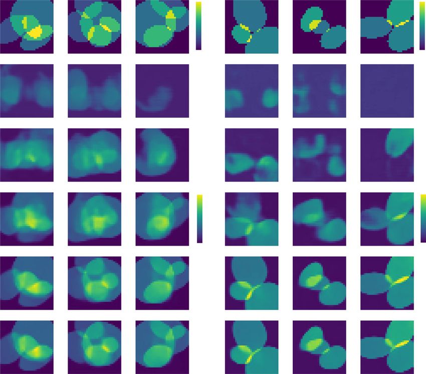
Kang et al. Light: Science & Applications (2021)10:74                                                            Page 2 of 21

obtained from the first order in the series expansion.           being considered and (2) the relationship of these priors to
Holographic approaches to volumetric reconstruction             the forward operator (Born, BPM, etc.) so as to produce a
generally rely on this first expansion term20–31. Often,         reasonable estimate of the inverse.
solving the Lippmann-Schwinger equation is the most                Here we propose a rather distinct approach to exploit
robust approach to account for multiple scattering, but         machine learning for a generic 3D refractive index
even then, the solution is iterative and requires excessive     reconstruction independent of the type of scattering. Our
amount of computation especially for complex 3D geo-            motivation is that, as the angle of illumination is changed,
metries. The inversion of these forward models to obtain        the light goes through the same scattering volume, but
the refractive index in 3D is referred to as inverse scat-      the scattering events, weak or strong, follow a different
tering, also a well-studied topic32–39.                         sequence. At the same time, the raw image obtained
  An alternative to the integral methods is the Beam            from a new angle of illumination adds information to the
Propagation Method (BPM), which sections the sample             tomographic problem, but that information is constrained
along the propagation distance z into slices, each slice        by (i.e. is not orthogonal to) the previously obtained
scattering according to the thin transparency model,            patterns. We interpret this as similar to a dynamical
and propagates the field from one slice to the next              system, where the output is constrained by the history of
through the object40. Despite some compromise in                earlier inputs as time evolves and new inputs arrive. (The
accuracy, BPM offers comparatively light load of com-           convolution integral is the simplest and best-known
putation and has been used as forward model for 3D              expression of this relationship between the output of a
reconstructions18. The analogy of the BPM computa-              system and the history of the system’s input.) An alter-
tional structure with a neural network was exploited, in        native interpretation is as dynamic programming51, where
conjunction with gradient descent optimization, to              the system at each step reacts so as to incrementally
obtain the 3D refractive index as the “weights” of the          improve an optimality criterion—in our case, the recon-
analogous neural network in the learning tomography             struction error metric.
approach41–43. BPM has also been used with more tra-               The analogy between tomography and a dynamical
ditional sparsity-based inverse methods33,44. Later, a          system suggests the RNN architecture as a strong candi-
machine learning approach with a Convolutional Neural           date to process raw images in sequence, as they are
Network (CNN) replacing the iterative gradient descent          obtained one after the other; and process them recur-
algorithm exhibited even better robustness to strong            rently so that each raw image from a new angle improves
scattering for layered objects, which match well with the       over the reconstructions obtained from the previous
BPM assumptions45. Despite great progress reported by           angles. Thus, we treat multiple raw images under different
these prior works, the problem of reconstruction                illumination angles as a temporal sequence, as shown in
through multiple scattering remains difficult due to the         Fig. 1. The angle index replaces what is a dynamical sys-
extreme ill-posedness and uncertainty in the forward            tem would have been the time t. This idea is intuitively
operator; residual distortion and artifacts are not             appealing; it also leads to considerable improvement in
uncommon in experimental reconstructions.                       the reconstructions, removing certain artifacts that were
  Inverse scattering, as inverse problems in general, may       visible in the strong scattering case of ref. 45.
be approached in a number of different ways to regularize          The dynamic reconstruction methodology applies, for
the ill-posedness and thus provide some immunity to             example, too weak scattering where the raw images are
noise46,47. Recently, thanks to a ground-breaking obser-        the sinograms; and too strong scattering, where the raw
vation from 2010 that sparsity can be learnt by a deep          images are better interpreted as intensity diffraction pat-
neural network48, the idea of using machine learning to         terns. The purpose of the learning scheme is to augment
approximate solutions to inverse problems also caught on        this relationship with regularization priors applicable to a
ref. 49. In the context of tomography, in particular, deep      certain class of objects of interest.
neural networks have been used to invert the Radon                 The way we propose to use RNNs in this problem is
transform50 and recursive Born model32, and were also the       quite distinct from the recurrent architecture proposed
basis of some of the papers we cited earlier on holographic     first in ref. 48 and subsequently implemented, replacing
3D reconstruction28–30, learning tomography41–43, and           the recurrence by a cascade of distinct neural networks, in
multi-layered strongly scattering objects45. In prior work      refs. 50,52,53, among others. In these prior works, the input
on tomography using machine learning, generally, the            to the recurrence can be thought of as clamped to the raw
intensity projections are all fed simultaneously as inputs to   measurement, as in the proximal gradient54 and related
a computational architecture that includes a neural net-        methods; whereas, in our case, the input to the recurrence
work, and the output is the 3D reconstruction of the            is itself dynamic, with the raw images from different
refractive index. The role of the neural network is to learn    angles forming the input sequence. Moreover, by utilizing
(1) the priors that apply to the particular class of objects    a modified gated recurrent unit (more on this below)
Dynamical machine learning volumetric reconstruction of objects' interiors from limited angular views
Kang et al. Light: Science & Applications (2021)10:74                                                                                 Page 3 of 21

                                                           N
                                                                                              g1

                                                     g le
                                                  An
                                                                 HN

                                             Angle n
                        Rotation of                                                                gn
                                                            Hn                                             Angular axis
                        illumination

                                                                 H1

                                                       1
                                                       gle
                                                                            f                 gN
                                                           An
 Fig. 1 Definition of the angular axis according to illumination angles. Each angle of illumination, here labeled as angular axis, corresponds to a
 time step in an analogous temporal axis

rather than a standard neural network, we do not need to                   used Radon transform assumption, i.e. weak scattering.
break the recurrence up into a cascade.                                    Then, we demonstrate the applicability of the dynamical
  Typical applications of RNNs55,56 are in temporal                        approach to strong scattering tomography. We show
sequence learning and identification. In imaging and                        significant improvement over static neural network-based
computer vision, RNN is applied in 2D and 3D: video                        reconstructions of the same experimental data under the
frame prediction57–60, depth map prediction61, shape                       strong scattering assumption. The improvement is shown
inpainting62; and stereo reconstruction63,64 or segmenta-                  both visually and in terms of several quantitative metrics.
tion65,66 from multi-view images, respectively. Stereo, in                 Results from an ablation study indicate the relative sig-
particular, bears certain similarities to our tomographic                  nificance of the new components we introduced to the
problem here, as sequential multiple views can be treated                  quality of the reconstructions.
as a temporal sequence. To establish the surface shape,
the RNNs in these prior works learn to enforce con-                        Results
sistency in the raw 2D images from each view and resolve                      Our first investigation of the recurrent reconstruction
the redundancy between adjacent views in recursive                         scheme is for weak scattering, i.e. when the Radon trans-
fashion through the time sequence (i.e. the sequence of                    form approximation applies and with a limited range of
view angles). Non-RNN learning approaches have also                        available angles. For simulation, each sample consists of
been used in stereo, e.g. Gaussian mixture models67. In                    random number, between 1 and 5 with equal probability, of
computed tomography, in particular, an alternate dyna-                     ellipsoids at random locations with arbitrarily chosen sizes,
mical neural network of the Hopfield type has been used                     amplitudes, and angles, thus spatially isotropic in average.
successfully68.                                                            Rotation is applied along the x-axis, from −10° to +10° with
  In this work, we replaced the standard Long Short-                       1° increment, thus 21 projections per sample under a
Term Memory (LSTM)56 implementation of RNNs with a                         parallel-beam geometry. The Filtered Backprojection (FBP)
modified version of the newer Gated Recurrent Unit                          algorithm3 is used to generate crude estimates from the
(GRU)69. The GRU has the advantage of fewer parameters                     projections. nth FBP Approximant (n = 1,2,…,21) is the
but generalizes comparably with the LSTM. Our GRU                          reconstruction by the FBP algorithm using n projections of
employs a separable-convolution scheme to explicitly                       n angles starting from −10°.
account for the asymmetry between the lateral and axial                       The reconstructions by the RNN are compared in Fig. 2
axes of propagation. We also utilize an angular attention                  with FBP and Total Variation (TV)-regularized recon-
mechanism whose purpose is to learn how to reward                          structions using TwIST71 for qualitative and visual com-
specific angles in proportion to their contribution to                      parison. Here a TV-regularization parameter is set to be
reconstruction quality70. We found that for the strongly                   0.01, and the algorithm is run up to 200 iterations until its
anisotropic samples or scanning schemes the angular                        objective function saturates. Figure 3 shows the quanti-
attention mechanism is effective.                                          tative comparison on test performance using three dif-
  The results of our simulation and experimental study on                  ferent quantitative metrics, where FBP and FBP + TV
a generic interior volumetric reconstruction are in                        yielded much lower values than the recurrent scheme.
Results. We first show numerically that the dynamical                          Figure 4 shows the evolution of test reconstructions as new
machine learning approach is suitable to tomographic                       projections or FBP Approximants are presented to the
reconstruction under more restrictive and commonly                         dynamical scheme. When the recurrence starts with n = 1,
Dynamical machine learning volumetric reconstruction of objects' interiors from limited angular views
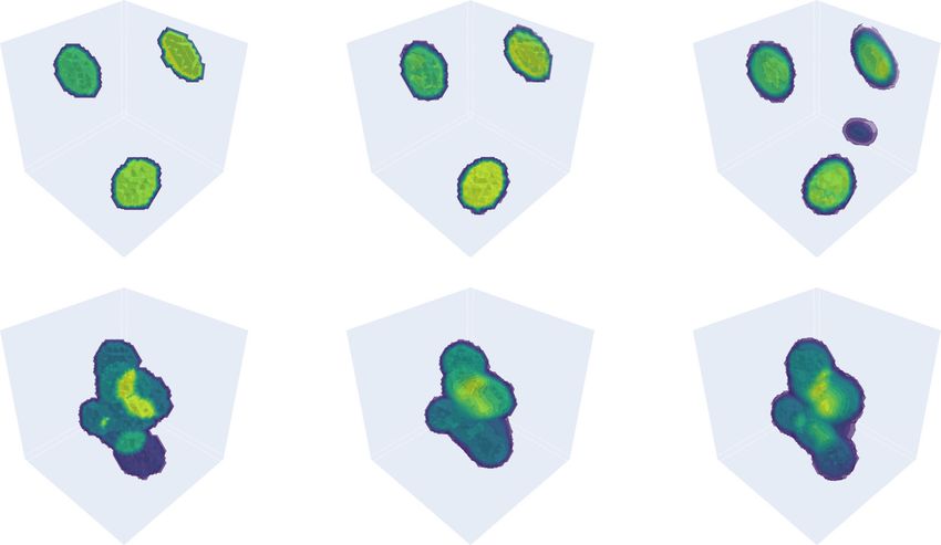
Kang et al. Light: Science & Applications (2021)10:74                                                                                                                Page 4 of 21

                             Sample 1                                                                                                                Sample 2
                        xz       yz                             xy                           xz                                                           yz    xy
                                                                     2.72                                                                                                   1.62
   Ground truth

                                                                            Amplitude

                                                                                                                                                                                  Amplitude
                                                                     0                                                                                                     0

                                                                     0.876                                                                                                  0.432

                                                                            Amplitude

                                                                                                                                                                                  Amplitude
   FBP

                                                                     –1.29                                                                                                  –0.893

                                                                     0.921                                                                                                  0.514
   FBP + TV

                                                                            Amplitude

                                                                                                                                                                                  Amplitude
                                                                     –1.32                                                                                                  –0.994

                                                                     2.54                                                                                                   1.60
   Proposed RNN

                                                                            Amplitude

                                                                                                                                                                                  Amplitude
                                                                     –0.027                                                                                                 –0.065

                                                                     G.T.                                                                                                  G.T.
                                                                     FBP                                                                                                   FBP
                                                                     FBP + TV                                                                                              FBP + TV
                                                                     RNN                                                                                                   RNN

 Fig. 2 Dynamic approach for projection tomography (i.e. subject to the Radon transform approximation) using simulated data. Each
 simulated sample contains randomly generated ellipsoids. Shown are xz, yz, and xy cross-sections of ground truth and reconstructions by Filtered
 Backprojection (FBP), TV-regularized Filtered Backprojection (FBP + TV), and the proposed RNN. Red dashed lines show where the 1D cross-section
 profiles are drawn

                  1.0                                         1.0                                                                                    30
                                      Proposed RNN                                                Proposed RNN
                                      FBP + TV                                                    FBP + TV
                                      FBP                                                         FBP
                  0.9                                                                                                                                25
                                                              0.8
                                                                                                                 Wasserstein distance (x 0.01) ( )

                  0.8                                                                                                                                20
                                                              0.6
                                                     )
   )

                                                     SSIM (
   PCC (

                  0.7                                                                                                                                15

                                                              0.4
                  0.6                                                                                                                                10

                                                              0.2
                  0.5                                                                                                                                 5
                                                                                                                                                                     Proposed RNN
                                                                                                                                                                     FBP + TV
                                                                                                                                                                     FBP
                  0.4                                         0.0                                                                                     0

 Fig. 3 Test performance under the weak scattering condition. The figure quantitatively compares the recurrent scheme with FBP + TV, and FBP.
 The graphs show the means and 95% confidence intervals

the volumetric reconstruction is quite poor; as more projec-                              Details of the recurrent architecture for the weak
tions are included, the reconstruction improves as expected. It                         scattering assumption are presented in Fig. 16b. To
is also interesting to see that not all the angles are needed to                        quantify the relative contributions to reconstruction
achieve reasonable quality of reconstructions as the graphs                             quality of each element in the architecture, the elements
and reconstructions in Fig. 4a, b saturate around n = 19.                               one by one are ablated (-) or substituted ($) with
Dynamical machine learning volumetric reconstruction of objects' interiors from limited angular views
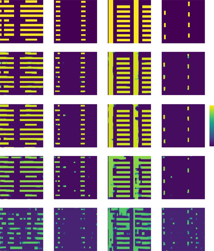
Kang et al. Light: Science & Applications (2021)10:74                                                                                                                         Page 5 of 21

   a                                                                                           b                   Sample 1                                   Sample 2
                                                                                                              xz      yz         xy                      xz     yz       xy
                                         0.9                                                                                             2.72                                       1.62

                                                                                               Ground truth
                                         0.8

                                                                                                                                             Amplitude

                                                                                                                                                                                        Amplitude
                                         0.7
   )
   PCC (

                                         0.6                                                                                             0                                          0

                                         0.5

                                         0.4

                                                                                               n=1
                                         0.3                                            PCC

                                               1   5   9         13          17           21
                                                           n

                                         0.8

                                                                                               n=7
                                         0.7
                                         0.6
   )

                                         0.5
   SSIM (

                                                                                                                                         2.54                                       1.60

                                         0.4                                                   n = 13

                                                                                                                                                                                        Amplitude
                                                                                                                                             Amplitude
                                         0.3
                                         0.2
                                                                                                                                                                                    –0.065
                                         0.1                                           SSIM
                                                                                                                                         –0.027

                                               1   5   9         13          17           21
                                                           n
                                                                                               n = 19

                                                               Wasserstein distance (× 0.01)
     Wasserstein distance (× 0.01) ( )

                                         25

                                         20
                                                                                               n = 21

                                         15

                                         10
                                                                                                                                         G.T.                                       G.T.
                                                                                                                                         n=1                                        n=1
                                                                                                                                         n=7                                        n=7
                                          5                                                                                              n = 13                                     n = 13
                                                                                                                                         n = 19                                     n = 19
                                               1   5   9         13          17           21                                             n = 21                                     n = 21

                                                           n

 Fig. 4 Progression of 3D reconstruction performance under the weak scattering condition. a Three quantitative metrics are used to quantify
 test performance of the trained recurrent neural network under the weak scattering assumption using simulated data, i.e. Pearson Correlation
 Coefficient (PCC), Structural Similarity Index Metric (SSIM), and Wasserstein distance. b Progression of 3D reconstruction performance as the FBP
 Approximants n ¼ 1; ¼ ; Nð¼ 21Þ are projected to the recurrent scheme. Movies as Supplementary movies 1 and 2 show the progression of the
 reconstructions of Samples 1 and 2, respectively. Red dashed lines show where the 1D cross-section profiles are drawn

alternatives. This ablation study is performed on a                                                                   tomographic reconstructions under the weak scattering
strategy to giving weights on hidden features, separable                                                              assumption. However, for the ablation of the angular
convolution, and ReLU (rectified linear unit) activation                                                               attention mechanism, it makes no large difference from the
function72 inside the recurrence cell. Specifically, in the                                                            performance of the proposed model, which is because
study, (1) an angular attention mechanism is ablated, or                                                              the objects used for training and testing are isotropic in
only last hidden feature hn is taken into account before                                                              average and do not show any preferential direction.
the decoder instead of the angular attention mechanism;                                                                 Here, we perform an additional study on the role of the
(2) a separable convolution scheme is ablated, thus the                                                               angular attention mechanism by granting a preferential
standard 3D convolution; and (3) ReLU activation                                                                      direction or spatial anisotropy to the objects of interest. In
function is ablated and then substituted with the tanh                                                                this study, the mean major axis of the objects is assumed
activation function, which is more usual69. The ablated                                                               to be parallel to the z-axis, i.e. the objects are elongated
architectures are trained under the same training                                                                     along the axis. Instead of the previously examined sym-
scheme (for more details, see Training the recurrent                                                                  metric angular scanning range (−10°, +10°), we now
neural network in Materials and methods) and tested                                                                   consider the asymmetric case (−15°, +5°).
with the same simulated data.                                                                                           In Fig. 7a, the angular attention with the asymmetry now
  Visually, in Fig. 5, test performance largely degrades as the                                                       gives attention on n differently, i.e. its peak translated to the
ablation happens on the ReLU activation function and                                                                  left by 5. It is because the projections from higher angles
separable convolution, which is also found quantitatively in                                                          may contain more useful information on the objects due to
Fig. 6. Therefore, for the Radon case, we find that (1) ReLU                                                           the directional preference of the objects, thus the distribu-
activation function is highly desirable instead of the native                                                         tion of the attention probabilities is now attracted to
tanh function; (2) the separable convolution is helpful                                                               the lower indices. In Fig. 7b, we quantitatively show that the
when designing a recurrent unit and encoder/decoder for                                                               angular attention improves performance in the case of the
Dynamical machine learning volumetric reconstruction of objects' interiors from limited angular views
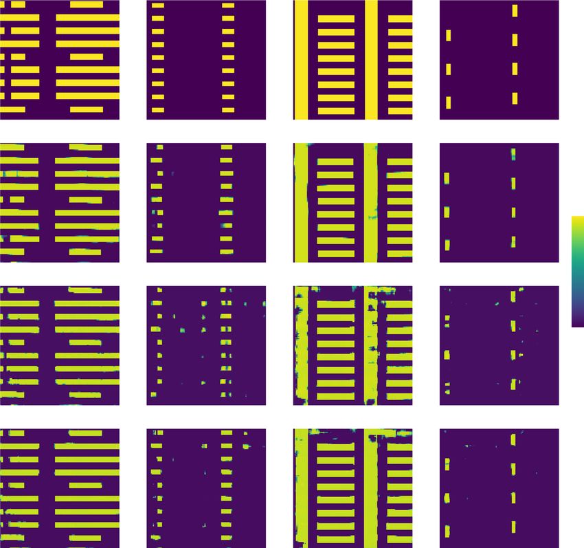
Kang et al. Light: Science & Applications (2021)10:74                                                                                                                                           Page 6 of 21

                                           Sample 1                                                                                                                       Sample 2
                                     xz         yz                                xy                              xz                                                          yz     xy
             Ground truth
             Proposed RNN

                                                                                       2.54                                                                                                               1.69
             (–) angular attention

                                                                                           Amplitude

                                                                                                                                                                                                              Amplitude
                                                                                       0                                                                                                                  0
      (–) separable
       convolution
             ( ) tanh

 Fig. 5 Ablation study on the recurrent architecture under the weak scattering condition. Qualitative representations are shown when some
 elements of the recurrent architecture in Fig. 16b are ablated, and the rows are ordered by increasing severity of the ablation effects according to Fig. 6

           0.98                                                                0.90                                                                                       9

                                                                                                                                                                          8
                                                                               0.85
           0.96
                                                                                                                                                                          7
                                                                                                                                      Wasserstein distance (x 0.01) ( )

                                                                               0.80
                                                                                                                                                                          6
           0.94
                                                                               0.75
                                                                      )
   )

                                                                                                                                                                          5
                                                                      SSIM (
   PCC (

                                                                               0.70                                                                                       4
           0.92
                                                                                                                                                                          3
                                                                               0.65
                                                                                                                                                                          2
           0.90                           Proposed RNN                                                    Proposed RNN                                                                Proposed RNN
                                          (–) Angular attention                0.60                       (–) Angular attention                                                       (–) Angular attention
                                          (–) Separable convolution                                       (–) Separable convolution                                       1           (–) Separable convolution
                                          ( ) tanh                                                        ( ) tanh                                                                    ( ) tanh
           0.88                                                                0.55                                                                                       0

 Fig. 6 Quantitative analysis on test performance in the ablation study under the weak scattering condition. The graphs show the means and
 95% confidence intervals

asymmetric scanning of objects with directionality regard-                                             and methods” for details). Networks trained with exam-
less of the noise present in projections.                                                              ples with small and dense features tend to generalize
  Figures 8 and 9 characterize our proposed method in                                                  better and with less artifacts than large and sparse fea-
terms of feature size and feature sparsity, as well as cross-                                          tures, in agreement with ref. 73. Lastly, and not surpris-
domain generalization, compared to the baseline model                                                  ingly, overall reconstruction quality is better when feature
(see Training the recurrent neural network in “Materials                                               size is large and features are sparse.
Dynamical machine learning volumetric reconstruction of objects' interiors from limited angular views
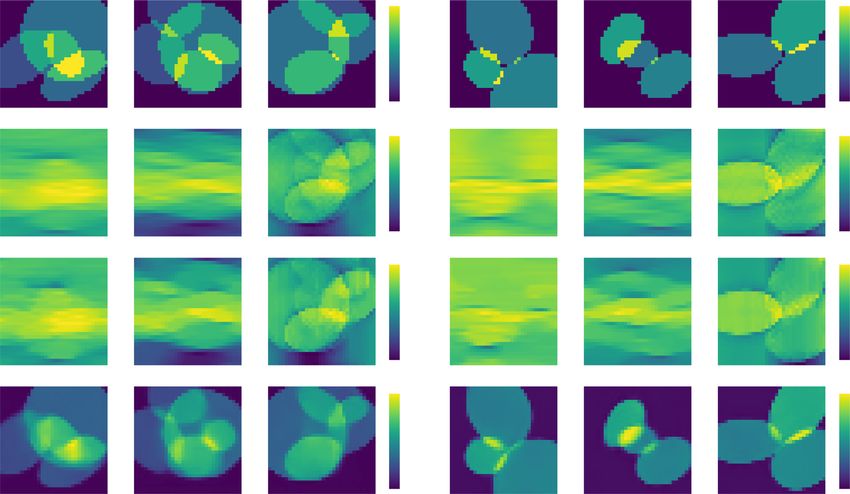
Kang et al. Light: Science & Applications (2021)10:74                                                                                                                                                                                                                                                                                                                                                                  Page 7 of 21

      a                                                                                                         b         0.980                                                                                                  0.97                                                                                                                              1.6
                                      0.050

                                                                                                                          0.975                                                                                                  0.96
                                      0.049                                                                                                                                                                                                                                                                                                                        1.4

                                                                                                                                                                                                                                                                                                                               Wasserstein distance (x 0.01) ( )
       Attention probabilities (n)

                                      0.048                                                                               0.970                                                                                                  0.95

                                                                                                                                                                                                                                                                                                                                                                   1.2

                                                                                                                                                                                                                     SSIM ( )
                                                                                                                PCC ( )
                                      0.047                                                                               0.965                                                                                                  0.94

                                                                                                                                                                                                                                                                                                                                                                   1.0
                                      0.046                                                                               0.960                                                                                                  0.93

                                      0.045                                                                                                                                                                                                                                                                                                                        0.8
                                                                                                                          0.955                                                                                                  0.92

                                                                             Scanning range: (–10°, +10°)                                                                                     With attention                                                                                           With attention                                                                                                       With attention
                                      0.044                                  Scanning range: (–15°, +5°)                                                                                      Without attention                                                                                        Without attention                                                                                                    Without attention
                                                                                                                          0.950                                                                                                  0.91                                                                                                                              0.6
                                                1 2 3 4 5 6 7 8 9 10 11 12 13 14 15 16 17 18 19 20 21                             Noiseless                 100 photons/pixel    Noiseless    100 photons/pixel                         Noiseless     100 photons/pixel           Noiseless            100 photons/pixel                                                 Noiseless     100 photons/pixel       Noiseless     100 photons/pixel
                                                                         n                                                                       Scanning range: (–10°, +10°)       Scanning range: (–15°, +5°)                            Scanning range: (–10°, +10°)               Scanning range: (–15°, +5°)                                                           Scanning range: (–10°, +10°)          Scanning range: (–15°, +5°)

 Fig. 7 Attention probabilities and angular attention mechanism for different ranges of scanning. a Attention probabilities according to
 different ranges of scanning. Here, for the scanning range of (−10°, +10°), n = 1 and 21 correspond to −10° and +10°, respectively; and for the
 scanning range of (−15°, +5°), they correspond to −15° and +5°, respectively. b Test performance for our examined scanning ranges with and
 without the angular attention mechanism. The graphs show the means and 95% confidence intervals

  a                                    0.98
                                                                                                                                  b                                                                                                                                                  c
                                                                                      Baseline (21 M)                                                                                                                                                         0.96                                                                                                                                                                       0.96
                                                                                      Proposed RNN (21 M)
                                       0.97
                                                                                                                                                                                                                                                              0.94                                                                                                                                                                       0.94
                                       0.96                                                                                                        Small               0.9192 ± 0.0069                            0.8705 ± 0.0094                                                                   Small            0.9368 ± 0.0030                                                       0.9064 ± 0.0058
                                                                                                                                                                                                                                                              0.92                                                                                                                                                                       0.92
                                       0.95
                                                                                                                                  Trained with

                                                                                                                                                                                                                                                                                     Trained with
      )

                                                                                                                                                                                                                                                                          )

                                                                                                                                                                                                                                                                                                                                                                                                                                                 )
                                                                                                                                                                                                                                                              0.90                                                                                                                                                                       0.90
      PCC (

                                                                                                                                                                                                                                                                          PCC (

                                                                                                                                                                                                                                                                                                                                                                                                                                                 PCC (
                                       0.94
                                                                                                                                                                                                                                                              0.88                                                                                                                                                                       0.88
                                       0.93
                                                                                                                                                                                                                                                              0.86                                                                                                                                                                       0.86
                                       0.92                                                                                                        Large               0.8218 ± 0.0127                            0.9578 ± 0.0023                                                                   Large           0.8246 ± 0.0099                                                         0.9632 ± 0.0016
                                                                                                                                                                                                                                                              0.84                                                                                                                                                                       0.84
                                       0.91
                                                                                                                                                                                                                                                              0.82                                                                                                                                                                       0.82
                                       0.90
                                                              Small                                Large                                                                        Small                                           Large                                                                                          Small                                                                Large
                                                                                                                                                                                               Tested with                                                                                                                                                               Tested with

  d                                                                                                                                                                                                                                                              Tested with
                                                                      Ground truth                                                                                                                         Small                                                                                                                                                          Large
                                        Small

                                                 z                                                                                                                    z                                                                                                                                 z
   Trained with

                                                               y                                            x                                                                           y                                                  x                                                                               y                                                                               x
                                        Large

                                                 z                                                                                                                    z                                                                                                                                 z

                                                               y                                            x                                                                           y                                                  x                                                                               y                                                                               x

 Fig. 8 Sample feature size and testing performance. a Quantitative comparison of testing performance in terms of feature size, and cross-domain
 generalization result of (b) the baseline model (21 M) and (c) the proposed RNN (21 M). d Qualitative comparison of a volumetric reconstruction for
 different cases of training and testing conditions in terms of feature size (see Table S1 in Supplementary Information (SI) Section S1 for more details)
Dynamical machine learning volumetric reconstruction of objects' interiors from limited angular views
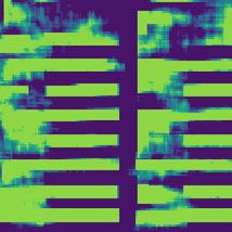
Kang et al. Light: Science & Applications (2021)10:74                                                                                                                                                                                Page 8 of 21

   a               0.96
                                                                      b                                                                                        c
                                                Baseline (21 M)
                                                Proposed RNN (21 M)
                                                                                                                                                0.92                                                                                     0.92
                   0.94
                                                                                     Sparse       0.9203 ± 0.0089             0.8190 ± 0.0102                                 Sparse   0.9329 ± 0.0053             0.8557 ± 0.0052
                                                                                                                                                0.90                                                                                     0.90

                   0.92

                                                                                                                                                               Trained with
                                                                      Trained with
         )

                                                                                                                                                                                                                                                )
                                                                                                                                                       )
                                                                                                                                                0.88                                                                                     0.88

                                                                                                                                                                                                                                                PCC (
         PCC (

                                                                                                                                                       PCC (
                   0.90
                                                                                                                                                0.86                                                                                     0.86

                                                                                     Dense        0.8576 ± 0.0157             0.8871 ± 0.0067                                 Dense    0.9017 ± 0.0062             0.9161 ± 0.0031
                                                                                                                                                0.84                                                                                     0.84
                   0.88

                                                                                                                                                0.82                                                                                     0.82
                   0.86
                                                                                                      Sparse                      Dense                                                    Sparse                      Dense
                                Sparse                Dense
                                                                                                                Tested with                                                                          Tested with

   d                                                                                                                                              Tested with
                                         Ground truth                                                                Sparse                                                                          Dense
                  Sparse

                            z                                                                 z                                                                                   z
   Trained with

                                 y                         x                                               y                                x                                              y                                x
                    Dense

                            z                                                                 z                                                                                   z

                                 y                         x                                               y                                x                                              y                                x

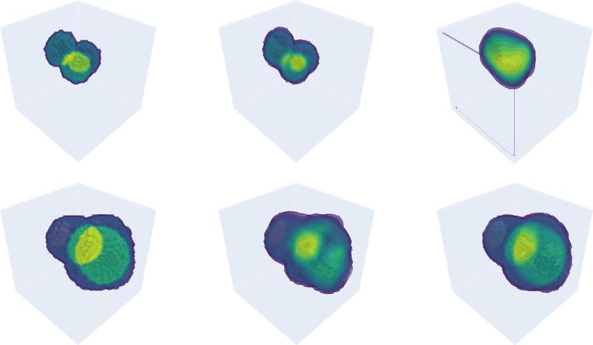
 Fig. 9 Sample sparsity and testing performance. a Quantitative comparison of testing performance in terms of sparsity, and cross-domain
 generalization result of (b) the baseline model (21 M) and (c) the proposed RNN (21 M). d Qualitative comparison of a volumetric reconstruction for
 different cases of training and testing conditions in terms of sparsity. For more details, see Table S1 in SI Section S1

  Next, we investigate the case when the Radon transform                                                                         more details in the DWMA process. The evolution of the
is not applicable, i.e. tomography under strong scattering                                                                       RNN output as more DWMA Approximants are pre-
conditions and under a similarly limited-angle scheme.                                                                           sented is shown in Fig. 10 and shows a similar improve-
The RNN is first trained with the single-pass, gradient                                                                           ment with recurrence m as in the Radon case of Fig. 4.
descent-based Approximants Eq. (4) of simulated dif-                                                                             Also, like the Radon case, it is interesting to see that not
fraction patterns (see Training and testing procedures in                                                                        all the Approximants are needed to acquire reasonable
Materials and methods), and then tested with the simu-                                                                           quality of reconstructions: the graphs in Fig. 10a saturate
lated ones and additionally with the TV-based Approx-                                                                            around m = 10 and the visual quality of the reconstruc-
imants Eq. (5) of experimentally obtained diffraction                                                                            tions at m = 10–12 in Fig. 10b does not largely differ.
patterns. TV regularization is only applied to the                                                                                 For comparison, the 3D-DenseNet architecture with skip
experimental patterns. To reconcile any experimental                                                                             connections in ref. 45 and its modified version with more
artifacts, there is an additional step of Dynamic Weighted                                                                       parameters to match with that of our RNN are set as
Moving Average (DWMA) on the Approximants                                                                                        baseline models (see Training the recurrent neural network
f n½1 ðn ¼ 1; 2; ¼ ; 42Þ, hence DWMA Approximants                                                                               in Materials and methods for details). Our RNN has
  ½1
                                                                                                                                 approximately 21 M parameters, and visual comparisons
f~m ðm ¼ 1; 2; ¼ ; 12Þ. See “Materials and methods” for                                                                          with the baseline 3D-DenseNets with 0.5 M and 21 M
Dynamical machine learning volumetric reconstruction of objects' interiors from limited angular views
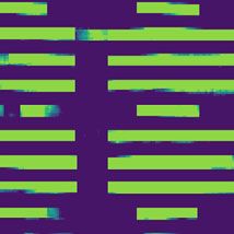
Kang et al. Light: Science & Applications (2021)10:74                                                                                                                                               Page 9 of 21

   a                                                                                                                      b              Layer 1          Layer 2         Layer 3         Layer 4
                                         1.0
                                                                                                                                                                                                       5.24

                                                                                                                          Ground truth
                                         0.9

                                                                                                                                                                                                              Δn (x 10-2)
                                         0.8
   PCC ( )

                                                                                                                                                                                                       2.62
                                         0.7

                                         0.6

                                         0.5                                                                                                                                                           0
                                                                                                     PCC (Simulation)
                                         0.4                                                         PCC (Experiment)

                                               1   2   3   4   5   6         7      8       9       10      11      12
                                                                       m

                                                                                                                          m=1
                                         1.0

                                         0.9

                                         0.8
   SSIM ( )

                                         0.7

                                         0.6

                                         0.5

                                         0.4                                                        SSIM (Simulation)
                                                                                                    SSIM (Experiment)
                                         0.3                                                                              m=5
                                               1   2   3   4   5   6         7      8       9       10      11      12
                                                                       m
                                                                                                                                                                                                       5.06
     Wasserstein distance (x 0.01) ( )

                                                                           Wasserstein distance (x 0.01) (Simulation)
                                         10                                Wasserstein distance (x 0.01) (Experiment)

                                                                                                                                                                                                              Δn (x 10-2)
                                          8
                                                                                                                                                                                                       2.53
                                          6

                                          4
                                                                                                                                                                                                       0
                                                                                                                          m = 10

                                          2

                                          0
                                               1   2   3   4   5   6         7      8       9       10      11      12
                                                                       m

                                         14                                       Probability of error (%) (Simulation)
                                                                                  Probability of error (%) (Experiment)
     Probability of error (%) ( )

                                         12

                                         10

                                          8
                                                                                                                          m = 12

                                          6

                                          4

                                          2

                                          0
                                               1   2   3   4   5   6         7      8       9       10      11      12
                                                                       m

 Fig. 10 Progress of 3D reconstruction performance as diffraction patterns from different angles are presented to the recurrent scheme.
                                ½1
 Here, DWMA Approximants ~f m ðm ¼ 1; 2; ¼ ; 12Þ are presented to the RNN sequentially. a Four quantitative metrics (PCC, SSIM, Wasserstein
 distance, and Probability of Error; PE) quantitatively show the progress using both simulated and the experimental data. The graphs show the mean
 of the metrics of Layers 1–4. b Qualitative comparison using experimental data with different m = 1, 5, 10, and 12

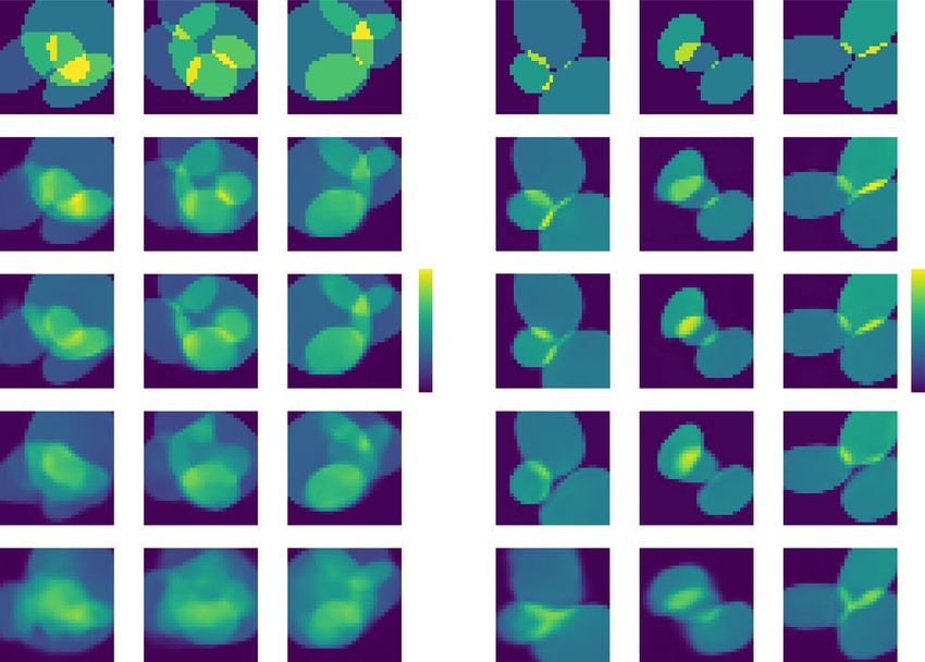
parameters are shown in Fig. 11. The RNN results show                                                                                                Visually in Fig. 13, unlike the Radon case, paying
substantial visual improvement, with fewer artifacts and                                                                                           attention only to the last hidden feature affects and
distortions compared to the static approaches of ref. 45, even                                                                                     degrades the testing performance worst. Also, it is
when the number of parameters in the latter matches ours.                                                                                          important to note that the ablation of the separable
PCC, SSIM, Wasserstein distance, and PE are used to                                                                                                convolution scheme brings degradation in test perfor-
quantify test performance using simulated and experimental                                                                                         mance according to Fig. 13. The decrease in test perfor-
data in Fig. 12.                                                                                                                                   mance by the substitution of ReLU with the more
  We also conducted an ablation study of the learning                                                                                              common tanh is comparatively marginal. These findings
architecture of Fig. 16d. Similar to the Radon case, each                                                                                          are supported quantitatively as well in Fig. 14.
component in the architecture was ablated or substituted                                                                                             Thus, under the strong scattering condition, we find that
with its alternative, one at a time: (1) ReLU was ablated                                                                                          (1) hidden features from all angular steps need to be taken
and then substituted with the native tanh activation                                                                                               into consideration with the angular attention mechanism for
function, (2) the separable convolution was ablated, thus                                                                                          reconstructions to get a better test performance although
the standard 3D convolution, and (3) the angular atten-                                                                                            the last hidden feature is assumed to be informed of the
tion mechanism was ablated, or only the last hidden                                                                                                history of the previous angular steps; (2) replacing the
feature was given attention. The ablated architectures are                                                                                         standard 3D convolution with the separable convolution
also trained under the same training scheme (see Training                                                                                          helps when designing a recurrent unit and a convolutional
the recurrent neural network in “Materials and methods”                                                                                            encoder/decoder for tomographic reconstructions; and (3)
for more details) and tested with both the simulated                                                                                               the substitution of tanh with ReLU is still useful but may be
Eq. (4) and experimental Approximants Eq. (5).                                                                                                     application dependent.
Dynamical machine learning volumetric reconstruction of objects' interiors from limited angular views
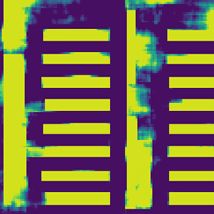
Kang et al. Light: Science & Applications (2021)10:74                                                                                                                                                                                                                                                                                           Page 10 of 21

                                                           Layer 1                                              Layer 2                                                                  Layer 3                                    Layer 4

                                     Ground truth
                                     Proposed RNN (21 M)

                                                                                                                                                                                                                                                                                                                         5.24

                                                                                                                                                                                                                                                                                                                                  Δn (× 10–2)
                                     Baseline (0.5 M)

                                                                                                                                                                                                                                                                                                                         0
                                     Baseline (21 M)

 Fig. 11 Qualitative comparison on test performance between the baseline and proposed architectures using experimental data. The
 baseline architectures are 3D-DenseNet CNN architectures with 0.5 M and 21 M parameters. Our proposed architecture is a recurrent neural network
 with elements (for more details, see Computational architecture in Materials and methods)

   a 1.000                                                                                    1.000
                                                                                                                                                                                              0.6                           Proposed RNN                                                                                                        Proposed RNN
                                                                                                                                                                                                                                                                                               0.40
                  0.998                                                                                                                                                                                                     Baseline (0.5 M)                                                                                                    Baseline (0.5 M)
                                                                                              0.998
                                                                                                                                                          Wasserstein distance (x 0.01) ( )

                                                                                                                                                                                                                            Baseline (21 M)                                                    0.35                                             Baseline (21 M)
                                                                                                                                                                                              0.5
                                                                                                                                                                                                                                               Probability of error (%) ( )

                  0.996
                                                                                              0.996                                                                                                                                                                                            0.30
                  0.994                                                                                                                                                                       0.4
                                                                              SSIM ( )
   PCC ( )

                                                                                                                                                                                                                                                                                               0.25
                                                                                              0.994
                  0.992                                                                                                                                                                       0.3                                                                                              0.20

                  0.990                                                                       0.992                                                                                                                                                                                            0.15
                                                                                                                                                                                              0.2
                                                                                                                                                                                                                                                                                               0.10
                  0.988                                    Proposed RNN                                                          Proposed RNN
                                                                                              0.990                                                                                           0.1
                                                           Baseline (0.5 M)                                                      Baseline (0.5 M)                                                                                                                                              0.05
                  0.986                                    Baseline (21 M)                                                       Baseline (21 M)
                                                                                              0.988                                                                                           0.0                                                                                              0.00
                             Layer 1 Layer 2 Layer 3 Layer 4 Overall                                      Layer 1 Layer 2 Layer 3 Layer 4 Overall                                                   Layer 1 Layer 2 Layer 3 Layer 4 Overall                                                                      Layer 1 Layer 2 Layer 3 Layer 4 Overall

   b                   1.0                                                                          0.9
                                                                                                                                                                                              3.0                                                                                                            7
                       0.9                                                                          0.8
                                                                                                                                                     Wasserstein distance (x 0.01) ( )

                                                                                                                                                                                              2.5                                                                                                            6
                                                                                                                                                                                                                                                                              Probability of error (%) ( )

                       0.8
                                                                                                    0.7                                                                                                                                                                                                      5
                                                                                                                                                                                              2.0
                                                                                         SSIM ( )

                       0.7
             PCC ( )

                                                                                                                                                                                                                                                                                                             4
                                                                                                    0.6
                                                                                                                                                                                              1.5
                       0.6
                                                                                                                                                                                                                                                                                                             3
                                                                                                    0.5                                                                                       1.0
                       0.5                                                                                                                                                                                                                                                                                   2
                                                           Proposed RNN                                                           Proposed RNN                                                          Proposed RNN                                                                                                 Proposed RNN
                       0.4                                                                          0.4                                                                                       0.5
                                                           Baseline (0.5 M)                                                       Baseline (0.5 M)                                                      Baseline (0.5 M)                                                                                     1       Baseline (0.5 M)
                                                           Baseline (21 M)                                                        Baseline (21 M)                                                       Baseline (21 M)                                                                                              Baseline (21 M)
                       0.3                                                                          0.3                                                                                       0.0                                                                                                            0
                             Layer 1 Layer 2 Layer 3 Layer 4 Overall                                      Layer 1 Layer 2 Layer 3 Layer 4 Overall                                                   Layer 1 Layer 2 Layer 3 Layer 4 Overall                                                                      Layer 1 Layer 2 Layer 3 Layer 4 Overall

 Fig. 12 Test performance on simulated and experimental data under the strong scattering condition. For the quantitative comparison, four
 different metrics are used, i.e. PCC, SSIM, Wasserstein distance, and PE on (a) simulated and (b) experimental data. Graphs in (a) show the means and
 95% confidence intervals. Raw data of Fig. 12b can be found in Table S2 in SI Section S2
Kang et al. Light: Science & Applications (2021)10:74                                                                                           Page 11 of 21

                                               Layer 1   Layer 2              Layer 3                   Layer 4

                       Ground truth
                       Proposed RNN

                                                                                                                           5.24
                       ( ) tanh

                                                                                                                                  Δn (x 10-2)
                                                                                                                           0
                (–) separable
                 convolution
                       (–) angular attention

 Fig. 13 Visual quality assessment from the ablation study on elements (see “Computational architecture in Materials and methods” for
 details) using experimental data. Rows 3–5 show reconstructions based on experimental data for each layer upon the ablation and substitution of
 ReLU activation in Eq. (10) with the more common tanh activation function instead (row 3); ablating the separable convolution scheme, thus the
 standard 3D convolution (row 4); ablating the angular attention mechanism and putting attention to only last hidden feature (row 5). The rows are
 ordered by increasing severity of the ablation effect according to Fig. 14b

Discussion                                                                 the reconstructions. We found that the angular attention
   We have proposed a new recurrent neural network scheme                  mechanism takes an important role especially when the
for a generic interior-volumetric reconstruction by processing             objects of interest are spatially anisotropic and performs
raw inputs from different angles of illumination dynamically,              better than placing all the attention on only the last hid-
i.e. as a sequence, with each new angle improving the 3D                   den feature. Even though the last hidden feature is a
reconstruction. We found this approach to work well under                  nonlinear multivariate function of all the previous hidden
two types of scattering assumptions: weak (Radon transform)                features, as it has a propensity to reward the latter
and strong. In the second case, in particular, we observed                 representations but the former ones74, the last hidden
significant qualitative and quantitative improvement over the               feature may not sufficiently represent all angular views.
static machine learning scheme of ref. 45, where the raw inputs            Hence, the angular attention mechanism adaptively
from all angles are processed at once by a neural network.                 merges information from all angles. This is particularly
   Through the ablation studies, we found that sand-                       important for our strong scattering case as each DWMA
wiching the recurrent structure with some key elements                     Approximant involves a diffraction pattern of a certain
between a convolutional encoder/decoder helps improve                      illumination angle; whereas an FBP Approximant under
Kang et al. Light: Science & Applications (2021)10:74                                                                                                                                                                                                                                                                                                                                            Page 12 of 21

    a               1.000                                                                        1.0000
                                                                                                                                                                                                                                                  Proposed RNN                                                                                             Proposed RNN
                                                                                                                                                                                                                                          0.5     ( ) tanh                                                                                         0.5     ( ) tanh
                                                                                                 0.9975                                                                                                                                           (–) Separable convolution                                                                                (–) Separable convolution
                    0.995
                                                                                                                                                                                                                                                  (–) Angular attention                                                                                    (–) Angular attention

                                                                                                 0.9950
                                                                                                                                                                                                                                          0.4                                                                                                      0.4

                                                                                                                                                                               Wasserstein distance (x 0.01) ( )
                    0.990

                                                                                                                                                                                                                                                                                                               Probability of error (%) ( )
                                                                                                 0.9925
                    0.985

                                                                                    SSIM ( )
    PCC ( )

                                                                                                                                                                                                                                          0.3                                                                                                      0.3
                                                                                                 0.9900

                    0.980
                                                                                                 0.9875                                                                                                                                   0.2                                                                                                      0.2

                    0.975
                                                                                                 0.9850
                               Proposed RNN                                                                       Proposed RNN                                                                                                            0.1                                                                                                      0.1
                    0.970      ( ) tanh                                                                           ( ) tanh
                                                                                                 0.9825
                               (–) Separable convolution                                                          (–) Separable convolution
                               (–) Angular attention                                                              (–) Angular attention
                    0.965                                                                        0.9800                                                                                                                                   0.0                                                                                                      0.0
                            Layer 1      Layer 2      Layer 3   Layer 4   Overall                               Layer 1     Layer 2      Layer 3       Layer 4      Overall                                                                     Layer 1     Layer 2      Layer 3       Layer 4       Overall                                             Layer 1     Layer 2      Layer 3       Layer 4       Overall

    b                1.0                                                                                  1.2
                                                                                                                                                   Proposed RNN                                                                            8
                                                                                                                                                                                                                                                                                   Proposed RNN
                                                                                                                                                                                                                                                                                                                                                   30
                                                                                                                                                                                                                                                                                                                                                                                            Proposed RNN
                                                                                                                                                   ( ) tanh                                                                                                                        ( ) tanh                                                                                                 ( ) tanh
                                                                                                                                                   (–) Separable convolution                                                                                                       (–) Separable convolution                                                                                (–) Separable convolution
                                                                                                          1.0                                                                                                                              7                                       (–) Angular attention                                           25
                     0.8                                                                                                                           (–) Angular attention                                                                                                                                                                                                                    (–) Angular attention

                                                                                                                                                                                                      Wasserstein distance (x 0.01) ( )
                                                                                                                                                                                                                                           6

                                                                                                                                                                                                                                                                                                                    Probability of error (%) ( )
                                                                                                          0.8                                                                                                                                                                                                                                      20
                     0.6                                                                                                                                                                                                                   5
                                                                                               SSIM ( )
          PCC ( )

                                                                                                          0.6                                                                                                                                                                                                                                      15
                                                                                                                                                                                                                                           4

                     0.4
                                                                                                                                                                                                                                           3
                                                                                                          0.4                                                                                                                                                                                                                                      10

                                                                                                                                                                                                                                           2
                     0.2      Proposed RNN
                                                                                                          0.2                                                                                                                                                                                                                                       5
                              ( ) tanh
                                                                                                                                                                                                                                           1
                              (–) Separable convolution
                              (–) Angular attention
                     0.0                                                                                  0.0                                                                                                                              0                                                                                                        0
                            Layer 1     Layer 2      Layer 3    Layer 4   Overall                               Layer 1     Layer 2      Layer 3       Layer 4      Overall                                                                     Layer 1     Layer 2      Layer 3       Layer 4      Overall                                              Layer 1     Layer 2      Layer 3       Layer 4      Overall

 Fig. 14 Ablation study on the recurrent architecture under the strong scattering condition. Quantitative assessment from the ablation study
 using four different metrics on (a) simulated and (b) experimental data. Graphs in (a) show the means and 95% confidence intervals. Raw data of
 Fig. 14b can be found in Table S3 in SI Section S2

the weak scattering case is computed from several pro-                                                                                                                                                strong enough for the captured intensities to be comfor-
jections in a cumulative fashion.                                                                                                                                                                     tably outside the shot-noise limited regime.
  In addition, interestingly, the relative contributions of other                                                                                                                                        Each layer of the sample was made of fused silica slabs
elements, e.g. the separable convolution scheme and ReLU                                                                                                                                              (n = 1.457 at 632.8 nm and at 20 °C). Slab thickness was
activation, differ in weak and strong scattering assumptions.                                                                                                                                         0.5 mm, and patterns were carefully etched to the depth of
The substitution of the ReLU with a more common tanh                                                                                                                                                  575 ± 5 nm on the top surface of each of the four slabs. To
activation brings forth more severe degradation of perfor-                                                                                                                                            reduce the difference between refractive indices, gaps
mance under the weak scattering assumption. Thus, we                                                                                                                                                  between adjacent layers were filled with oil (n = 1.4005 ±
suggested different guidelines for each scattering assumption.                                                                                                                                        0.0002 at 632.8 nm and at 20 °C), yielding binary-phase
  Lastly, alternative implementations of the RNN could be                                                                                                                                             depth of −0.323 ± 0.006 rad. The diffraction patterns used
considered. Examples are LSTMs, Reservoir Comput-                                                                                                                                                     for training were prepared with simulation precisely mat-
ing75–77, separable convolution or DenseNet variants for                                                                                                                                              ched to the apparatus of Fig. 15. For testing, we used a set of
the encoder/decoder and dynamical units. We leave these                                                                                                                                               diffraction patterns that was acquired both through simula-
investigations to future work.                                                                                                                                                                        tion (see Approximant computations in Materials and
                                                                                                                                                                                                      methods for details) and experiment.
Materials and methods                                                                                                                                                                                    For the strong scattering case, objects used for both
Experiment                                                                                                                                                                                            simulation and experiment are dense-layered, transparent, i.e.
   For the experimental study under the strong scattering                                                                                                                                             of negligible amplitude modulation, and of binary refractive
assumption, the experimental data are the same as in                                                                                                                                                  index. They were drawn from a database of IC layout seg-
ref. 45, whose experimental apparatus is summarized in                                                                                                                                                ments45. The feature depth of 575 ± 5 nm and refractive
Fig. 15. We repeat the description here for the readers’                                                                                                                                              index contrast 0.0565 ± 0.0002 at 632.8 nm and at 20 °C were
convenience. The He-Ne laser (Thorlabs HNL210L,                                                                                                                                                       such that weak scattering assumptions are invalid and strong
power: 20 mW, λ = 632.8 nm) illuminated the sample                                                                                                                                                    scattering has to be necessarily taken into account. The
after spatial filtering and beam expansion. The illumina-                                                                                                                                              Fresnel number ranged from 0.7 to 5.5 for the given defocus
tion beam was then de-magnified by the telescope                                                                                                                                                       amount Δz = 58.2 mm for the range of object feature sizes.
(fL3 : fL4 ¼ 2 : 1), and the EM-CCD (Rolera EM-C2, pixel                                                                                                                                                 To implement the raw image acquisition scheme, the
pitch: 8 μm, acquisition window dimension: 1002 ´ 1004)                                                                                                                                               sample was rotated from −10° to +10° with a 1° increment
captured the experimental intensity diffraction patterns.                                                                                                                                             along both the x and y axes, while the illumination beam and
The integration time for each frame was 2 ms, and the EM                                                                                                                                              detector remained still. This resulted in N = 42 angles and
gain was set to × 1. The optical power of the laser was                                                                                                                                               intensity diffraction patterns in total. Note that ref. 45 only
Kang et al. Light: Science & Applications (2021)10:74                                                                                                Page 13 of 21

                                                  Object             L3               L4

                                     M2
                                                                                                           EM-CCD
                                                                                                 Δz
                                                            z                              Image
                                                   y                                        plane
                                                            x

                                                                                             He–Ne laser
                                     M1

                                                       A1       L2        F1 L1

 Fig. 15 Optical apparatus used for experimental data acquisition45. L1-4: lenses, F1: pinhole, A1: aperture, EM-CCD: Electron-Multiplying Charge
 Coupled Device. fL3 : fL4 ¼ 2 : 1. The object is along both x and y axes. The defocus distance between the conjugate plane to the exit object surface
 and the EM-CCD is Δz = 58.2 mm

utilized 22 patterns out of with a 2-degree increment along                   Approximant sequences for training, validation, and testing
both x and y axes. The comparisons we show later are still                    are generated with these procedures and based on three-
fair because we retrained all the algorithms of ref. 45 for the               dimensional simulated phantoms.
42 angles and 1° increment.                                                       However, under the strong scattering condition, the dense-
                                                                              layered, binary-phase object is illuminated at a sequence of
Computational architecture                                                    angles, and the corresponding diffraction intensity patterns
  Figure 16 shows the proposed RNN architectures for                          are captured by a detector. At the nth step of the sequence,
both scattering assumptions in detail. Details of the for-                    the object is illuminated by a plane wave at angles θnx ; θny
ward model and Approximant (pre-processing) algorithm,                        with respect to the propagation axis z on the xz and yz
the separable-convolution GRU, convolutional encoder                          planes, respectively. Beyond the object, the scattered field
and decoder, and the angular attention mechanism are                          propagates in free space by distance Δz to the digital camera
described in Materials and methods. The total number of                       (the numerical value is Δz = 58.2 mm. Let the forward
parameters in both computational architectures is ∼ 21 M                      model under the nth illumination angle be denoted as
(more on this topic in Training the recurrent neural                          Hn ; n ¼ 1; 2; ¼ ; N; that is, the nth measurement at the
network in Materials and methods.).                                           detector plane produced by the phase object f is gn.
                                                                                  The forward operators Hn are obtained from the non-
Approximant computations                                                      paraxial BPM33,40,45, which is less usual so we describe it
   Under the weak scattering condition, amplitude phan-                       in some additional detail here. Let the jth cross-section of
toms with the random number between 1 and 5 of                                the computational
                                                                                                      window perpendicular to z-axis be
ellipsoids with arbitrarily chosen dimensions and ampli-                      f ½ j ¼ exp iφ½ j ; j ¼ 1; ¼ ; J; where J is the number of
tude values at random locations are illuminated within a                      slices the we divide the object into, each of axial extent δz.
limited-angle range along one axis, thus spatially isotropic                  The optical field at the (j + 1)th slice is expressed as
in average. The angle is scanned from −10° to +10° with a                                        h h             i                   qffiffiffiffiffiffiffiffiffiffiffiffiffiffiffiffiffiffiffiffiffiffiffiffiffi i
                                                                                                                           
1° increment. Intensity patterns on a detector are simple                         ψ ½njþ1 ¼ F 1 F ψ ½j
                                                                                                      n  fn
                                                                                                            ½ j
                                                                                                                    kx ; ky  exp i k  k 2  kx2  ky2 δz
projections of the objects along certain angles according
                                                                                                                                                                  ð1Þ
to the Radon transform as a forward model.
   Filtered Backprojection (FBP)3 is chosen to perform                        where δz is is equal to the slab thickness, i.e. 0.5 mm;
backward operation. Here a crude estimate of n projections,                   F and F 1 are the Fourier and inverse Fourier transforms,
i.e. g 1 ; ¼ ; g n , using to the FBP algorithm without any                   respectively; and χ 1  χ 2 denotes the Hadamard (element-
regularization is the nth FBP Approximant or f 0n . Thus, the                 wise) product of the functions χ 1 and χ 2 :The Hadamard
quality of the FBP Approximant is improved as n increases.                    product is the numerical implementation of the thin
As n spans from      1 to N(=21),  a sequence of the FBP                    transparency approximation, which is inherent in the BPM.
Approximants f 01 ; f 02 ; ¼ ; f 0N becomes the input to an                   To obtain the intensity at the detector, we define the (J + 1)
encoder and a recurrence cell as shown in Fig. 1b. The FBP                    th slice displaced by Δz from the Jth slice (the latter is the exit
Kang et al. Light: Science & Applications (2021)10:74                                                                                                                                    Page 14 of 21

  a                            Angular axis                                        b
                                                                                                   Input (projections)

         g1              ...           gn              ...           gN                          Filtered Backprojection

                                                                                                          RB1                                                             (row, column, layer, angle, filter)
                                                                                                                                                         Input                  32 × 32 × 1 × 21 × 1
                                                                                                         DRB1
                                                                                                                                    Encoder      Filtered Backprojection        32 × 32 × 32 × 21 × 1
      Filtered                      Filtered                       Filtered
                                                                                                         DRB2                                             RB1                  32 × 32 × 32 × 21 × 24
   backprojection                backprojection                 backprojection
                                                                                                                                                         DRB1                  16 × 16 × 16 × 21 × 48
                         ...                           ...                                               DRB3
              f1                             fn                           fN                                                                             DRB2                    8 × 8 × 8 × 21 × 96
                                                                                                                                                         DRB3                   4 × 4 × 4 × 21 × 192
       Encoder                       Encoder                       Encoder                             SC-GRU                                           SC-GRU                  4 × 4 × 4 × 21 × 512
                                                                                                                                                   Angular attention               4 × 4 × 4 × 512
             1          ...                           ...
                                             n                           N                        Angular attention                                    URB1                      8 × 8 × 8 × 192
                                                                                                                                                         URB2                    16 × 16 × 16 × 96
      SC-GRU                         SC-GRU                       SC-GRU
                                                                                                         URB1                                            URB3                    32 × 32 × 32 × 48

              h1                            hn                          hN                                                                                RB2                    32 × 32 × 32 × 36
                                                                                                         URB2
                                                                                                                                                          RB3                    32 × 32 × 32 × 24
                      Angular attention mechanism                                                                                                         RB4                     32 × 32 × 32 × 1
                                                                                                         URB3
                                            a                                                                                       Decoder             Output                    32 × 32 × 32 × 1
                                                                                                          RB2                                                                 (row, column, layer, filter)
                                     Decoder
                                                                                                          RB3

                                        f                                                            RB4 (output)

  c                            Angular axis                                        d
                                                                                               Input (diffraction patterns)

        g1               ...           gn              ...           gN
                                                                                                    Gradient descent

                                                                                       Dynamically Weighted Moving Average (DWMA)

      Gradient                       Gradient                      Gradient                              DRB1                                                             (row, column, layer, angle, filter)
      descent                        descent                       descent                                                                              Input                  128 × 128 × 1 × 42 × 1
                          ...                             ...                                            DRB2
             f 1[1]                         f n[1]                        f N[1]                                                       Encoder
                                                                                                                                                   Gradient descent            128 × 128 × 4 × 42 × 1
                                                                                                                                                        DWMA                   128 × 128 × 4 × 12 × 1
                                                                                                         DRB3
                                                                                                                                                        DRB1                    64 × 64 × 4 × 12 × 24
             Dynamically weighted moving average
                                                                                                                                                        DRB2                    32 × 32 × 4 × 12 × 48
                                                                                                         DRB4
                                                                                                                                                        DRB3                    16 × 16 × 4 × 12 × 96
                               ...                      ...           [1]
                f 1[1]                      f m[1]                   fM                                                                                 DRB4                    8 × 8 × 4 × 12 × 192
                                                                                                        SC-GRU
                                                                                                                                                       SC-GRU                   8 × 8 × 4 × 12 × 512
         Encoder                     Encoder                     Encoder
                                                                                                                                                   Angular attention               8 × 8 × 4 × 512

                1             ...          m          ...          M                             Angular attention                                   URB1                      16 × 16 × 4 × 192
                                                                                                                                                        URB2                      32 × 32 × 4 × 96
        SC-GRU                       SC-GRU                     SC-GRU                                   URB1                                           URB3                      64 × 64 × 4 × 48
                                                                                                                                                        URB4                     128 × 128 × 4 × 36
                h1             ...          hm          ...          hM                                  URB2
                                                                                                                                                         RB1                     128 × 128 × 4 × 24
                                                                                                                                                         RB2                      128 × 128 × 4 × 1
                      Angular attention mechanism                                                        URB3
                                                                                                                                                        Output                   128 × 128 × 4 × 1
                                                                                                                                       Decoder
                                             a                                                           URB4                                                                (row, column, layer, filter)

                                     Decoder
                                                                                                          RB1

                                                                                                     RB2 (output)
                                        f

 Fig. 16 Details on implementing the dynamical scheme. Overall network architecture and tensorial dimensions of each layer for (a–b) weak
 scattering and (c–d) strong scattering cases. (a) and (c) show unrolled versions of the architectures in (b) and (d), respectively. (a-b) Weak scattering
 case: at nth step, n Radon projections g1 ; ¼ ; gn create an Approximant f ′n by a FBP operation, and a sequence of FBP Approximants f ′n ; n ¼
 1; ¼ ; Nð¼ 21Þ; is followed by an encoder and a recurrent unit. There is an angular attention block before a decoder for the 3D reconstruction ^f ,
 (c-d) Strong-scattering case: the raw intensity diffraction pattern gn ; n ¼ 1; ¼ ; N ð¼ 42Þ; of the nth angular sequence step is followed by gradient
                                                                                                                                                                    ½1
 descent and the Dynamically Weighted Moving Average (DWMA) operations to construct another Approximant sequence ~f m ; m ¼ 1; ¼ ; M ð¼ 12Þ
 from original Approximants                          f ½n1 .
                                TV regularization is applied to the gradient descent only for experimental diffraction patterns. The DWMA
                 ½1
                ~
 Approximants f m are encoded to ξm and fed to the recurrent dynamical operation whose output sequence hm ; m ¼ 1; ¼ ; 12, and the angular
 attention mechanism them into a single representation a, which is finally decoded to produce the 3D reconstruction ^f . For both cases, training adapts
                                                                                                    
 the weights of the learned operators in this architecture to minimize the training loss function E f ; ^f between ^f and the ground truth object f
Kang et al. Light: Science & Applications (2021)10:74                                                                             Page 15 of 21

surface of the object) to yield                                            with reflexive boundary conditions79,80. To produce the
                                                                           Approximants of experimentally obtained diffraction
                       2
    Hn ðf Þ ¼ ψ ½nJþ1                                             ð2Þ   patterns for testing from this functional, we first ran 4
                                                                           iterations of the gradient descent and ran 8 iterations of
  The purpose of the Approximant, in general, is to pro-                   the FGP-FISTA (Fast Gradient Projection with Fast
duce a crude estimate of the volumetric reconstruction                     Iterative Shrinkage Thresholding Algorithm)79,81.
using the forward operator alone. This has been well
established as a helpful form of pre-processing for sub-                   Dynamically weighted moving average
sequent treatment by machine learning algorithms45,78.                       The N Approximants of the strong scattering case
                                                                                                                                  
Previous works constructed the Approximant as a single-                                                        ½1 ½1         ½1
                                                                           form a 4D spatiotemporal sequence f 1 ; f 2 ; ¼ ; f N ;
pass gradient descent algorithm33,45. Here, due to the
sequential nature of our reconstruction algorithm, as each                 which we process with a Dynamical Weighted Moving
intensity diffraction pattern from a new angle of illumina-                Average (DWMA) operation. For the weak scattering
tion n is received, we instead construct a sequence of                     case, we omit this operation. The purpose of the
Approximants, indexed by n, by solving the problem                         DWMA is to smooth out short-term fluctuations, such
                                                                           as experimental artifacts in raw intensity measure-
                                         1                                 ments, and highlight longer-term trends, e.g. the
     f^ ¼ argminf Ln ðf Þ where Ln ðf Þ ¼ kHn ðf Þ  g n k22 ;             change of information conveyed by different forward
                                         2
      n ¼ 1; 2; ¼ ; N                                                      operators along the angular axis. The resulting DWMA
                                                                                           ½1
                                                             ð3Þ           Approximants f~ have a shorter length M than the
                                                                                                m
                                                                           original Approximants f n½1 , i.e. M < N. Also, the weights
 The gradient descent update rule for this functional                      in the moving average are dynamically determined
Ln ðf Þ is                                                                 as follows.
                            y                                                 8
 f ½nlþ1 ¼ f ½nl  s ∇f Ln f ½nl ¼ f ½nl  s HnT f ½nl ∇f Hn f ½nl               >  Pw
                                                                                         mþN
                                                                                     >
                                                                                       >     αnm f n½1 ;   1  m  Nh
                                                                                       <
         g Tn ∇f Hn f ½nl Þy                                       ð4Þ         ½1
                                                                               f~m ¼
                                                                                          n¼m
                                                                                                                                           ð7Þ
                                                                                       >
                                                                                       >  Pw
                                                                                         mþN
                                                                                       >
                                                                                       :
                                                                                                   ½1
                                                                                             αnm f nþNw ;   Nh þ 1  m  M
where f ½n0 ¼ 0 and s is the descent step size and in the                                n¼m
numerical calculations was set to 0.05 and the superscript †
                                                                                                     
denotes the transpose. The single-pass, gradient descent-                                         ½1
                                                                           where enm ¼ tanh Wem fn
based Approximant was used for training and testing of the
RNN with simulated diffraction patterns but with an
                                                                                                           ðenm Þ
additional pre-processing step that will be explained in Eq. (7).              αnm ¼ softmaxðenm Þ ¼ PNexp
                                                                                                        w                     ;
                                                                                                            n¼1
                                                                                                                  expðenm Þ
  We also implemented a denoised TV-based Approximant,
                                                                                  n ¼ m; m þ 1; ¼ ; m þ Nw
to be used only at the testing stage of the RNN with
experimental diffraction patterns, where the additional pre-
processing step in Eq. (7) also applies. In this case, the                   Equation 7 follows the convention of an additive attention
functional to be minimized is                                              mechanism74. αnm indicates relative importance of f n½1 with
                                                                                        ½1
              1                                                            respect to f~ . Here, W m is a hidden layer assigned for
                                                                                         m             e
                               2
     LTV
      n ðf Þ ¼ kHn ðf Þ  g n k2 þ κTV l1 ðf Þ;
                                                                                  ½1
              2                                                      ð5Þ   each f~m , which is subject to be trained for several epochs.
          n ¼ 1; 2; ¼ ; N                                                  The relative importance is determined by computing its
                                                                           associated energy enm and the softmax function normalizes it.
where the TV-regularization parameter was chosen as                        More details are available in the Angular attention
κ ¼ 103 , and for x 2 RP ´ Q the anisotropic l1-TV                        mechanism in Materials and methods. Supplementary
operator is                                                                Information (SI) Section S3 explains why the DWMA is
              X
              P 1 X
                   Q1                                                    more favorable than the Simple Moving Average (SMA) with
                                                       
 TVl1 ðxÞ ¼             xp;q  xpþ1;q  þ xp;q  xp;qþ1                 fixed and uniform weights, i.e. 1/M.
              p¼1 q¼1                                                        To be consistent, the DWMA was applied to the
                                                                     ð6Þ
                X
                P1                X Q1                               original Approximants for both training and testing. In
              þ     xp;Q  xpþ1;Q  þ    xP;q  xP;qþ1                  this study, Nw = 15, Nh = 6, M = 12. These choices
                 p¼1                       q¼1                             follow from the following considerations. We have
Kang et al. Light: Science & Applications (2021)10:74                                                                                  Page 16 of 21

N = 42 diffraction patterns for each sequence: 21                              The governing equations of the standard GRU are as
captured along the x-axis (1 – 21; θx ¼ 10 ; 9                            follows:
circ; ¼ ; þ10 ) and the remaining ones along the y-axis
(22 – 42; θy ¼ 10 ; 9 ; ¼ ; þ10 ). The DWMA is                               rm ¼ σðWr ξ m þ Ur hm1 þ br Þ
first applied to 21 patterns from x-axis rotation, which                           zm ¼ σðWz ξ m þ Uz hm1 þ bz Þ
thus generates 6 averaged diffraction patterns, and                               ~m ¼ tanhðW ξ m þ U ðrm  hm1 Þ þ bh Þ                         ð8Þ
                                                                                  h
then it is applied to the remaining 21 patterns from y-                                              ~m þ zm  hm1
axis rotation, resulting in the other 6 patterns. There-                          h m ¼ ð 1  zm Þ  h
fore, the input sequence to the next step in the archi-                      where ξ m ; hm ; rm ; zm are the inputs, hidden features,
tecture of Fig. 16c, i.e. to the encoder (see                                reset states, and update states, respectively. Multiplication
Convolutional encoder and decoder in “Materials and                          operations with weight matrices are performed in a fully
methods” for details), consists of a sequence of M = 12                      connected fashion.
                          ½1
DWMA Approximants ~f m : In SI Section S4, we discuss                          We modified this architecture so as to take into account
performance change due to different ways of number-                          the asymmetry between the lateral and axial dimensions
                                ½1
ing DWMA Approximants f~m entering the neural                                of optical field propagation, motivated from the concept
network. SI Section S5 provides visualization of                             of separable convolution in deep learning82,83 as shown in
DWMA Approximants.                                                           Fig. 17. This is evident even in free-space propagation,
                                                                             where the lateral components of the Fresnel kernel
Separable-Convolution Gated Recurrent Unit (SC-GRU)
                                                                                     
  Recurrent neural networks involve a recurrent unit                                     x2 þ y2
                                                                                  exp iπ                                                          ð9Þ
that retains memory and context based on previous                                           λz
inputs in a form of latent tensors or hidden units. It is
well known that the LSTM is robust to instabilities in                       are shift invariant and, thus, convolutional, whereas the
the training process. Moreover, in the LSTM, the                             longitudinal axis z is not. The asymmetry is also evident in
weights applied to past inputs are updated according to                      nonlinear propagation, as in the BPM forward model
usefulness, while less useful past inputs are forgotten.                     Eq. (1) that we used here. This does not mean that space is
This encourages the most salient aspects of the input                        anisotropic – of course space is isotropic! The asymmetry
sequence to influence the output sequence56. Recently,                        arises because propagation and the object are 3D, whereas
the GRU was proposed as an alternative to LSTM. The                          the sensor is 2D. In other words, the orientation of the
GRU effectively reduces the number of parameters by                          image plane breaks the symmetry in object space so that
merging some operations inside the LSTM, without                             the scattered field from a certain voxel within the object
compromising the quality of reconstructions; thus,                           apparently influences the scattered intensity from its
it is expected to generalize better in many cases69.                         neighbors at the detector plane differently in the lateral
For this reason, we chose to utilize the GRU in this                         direction than in the axial direction. To account for this
paper as well.                                                               asymmetry in a profitable way for our learning task, we

                         z
                               x
                        y                                                         1
                                                                                         3

                                                                                             1

                                                                                        4

 Fig. 17 Separable-convolution scheme: different convolution kernels are applied along the lateral x, y axes vs. the longitudinal z-axis. In
 our present implementation, the kernels’ respective dimensions are 3 × 3 × 1 (or 1 × 1 × 1) and 1 × 1 × 4. The lateral and longitudinal convolutions
 are computed separately and the results are then added element-wise. The separable convolution scheme is used in both the gated recurrent unit
 and the encoder/decoder (for more details, see Convolutional encoder and decoder in Materials and methods)
You can also read