Development of a seismic site-response zonation map for the Netherlands
←
→
Page content transcription
If your browser does not render page correctly, please read the page content below
Nat. Hazards Earth Syst. Sci., 22, 41–63, 2022
https://doi.org/10.5194/nhess-22-41-2022
© Author(s) 2022. This work is distributed under
the Creative Commons Attribution 4.0 License.

Development of a seismic site-response zonation map for the
Netherlands
Janneke van Ginkel1,2 , Elmer Ruigrok2,3 , Jan Stafleu4 , and Rien Herber1
1 Energy and Sustainability Research Institute Groningen, University of Groningen,
Nijenborgh 6, 9747 AG Groningen, the Netherlands
2 R&D Seismology and Acoustics, Royal Netherlands Meteorological Institute,

Utrechtseweg 297, 3731 GA De Bilt, the Netherlands
3 Department of Earth Sciences, Utrecht University, Princetonlaan 8a, 3584 CB Utrecht, the Netherlands
4 TNO – Geological Survey of the Netherlands, Princetonlaan 6, 3584 CB Utrecht, the Netherlands

Correspondence: Janneke van Ginkel (j.a.van.ginkel@rug.nl)

Received: 24 August 2021 – Discussion started: 26 August 2021
Accepted: 4 November 2021 – Published: 6 January 2022

Abstract. Earthquake site response is an essential part of        each class represents a level of expected amplification. The
seismic hazard assessment, especially in densely populated        mean amplification for each class, and its variability, is quan-
areas. The shallow geology of the Netherlands consists of a       tified using 66 sites with measured earthquake amplification
very heterogeneous soft sediment cover, which has a strong        (ETF and AF) and 115 sites with HVSR curves.
effect on the amplitude of ground shaking. Even though the            The site-response (amplification) zonation map for the
Netherlands is a low- to moderate-seismicity area, the seis-      Netherlands is designed by transforming geological 3D grid
mic risk cannot be neglected, in particular, because shallow      cell models into the five classes, and an AF is assigned to
induced earthquakes occur. The aim of this study is to estab-     most of the classes. This site-response assessment, presented
lish a nationwide site-response zonation by combining 3D          on a nationwide scale, is important for a first identification of
lithostratigraphic models and earthquake and ambient vibra-       regions with increased seismic hazard potential, for example
tion recordings.                                                  at locations with mining or geothermal energy activities.
   As a first step, we constrain the parameters (velocity con-
trast and shear-wave velocity) that are indicative of ground
motion amplification in the Groningen area. For this, we
compare ambient vibration and earthquake recordings us-           1   Introduction
ing the horizontal-to-vertical spectral ratio (HVSR) method,
borehole empirical transfer functions (ETFs), and amplifica-      Site-response estimation is a key parameter for seismic haz-
tion factors (AFs). This enables us to define an empirical re-    ard assessment and risk mitigation, since local lithostrati-
lationship between the amplification measured from earth-         graphic conditions can strongly influence the level of ground
quakes by using the ETF and AF and the amplification es-          motion amplification during an earthquake (e.g. Bard, 1998;
timated from ambient vibrations by using the HVSR. With           Bonnefoy-Claudet et al., 2006b, 2009; Borcherdt, 1970;
this, we show that the HVSR can be used as a first proxy          Bradley, 2012). In particular, near-surface low-velocity sed-
for site response. Subsequently, HVSR curves throughout the       iments overlying stiffer bedrock modify earthquake ground
Netherlands are estimated. The HVSR amplitude character-          motions in terms of amplitude and frequency content, as
istics largely coincide with the in situ lithostratigraphic se-   for instance observed after the Mexico City earthquake
quences and the presence of a strong velocity contrast in the     in 1985 (Bard et al., 1988) as well as more recent ones
near surface. Next, sediment profiles representing the Dutch      (e.g. L’Aquila, Italy, 2009; Tokyo, Japan, 2011; Darfield,
shallow subsurface are categorised into five classes, where       New Zealand, 2012). Site-response estimations require de-
                                                                  tailed geological and geotechnical information of the subsur-

Published by Copernicus Publications on behalf of the European Geosciences Union.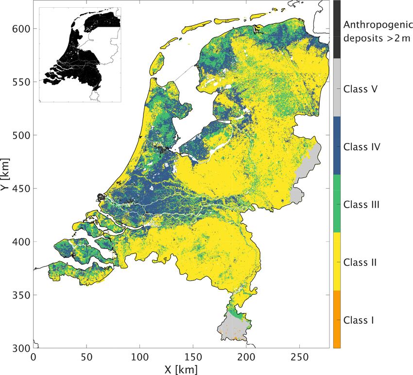
42                          J. van Ginkel et al.: Development of a seismic site-response zonation map for the Netherlands

face. This can be retrieved from in situ investigations; how-      of Pilz et al. (2009), Perron et al. (2018), and Panzera et al.
ever, this is a costly procedure. Because of the time and costs    (2021), who show a comparison of site-response techniques
involved, there is a lack of site-response investigations cover-   using earthquake data and ambient seismic noise analysis.
ing large areas, while the availability of detailed and uniform       The aim of this work is to design a site-response zonation
ground motion amplification maps is fundamental for prelim-        map for the Netherlands, which is both detailed and spatially
inary estimates of damage on buildings (e.g. Falcone et al.,       extensive. Rather than using ground motion prediction equa-
2021; Gallipoli et al., 2020; Bonnefoy-Claudet et al., 2009;       tions with generic site amplification factors conditioned on
Weatherill et al., 2020).                                          Vs30 , we propose a novel approach for the development of a
   Empirical seismic site response is widely investigated by       nationwide zonation of amplification factors. To this end, we
the use of microtremor horizontal-to-vertical spectral ratios      combine multiple seismological records, geophysical data,
(HVSRs; e.g. Fäh et al., 2001; Lachetl and Bard, 1994;             and detailed 3D lithostratigraphic models in order to esti-
Bonnefoy-Claudet et al., 2006a; Albarello and Lunedei,             mate and interpret site response. We first select the Gronin-
2013; Molnar et al., 2018; Lunedei and Malischewsky,               gen borehole network where detailed information on subsur-
2015). The HVSR is obtained by taking the ratio between the        face lithology, numerous earthquake ground motion record-
Fourier amplitude spectra of the horizontal and the vertical       ings, and ambient seismic noise recordings is available since
components of a seismic recording. When a shallow veloc-           their deployment in 2015. From this, we extract empirical
ity contrast is present, the peak in the HVSR curve is closely     relationships between seismic wave amplification and differ-
related to the shear-wave resonance frequency for that site.       ent lithostratigraphic conditions, building upon the proxies
However, the HVSR peak amplitude cannot be treated as the          defined in van Ginkel et al. (2019).
actual site amplification factor but rather serves as a qualita-      Next, the ambient vibration measurements of the seismic
tive estimate (Field and Jacob, 1995; Lachetl and Bard, 1994;      network across the Netherlands are used, necessary to cali-
Lermo and Chavez-Garcia, 1993).                                    brate the amplification (via HVSR) with the local lithostrati-
   The Netherlands experiences tectonically related seismic        graphic conditions. By combining the detailed 3D geological
activity in the southern part of the country, with magnitudes      subsurface models GeoTOP (Stafleu et al., 2011, 2021) and
up to 5.8 measured so far (Camelbeeck and Van Eck, 1994;           NL3D (van der Meulen et al., 2013), with a derived classi-
Houtgast and Van Balen, 2000; Paulssen et al., 1992). Addi-        fication scheme, a zonation map for the Netherlands is con-
tionally, gas extraction in the northern part of the Netherlands   structed.
regularly causes shallow (3 km), low-magnitude (Mw ≤ 3.6              The presented site-response zonation map for the Nether-
thus far) induced earthquakes (Dost et al., 2017). Over the        lands is especially designed for seismically quiet regions
last decades, an increasing number of these induced seismic        where tectonic seismicity is absent, but with a potential risk
events have stimulated the research on earthquake site re-         of induced seismicity, for example due to mining or geother-
sponse in the Netherlands. Various studies (van Ginkel et al.,     mal energy activity (Majer et al., 2007; Mena et al., 2013;
2019; Kruiver et al., 2017a, b; Bommer et al., 2017; Noor-         Mignan et al., 2015). As a result, this map can be imple-
landt et al., 2018) undertaken in the Groningen area (north-       mented in seismic hazard analysis.
eastern part of the Netherlands) concluded that the hetero-
geneous unconsolidated sediments are responsible for sig-
nificant amplification of seismic waves over a range of fre-       2   Geological setting and regional seismicity
quencies pertinent to engineering interest. Although the lo-
cal earthquake magnitudes are relatively small, the dam-           The Netherlands is positioned at the southeastern margin of
age to the houses can be significant. Hence multiple stud-         the Cenozoic North Sea basin. The onshore basin infill is
ies (e.g. Rodriguez-Marek et al., 2017; Bommer et al., 2017;       characterised by Paleogene, Neogene, and Quaternary sed-
Kruiver et al., 2017a; Noorlandt et al., 2018) were performed      iments reaching a maximum thickness of ∼ 1800 m. Mini-
on ground motion modelling including the site amplification        mum onshore thicknesses are reached along the basin flanks
factor for the Groningen region.                                   in the eastern and southern Netherlands and locally at up-
   Groningen forms an excellent study area due to the pres-        lifted blocks like the Peel Block. The main tectonic feature of
ence of the permanently operating borehole seismic network         the country is the Roer Valley Graben, bounded by the Peel
(G-network). Local earthquake recordings over the Gronin-          Boundary Fault in the northeast and the Rijen, Veldhoven,
gen borehole show that the largest amplification develops in       and Feldbiss faults in the south and southwest (Fig. 1).
the top 50 m of the sedimentary cover (van Ginkel et al.,             The Paleogene and Neogene sediments are dominated by
2019), although the entire sediment layer has a thickness of       marine clays and sands that were primarily deposited in shal-
around 800 m in this region. Furthermore, van Ginkel et al.        low marine environments. The Quaternary sediments, reach-
(2019) showed the existence of a correlation between the spa-      ing a maximum onshore thickness of ∼ 600 m, reflect a tran-
tial distribution of microtremor horizontal-to vertical spectral   sition from shallow marine to fluvio-deltaic and fluvial de-
ratio (HVSR) peak amplitudes and the measured earthquake           positional environments in the early Quaternary to a com-
amplification. This observation is in accordance with those        plex alternation of shallow marine, estuarine, and fluvial

Nat. Hazards Earth Syst. Sci., 22, 41–63, 2022                                       https://doi.org/10.5194/nhess-22-41-2022
J. van Ginkel et al.: Development of a seismic site-response zonation map for the Netherlands                                     43

Figure 1. Surface geological map of the Netherlands. Older deposits comprise unconsolidated Neogene and Paleogene deposits as well as
Mesozoic and Carboniferous limestones, sandstones, and shales. Modified after Schokker (2010). RF: Rijen Fault; VF: Veldhoven Fault;
PBF: Peel Boundary Fault; FBF: Feldbiss Fault; RVG: Roer Valley Graben.

sediments in the younger periods (Zagwijn, 1989; Rondeel             systems embedded in flood basin clays (Gouw and Erkens,
et al., 1996; De Gans, 2007; Busschers et al., 2007; Peeters         2007). The fluvial channel belts pass downstream into sandy
et al., 2016). Imprints of glacial conditions are recorded in        tidal channel systems in the coastal plain (Hijma et al., 2009).
the upper part of the basin fill by, among others, deep erosive         The Pleistocene interior of the country mainly consists of
structures (subglacial valleys, tongue basins) and glacial till      glacial, aeolian, and fluvial deposits (Rondeel et al., 1996;
(Van den Berg and Beets, 1987).                                      Van den Berg and Beets, 1987). Glacial deposits include
                                                                     coarsely grained meltwater sands and tills. Ice-pushed ridges,
2.1   Surface geology                                                with heights up to 100 m, occur in the middle and east of the
                                                                     country. Aeolian deposits mainly consist of cover sands and
The surface geology (Fig. 1) is mainly characterised by a            are locally made up by drift sand and inland dunes. In the
Holocene coastal barrier and coastal plain in the west and           south and east of the country, sandy channel and clayey flood
north and an interior zone with Pleistocene deposits cut by          basin deposits of small rivers occur.
a Holocene fluvial system (Rondeel et al., 1996; Beets and              Neogene and older deposits are only exposed in the
van der Spek, 2000). The coastal barrier consists of sandy           eastern- and southernmost areas of the country. In the east,
shoreface and dune deposits and is up to 10 km wide. It is in-       these sediments include unconsolidated Paleogene forma-
tersected in the south by the estuary of the Rhine, Meuse, and       tions as well as Mesozoic limestones, sandstones, and shales.
Scheldt and in the north by the tidal inlets of the Wadden Sea.      In the south, the older deposits comprise unconsolidated
The coastal plain is formed by mainly marine clay as well as         Neogene and Paleogene sands and clays, as well as Creta-
peat. Although much of the peat has disappeared because of           ceous limestones (chalk), sandstones and shales, and Car-
mining and drainage, thick sequences of peat (> 6 m) still           boniferous sandstones and shales.
occur. The Holocene fluvial deposits of the rivers Rhine and
Meuse are characterised by a complex of sandy channel belt

https://doi.org/10.5194/nhess-22-41-2022                                         Nat. Hazards Earth Syst. Sci., 22, 41–63, 2022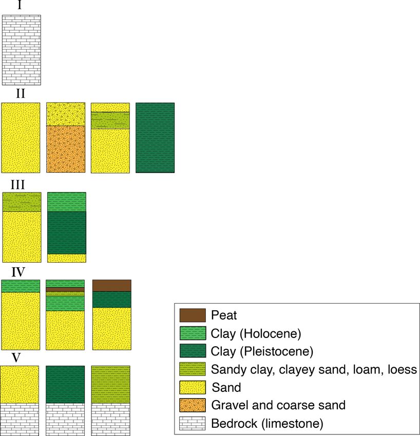
44                            J. van Ginkel et al.: Development of a seismic site-response zonation map for the Netherlands

Figure 2. Map of the Netherlands depicting epicentres of all induced (Mw 0.5–3.6, orange) and tectonic (Mw 0.5–5.8, yellow) earthquakes
from 1910–2020. The diameter of the circles indicates the relative earthquake magnitude. The triangles represent the surface location of the
borehole stations (blue), borehole stations with SCPT measurements (purple), and single surface seismometers (green). The triangles with
red outlines depict the locations of example HVSR curves presented in Fig. 8. The inset in the northeast depicts the location of the Groningen
borehole network (G-network). Here, the red triangle depicts the location of borehole G24. The 19 (Mw ≥ 2) induced earthquakes in this
panel are used for the AF and ETF computations. Coordinates are shown within the Dutch national triangulation grid (Rijksdriehoekstelsel
or RD), and lat–long coordinates are added in the corners for international referencing.

2.2   Regional seismicity                                                   Most induced earthquakes in the Netherlands (orange cir-
                                                                         cles, Fig. 2) have their epicentre in the Groningen region due
The Netherlands experiences tectonically related earthquake              to production of the gas field. Here, reservoir compaction due
activity in the southeast, and induced earthquakes occur in              to pressure depletion has reactivated the existing normal fault
the north at shallow depths due to exploitation of gas fields.           system that traverses the reservoir layer throughout the whole
Tectonic seismicity occurs mainly in the Roer Valley Graben              field. (Buijze et al., 2017; Bourne et al., 2014). Even though
(yellow circles, Fig. 2), which is part of a larger basin and            the magnitudes are relatively low (van Thienen-Visser and
range system in western Europe, the Rhine Graben Rift Sys-               Breunese, 2015), the damage to buildings in the area is sub-
tem. At the beginning of the Quaternary, the subsidence rate             stantial due to shallow hypocentres and amplification on the
in the Roer Valley Graben did increase significantly (Geluk              soft near-surface soils (Bommer et al., 2017; Kruiver et al.,
et al., 1995; Houtgast and Van Balen, 2000), and the rift                2017a).
system still shows active extension (Hinzen et al., 2020).
The largest earthquake recorded (Mw = 5.8) in the Nether-
lands was in Roermond in 1992, due to extensional activity               3    Dataset
along the Peel Boundary Fault (Paulssen et al., 1992). Gariel
et al. (1995) quantified the near-surface amplification based            For this study, we use the seismic network of the Royal
on spectral ratios of aftershocks from the 1992 earthquake               Netherlands Meteorological Institute (KNMI, 1993), consist-
in Roermond. They observed great variety in ground motion                ing of borehole and surface seismometers distributed over the
amplitudes over different stations, which is the site effect of          Netherlands (Fig. 2). The network includes 88 locations with
shallow sedimentary deposits.                                            vertical borehole arrays where each station is equipped with
                                                                         three-component 4.5 Hz seismometers at 50 m depth inter-
                                                                         vals (50, 100, 150, 200 m) and an accelerometer at the sur-

Nat. Hazards Earth Syst. Sci., 22, 41–63, 2022                                               https://doi.org/10.5194/nhess-22-41-2022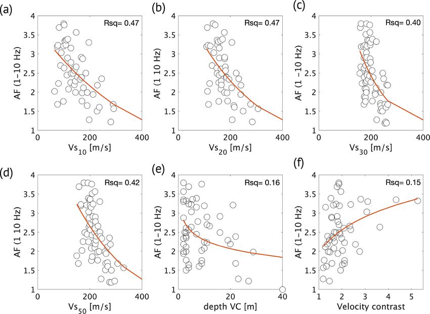
J. van Ginkel et al.: Development of a seismic site-response zonation map for the Netherlands                                   45

face. The southernmost station is at Terziet (TERZ). This         plification in order to evaluate which parameters are most
station consists of a borehole seismometer at 250 m depth         critical.
and a surface seismometer. In Groningen, multiple boreholes
have seismic cone penetration tests (SCPTs) taken directly        4.1   Definition of amplification
adjacent to the borehole. The remaining triangles represent
29 locations of single surface seismometers (accelerome-          The majority of site-response studies define the level of soft
ters and broad bands). All seismometers have three compo-         sediment amplification with respect to the surface seismic
nents and are continuously recording the ambient seismic          response of a nearby outcropping hard rock. In the Nether-
field and, when present, local earthquakes. In Sect. 4 we         lands, no representative seismic response of outcropping
use 19 local earthquakes of M ≥ 2, recorded in the Gronin-        bedrock is available. As an alternative, we define reference
gen borehole network between May 2015 and May 2019.               conditions as found in Groningen at 200 m depth, where
All data are available through the KNMI data portal (http:        we have many seismic recordings. These same reference
//rdsa.knmi.nl/network/NL/, last access: 1 June 2021).            conditions can be found at this depth over most locations
   In the construction of the site-response map, we have made     in the Netherlands, though it can sometimes be deeper or
extensive use of the detailed 3D geological subsurface mod-       shallower than 200 m. The corresponding elastic properties
els GeoTOP and NL3D. Both models are developed and                (shear-wave velocity and density) form the basis from which
maintained by TNO – Geological Survey of the Netherlands          the ground motion amplification effect of any site with re-
(van der Meulen et al., 2013). GeoTOP schematises the shal-       spect to the reference can be predicted. This approach is akin
low subsurface of the Netherlands in a regular grid of rect-      to the reference velocity profile that is used in Switzerland
angular blocks (voxels, tiles, or 3D grid cells), each mea-       (Poggi et al., 2011).
suring 100 m by 100 m by 0.5 m (x ,y, z) up to a depth               For a recording at the Earth’s surface, the upward and
of 50 m below ordnance datum (Stafleu et al., 2011, 2021).        downward waves are simultaneously recorded, which leads
Each voxel contains multiple properties that describe the ge-     to an amplitude doubling. This is called the free-surface ef-
ometry of lithostratigraphic units (formations, members, and      fect. If the amplification is defined with respect to a surface
beds), the spatial variation in lithology, and sand grain size    (hard-rock) site, both the site of investigation and the refer-
within these units as well as measures of model uncertainty.      ence site experience the same free-surface effect, and there is
GeoTOP is publicly available from the TNO’s web portal:           no need to remove it in order to isolate the relative amplifica-
https://www.dinoloket.nl/en/subsurface-models (last access:       tion. We have a reference site at depth, where no free-surface
1 August 2021). To date, the GeoTOP model covers about            effect takes place. Hence, we need to remove the free-surface
70 % of the country (including inland waters such as the          effect first from the surface recording before isolating the rel-
Wadden Sea). For the missing areas we have used the lower-        ative amplification.
resolution voxel model NL3D, which is available for the en-          The G-network forms a representative resource for the def-
tire country (van der Meulen et al., 2013). NL3D models           inition of the reference horizon parameters. Hofman et al.
lithology and sand grain-size classes within the geological       (2017) and Kruiver et al. (2017a) determined shear-wave
units of the layer-based subsurface model DGM (Gunnink            velocities at all borehole seismometer levels in Gronin-
et al., 2013) in voxels measuring 250 m by 250 m by 1 m (x,       gen. From their velocities found at 200 m depth, the aver-
y, z) up to a depth of 50 m below ordnance datum. To deter-       age is taken, resulting in a reference shear-wave velocity
mine the depth of bedrock in the shallow subsurface, we con-      of 500 m/s. At this depth, the sediment density is on av-
sulted the layer-based subsurface models DGM and DGM-             erage 2.0 kg/m3 . At 200 m depth, 95 % of the Dutch sub-
deep. These models are also available from the web portal         surface is composed of laterally extensive Pleistocene and
mentioned above. More details on the models GeoTOP and            Pliocene sediments; hence the estimated site-response and
NL3D are given in Appendix B.                                     corresponding amplification factors can be applied to a large
                                                                  part of the country. The remaining 5 % consists of shallow
                                                                  (< 100 m) Triassic, Cretaceous, and locally Carboniferous
                                                                  bedrock, and therefore these locations need to be evaluated
4   Empirical relationships from the Groningen borehole           separately.
    network
                                                                  Frequency bandwidth
The dense Groningen borehole network (G-network) pro-
vides the opportunity to derive empirical relationships be-       Data processing is applied to a frequency band-pass filter
tween measured amplification in the time and frequency do-        for 1–10 Hz, covering the periods of interest from an earth-
main, estimated amplification from ambient vibrations, and        quake engineering point of view. Moreover, for these fre-
the local lithostratigraphic conditions. First, we present re-    quencies, the used instrumentation (broadband seismome-
sults of three different methods to assess amplification. Next,   ters, accelerometers, and geophones) has high sensitivity for
we compare subsurface parameters with the measured am-            ground motion.

https://doi.org/10.5194/nhess-22-41-2022                                      Nat. Hazards Earth Syst. Sci., 22, 41–63, 2022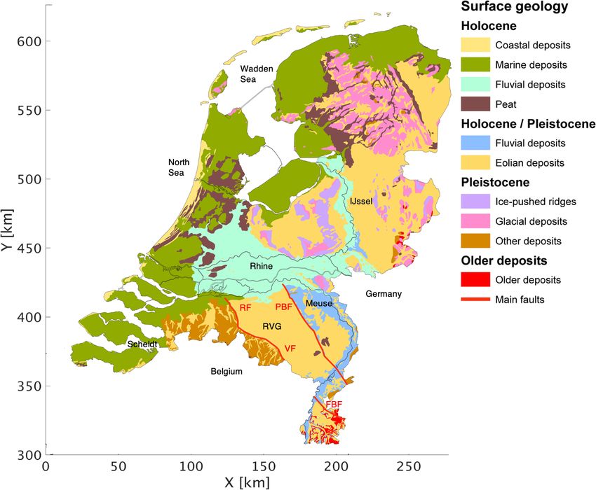
46 J. van Ginkel et al.: Development of a seismic site-response zonation map for the Netherlands
Figure 3. (a) Particle velocity Fourier amplitude spectrum measured on the radial component for the 200 m (grey) and surface seismometer
(blue) for borehole G24 for a 20 s time window of the 8 January 2018 Zeerijp M 3.4 earthquake. Borehole G24 has an epicentral distance of
10 km. (b) Shear-wave velocity profile for G24 with the interval velocities from Hofman et al. (2017) in blue and the shear-wave velocity from
the adjacent SCPT over the top 30 m (black line). The corresponding lithological profile is derived from GeoTOP (https://www.dinoloket.nl/
en/subsurface-models, last access: 15 October 2021).
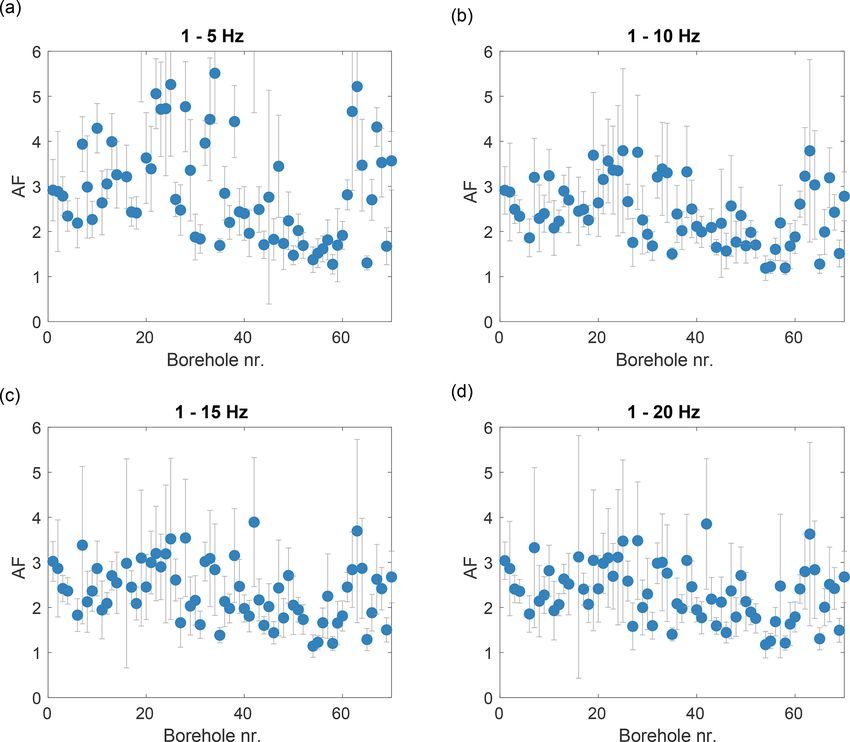
Since most of the amplification is occurring in the top sed- choice for the specific AF frequency band was supported
imentary layer (van Ginkel et al., 2019), the corresponding by evaluating amplification over a range of frequency bands.
resonance frequencies are covered in the used frequency fil- Figure 4 shows the AFs over the Groningen network for sev-
ter as well. Above 10 Hz, the amplitude increase due to soil eral bands. AF values are highest in the band 1–5 Hz due
softening and resonance is counteracted by an elastic attenu- to the strong resonances of the Holocene infill (van Ginkel
ation and 3D scattering. Furthermore, what exactly happens et al., 2019). In the 1–10 Hz band the AFs are lower but con-
above 10 Hz is of little interest since most of the local earth- tain considerable earthquake amplitudes (Fig. 3). When the
quake energy is contained in the frequency band between 1 frequency band is extended beyond 10 Hz (Fig. 4c and d), the
and 10 Hz. This is illustrated in Fig. 3, which presents the AF values do not change significantly. We decided to pick the
particle velocity Fourier amplitude spectrum of a local earth- frequency band of 1–10 Hz as the representative AF since
quake recorded in borehole G24. The location of this bore- it is a better overall representation of amplification by the
hole is presented as a red triangle in Fig. 2. soft sediments than the higher values of 1–5 Hz, as shown in
Wassing et al. (2012).
4.2 Amplification factors
4.3 Empirical transfer functions
We compute an overall amplification factor from the G-
network earthquake recordings by taking the ratio of the
maximum amplitudes recorded at the surface and the 200 m Empirical transfer functions (ETFs) represent shear-wave
deep seismometer, following the procedure described in van amplification in the frequency domain. ETFs are defined as
Ginkel et al. (2019). This ratio is taken for both the radial a division of the Fourier amplitude spectra at two different
(R) and transverse (T ) components, and the results are av- depth levels. With a reference horizon at 200 m depth and
eraged. The amplitude at the surface is divided by a factor the level of interest at the Earth’s surface, the transfer func-
of 2 in order to remove the effect of the upward and down- tion has both a causal and acausal part. The causal part maps
ward waves recorded at the same time. Earthquake records upward-propagating waves, from the reference level to the
are processed in the time domain for a 20 s time window and surface. The acausal part maps downward-propagating waves
frequency band of 1–10 Hz. Next, the AF for each borehole back to the free surface (Nakata et al., 2013). When describ-
is obtained by repeating the above procedure for 19 available ing amplification, we are only interested in the causal part.
M ≥ 2.0 local induced earthquakes and subsequently aver- We select this causal part of the estimated transfer function
aging the values. It is determined in the time domain and and compute its Fourier amplitude spectrum to obtain a mea-
therewith provides an average amplification over the applied sure of frequency-dependent amplification. We use 20 s long
frequency band. time windows for particle velocity recordings on the radial
Many studies (e.g. Bommer et al., 2017; Rodriguez-Marek component of the G-network seismometers. Subsequently,
et al., 2017; Borcherdt, 1994) model site-response amplifica- we average over 19 local earthquakes with magnitudes ≥ 2.0.
tion factors (AFs) for different periods of spectral accelera- This can be seen as an implementation of seismic interfer-
tions, which tailors to engineering structures with different ometry by deconvolution (Wapenaar et al., 2010). Lastly, the
resonance frequencies. In this study we aim to provide an deconvolution results are stacked to enhance stationary con-
average amplification level in a broad frequency band. The tributions.
Nat. Hazards Earth Syst. Sci., 22, 41–63, 2022 https://doi.org/10.5194/nhess-22-41-2022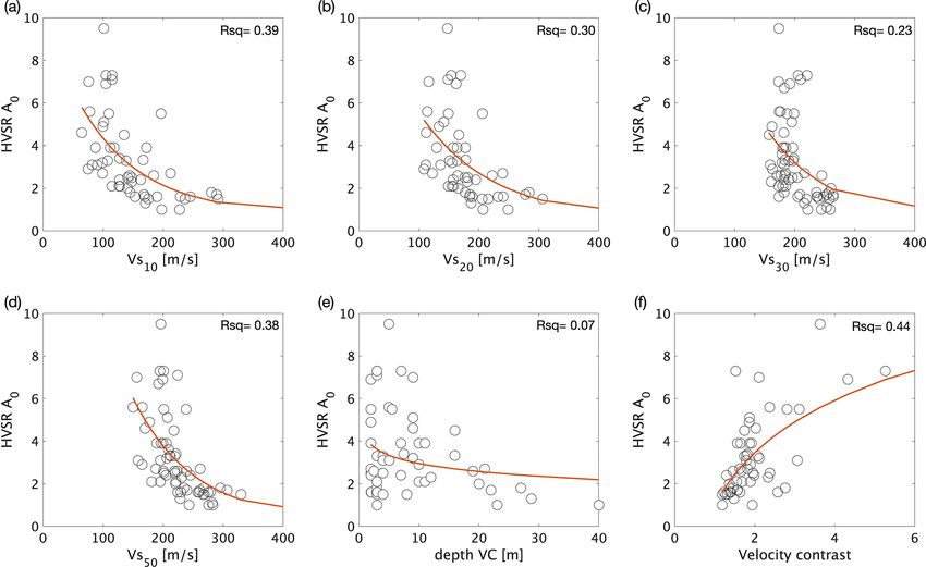
J. van Ginkel et al.: Development of a seismic site-response zonation map for the Netherlands                                                 47

Figure 4. Amplification factors (AFs) for (a) frequency bands 1–5 Hz, (b) 1–10 Hz, (c) 1–15 Hz, and (d) 1–20 Hz and corresponding standard
deviations (error bars) associated with the averaged AFs over 19 M ≥ 2.0 local earthquakes.

Figure 5. Probability density function of 1 month of daily HVSRs and the mean HVSR (solid black line) and ETF for the borehole seismome-
ter interval of 0–50 m (grey dashed line) and 0–200 m (grey solid line). The selected borehole sites exhibit differences in curve characteristics
with (a) G24 illustrating clearly peaked curves (> 4), (b) G16 illustrating medium (2–4) peak amplitudes, and (c) G51 with no pronounced
peak.

   From the ETF between the 200 m depth and surface seis-                  peak amplitudes are measured at sites with unconsolidated
mometer (ETF200 ), peak amplitudes are identified. Some ex-                Holocene alternations of clay and peat, overlying consoli-
ample ETF curves are plotted in Fig. 5. Additionally, ETF                  dated Pleistocene sediments.
curves for the top 50 m are calculated (ETF50 ). The ETF
curves for the different intervals show very similar peak char-            4.4   H /V spectral ratios from the ambient seismic field
acteristics and peak amplitudes, demonstrating that most am-
plifications are developed in the top 50 m of the sediment                 The Groningen surface seismometers are continuously
cover. Furthermore, the borehole sites with the highest ETF                recording the ambient seismic field (ASF), and these data
peak amplitudes can be linked to the local geology, as pre-                are used to estimate horizontal-to-vertical spectral ratios
sented in van Ginkel et al. (2019, Fig. 9). Here, highest                  (HVSR). In this study we focus on the second peak (≥ 1 Hz)

https://doi.org/10.5194/nhess-22-41-2022                                                Nat. Hazards Earth Syst. Sci., 22, 41–63, 2022
48                             J. van Ginkel et al.: Development of a seismic site-response zonation map for the Netherlands

                                                                         4.5   Amplification parameters

                                                                         Across the Netherlands, the ASF is continuously recorded on
                                                                         all seismometers, while many locations lack recordings of lo-
                                                                         cal earthquakes. Therefore we further investigate whether the
                                                                         HVSR can be used as a proxy for amplification as measured
                                                                         by the earthquake-derived ETF and AF. Figure 6 displays
                                                                         the correlation between the peak amplitudes of the HVSR
                                                                         and ETF200 as well as HVSR and AF. Secondly, we evaluate
                                                                         the subsurface seismic parameters enhancing amplification
                                                                         (Fig. 7).
                                                                            Based on these data points, relationships are defined in or-
                                                                         der to be able to estimate amplification factors using HVSR
                                                                         peak amplitudes (A0 ), amplification factors:
                                                                         AF = 1.49 + 0.87 log(1.12A0 ),                              (1)
Figure 6. Relation between the HVSR peak amplitudes (A0 ) and            and maximum amplification as measured by the ETF:
the ETF peak amplitudes (grey) and the HVSR peak amplitudes and
the AF (blue). The solid line represents the fitting function (Eqs. 1    ETF = 1.08 + 6.89 log(1.09A0 ).                             (2)
and 2) between the HVSR peak amplitudes and the measured ampli-          The relationship between the AF derived from the Groningen
fication from AF and ETF, respectively. Rsq (R-squared) represents
                                                                         borehole locations and local site conditions is investigated in
the coefficient of determination of the fitting. Note the log-scale of
the y axis.
                                                                         the following.
                                                                            Many ground motion prediction equations which include
                                                                         site response consider the shear-wave velocity for the top
                                                                         30 m (Vs30 ) as the main parameter affecting amplification
in the HVSR curve, which represents shear-wave resonances                (Akkar et al., 2014; Bindi et al., 2014; Kruiver et al., 2017b;
at the shallowest interface of soft sediments on top of more             Wills et al., 2000), as well as Eurocode 8 (Comité Européen
consolidated sediments. Resonances of the complete sedi-                 de Normalisation, 2004). However, studies (Castellaro et al.,
ment layer display a peak at lower frequencies (van Ginkel               2008; Kokusho and Sato, 2008; Lee and Trifunac, 2010) have
et al., 2020). Above 1 Hz the noise field is dominated by                drawn attention to the fact that using only Vs30 as a proxy
anthropogenic sources. The details of the method to obtain               for site response is inadequate, because it does not uniquely
stable HVSR curves from the ASF in the Groningen bore-                   correlate with amplification. They show that amplification is
hole network can be found in van Ginkel et al. (2020). In                defined by several parameters, including the depth and de-
summary, from power spectral densities for each component,               gree of the seismic impedance contrast. Furthermore Joyner
the H /V division is performed for each day. Subsequently,               and Boore (1981) introduce the shear-wave velocity ratio be-
a probability density function is computed over one month                tween the top and base layers as a proxy for site amplifica-
of H /V ratios and the mean is extracted. This yields a sta-             tion, and this is further explored by Boore (2003).
ble HVSR curve that is not much affected by transients like                 In order to assess the impact of different parameters,
nearby footsteps or traffic.                                             firstly, the AF at each borehole location is fitted against sev-
   Based on the HVSR curve and peak characteristics, dif-                eral subsurface parameters. AF = a + b · ec·Vs as a functional
ferent criteria are defined conformable to the SESAME con-               form, where a, b, and c are unknown coefficients to be fitted.
sensus (Bard, 2002): (1) clear peaked curves (HVSR ampli-                This fitting is applied with averaged shear-wave velocities
tude > 4) related to a sharp velocity contrast in the shallow            over various depth intervals. Vs10 , Vs20 , and Vs30 -values are
subsurface. (2) HVSR peak amplitude between 2–4, associ-                 derived from SCPTs, acquired directly adjacent to 53 bore-
ated with a weak velocity contrast. (3) No distinguishable               hole sites in Groningen (Fig. 2). Hofman et al. (2017) de-
peak and a flat curve indicate the absence of a velocity con-            rived interval velocities determined from the G-network, us-
trast in the shallow subsurface. Example HVSRs for these                 ing seismic interferometry applied to local induced events.
three criteria are plotted in Fig. 5. Its associated peak ampli-         The velocities from this reference are used to determine
tudes are derived from the mean HVSR curve and presented                 Vs50 . Secondly, from the SCPT data we derive the depth
in van Ginkel et al. (2019). The correlation between peaks               and size of the velocity contrast. The contrast is computed
on the HVSR curves and the presence of a velocity contrast               by the division of the two different velocity values bounding
at some depth is stressed in studies from Bonnefoy-Claudet               each 1 m interval. This division is done for each 1 m interval
et al. (2008), Konno and Ohmachi (1998) and Lermo and                    over the 30 m of SCPT records. The largest division value
Chavez-Garcia (1993) and this contrast is very likely to am-             is defined as the (main) velocity contrast (VC), and corre-
plify the ground motion.                                                 sponding depth is the depth of the contrast (zVC). Thereafter

Nat. Hazards Earth Syst. Sci., 22, 41–63, 2022                                             https://doi.org/10.5194/nhess-22-41-2022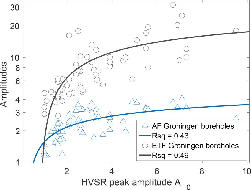
J. van Ginkel et al.: Development of a seismic site-response zonation map for the Netherlands 49
Figure 7. Each panel depicts the fitted function and the coefficient of determination (Rsq ) of the AF (1–10 Hz) per G-network borehole
location and the corresponding subsurface parameter. (a) Vs10 , (b) Vs20 , (c) Vs30 , (d) Vs50 , (e) depth of the velocity contrast, and (f) size of
the velocity contrast.
the VC values and their depth are fitted with the AF using for amplification. Therefore, for all surface seismometers in
AF = a + b · log(c · VC) as a functional form. This procedure the Netherlands seismic network, the HVSR curves are es-
is also performed for the relation between the subsurface pa- timated following the method described in Sect. 4.4. Fig-
rameters (Vs , VC) and the HVSR. The results are given in ure 8 displays a selection of representative examples of
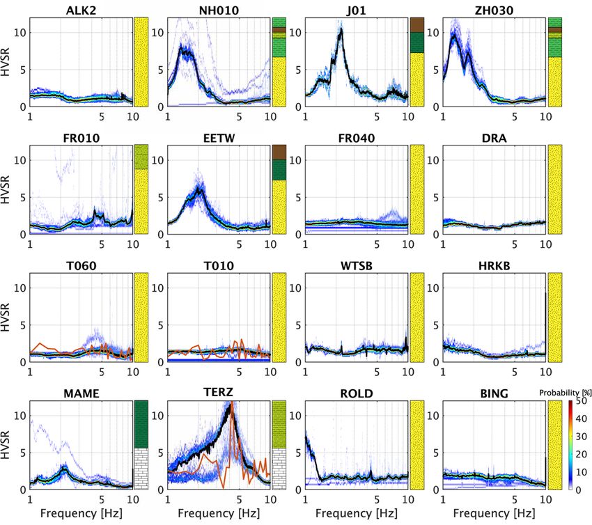
Appendix A. HVSR curves. It also includes the sediment classification
Figure 7 presents the fit between the AF and the six rele- profile presented in Sect. 6 and Fig. 9. In addition, for bore-
vant subsurface parameters. Best fit (Rsq = 0.47, Fig. 7a and holes T010, T060, and TERZ, the ETF curve is added, cal-
b) is observed between the AF and Vs10 and Vs20 . This is in culated from local earthquakes similar to the approach de-
line with findings of Gallipoli and Mucciarelli (2009), who scribed in Sect. 4.3. These 16 HVSR curves illustrate the di-
use the Vs10 as the main amplification parameter instead of versity in curve characteristics throughout the Netherlands.
the more common Vs30 . In Groningen, the low-velocity and Here, we can distinguish the three types of curves as de-
unconsolidated Holocene sediments have a thickness of 1 to scribed in Sect. 4.4. The flat curves with no distinguishable
25 m, and below these depths the velocities increase in the peak (FR040, DRA, T060, T010, WTSB, HRKB, ROLD,
more compacted Pleistocene sediments. The reduced fitting and BING) are recorded at seismometers on top of outcrop-
quality of Vs30 and Vs50 arises since the amplification de- ping Pleistocene sands (Holocene–Pleistocene aeolian and
velops mainly in the Holocene sediments (van Ginkel et al., fluvial deposits in Fig. 1). Also, ALK2 exhibits no peak am-
2019). Although the fit is relatively poor, a relationship is plitude since this seismometer is positioned on dune sands
observable between a large VC and an elevated AF (Fig. 7e). (Holocene coastal deposits in Fig. 1). These locations are
By contrast, Fig. A1 presents a good correlation between VC characterised by absence of a strong velocity contrast in the
and HVSR. A large VC value leads to resonance in the near shallow subsurface. Selected examples of HVSR curves ex-
surface, which is expressed in high-amplitude peaks of the hibiting clear peak amplitudes (NH01,J01, ZH030, FR010,
HVSR. EETW) are located at sites with a distinct velocity contrast
between unconsolidated Holocene marine sediments overly-
ing Pleistocene sediments.
5 HVSR estimations throughout the Netherlands In the southernmost part of the Netherlands, Cretaceous
bedrock is either outcropping or situated less than 100 m
Based on the good relationship between Groningen HVSR
deep. MAME and TERZ are examples of locations with soft
peak amplitudes (A0 ), ETF peak amplitudes, and AF (Fig. 6),
we conclude that the HVSR can be further used as proxy
https://doi.org/10.5194/nhess-22-41-2022 Nat. Hazards Earth Syst. Sci., 22, 41–63, 2022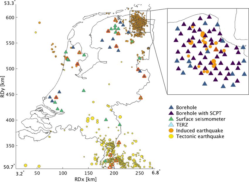
50                           J. van Ginkel et al.: Development of a seismic site-response zonation map for the Netherlands

Figure 8. Each panel depicts a probability density function from ambient noise HVSR curves and sediment classification profile (Sect. 6) for
16 stations of the NL network. The black line represents the mean HVSR, and the red line in the panels of T06, T010, and TERZ represents
the ETF calculated from 10 local earthquakes. The colour bar in the lower right displays the HVSR probability range that is valid for all
panels.

sediments overlying hard rock, and the HVSR curves exhibit              cells are populated with a site-response class with a corre-
a clear peak amplitude.                                                 sponding AF.

                                                                        6.1    Classification scheme
6    Zonation map for the Netherlands
                                                                        The borehole ETFs confirm that most of the amplification is
The effect of local site response on earthquake ground mo-              developed in the top 50 m (Fig. 5) of the sedimentary cover,
tion is included in the Eurocode 8 seismic design of buildings          corresponding to the findings in van Ginkel et al. (2019). Be-
(Comité Européen de Normalisation, 2004, EC8). In order                 yond 50 m depth, the Quaternary deposits mainly consist of
to estimate the risk of enhanced site response, EC8 presents            more compacted marine and fluvial sediments. Therefore the
five soil types based on shear-wave velocities and strati-              sediment classification presented in this section uses the top
graphic profiles. Soil type E is essentially characterised by           50 m with a special focus on the top 10 m. Also, the pres-
a sharp contrast of a soft layer overlying a stiffer one. How-          ence of a velocity contrast is used in the classification, as it
ever, in our opinion, this single classification for soft sedi-         was shown to have a (albeit weaker) link with amplification
ments is rather limited, especially concerning the wide va-             (Figs. 7 and A1).
riety of lithostratigraphic conditions throughout the Nether-              Following Convertito et al. (2010) and from the studies by
lands. Therefore, we present an alternative, or extended, clas-         Kruiver et al. (2017a) and van Ginkel et al. (2019), the Eu-
sification for ground characteristics designed to specify the           rocode 8 classification requires modification, caused by the
large heterogeneity in site conditions than exists within Eu-           heterogeneous shallow sediment composition and bedrock
rocode 8 ground type E.                                                 depth of the Dutch subsurface. Table 1 lists the criteria for the
   In this section, in a few steps, the site-response zonation          classification division defined for the Netherlands (NL clas-
map for the Netherlands is derived. For this, the country is            sification). The NL classification is divided into five classes
subdivided into grid cells. As a result, about 95 % of the grid         based on the top 50 m lithostratigraphic composition, the ve-

Nat. Hazards Earth Syst. Sci., 22, 41–63, 2022                                              https://doi.org/10.5194/nhess-22-41-2022
J. van Ginkel et al.: Development of a seismic site-response zonation map for the Netherlands 51
Table 1. Details of the NL classification. The Vs10 and velocity contrast (VC) values assigned to each class are based on the amplification
relationships presented in Sect. 4 and Appendix A. For class V there are no empirical data available relating Vs10 and VC with A0 (HVSR
peak amplitude), hence not determined (n.d).
Class Description top 200 m Vs10 [m/s] VC A0
I Hard rock > 800 – –
II Stiff sediment > 200 none or < 1.5 2.0 >4
V soft sediment on hard rock (< 100 m) no data no data n.d.
locity contrast (VC), and average shear-wave velocity for the
top 10 m.
For setting up the classification, we initially use A0 , the
peak amplitude from HVSR. We only have measured AF in
Groningen, whereas we have measured A0 for many sites
throughout the Netherlands (all stations depicted in Fig. 2).
Moreover, we found a clear relationship between A0 and AF
(Eq. 1). The relationships between Vs10 , VC, and A0 are esti-
mated from lithological conditions in Groningen, where the
sites are assigned to Classes II, III, and IV. For Classes I and
V we have insufficient empirical constraint on A0 and AF.
Only sites with bedrock at depths shallower than 100 m fall
into Class V, for which the resonance over the complete un-
consolidated cover can reach frequencies larger than 1 Hz.
Therewith, these sites become distinct from Classes II, III,
and IV, where such resonances occur at frequencies < 1 Hz.
At these lower frequencies, there is no match with resonance
periods of most building types in the Netherlands.
The short lithological description in Table 1 is not suffi-
cient to classify each site. To further aid the classification,
representative sediment profiles are obtained (Fig. 9) based
on the lithologic class sequences of the GeoTOP and NL3D.
Figure 9. Sediment profiles corresponding to the classification pre-
By grouping the main sediment profiles into the classes, we sented in Table 1, where the different columns are typical examples
link the lithostratigraphic conditions to the expected ampli- of the top 50 m of the Netherlands. The division in classes is based
fication behaviour of the shallow subsurface. The classifica- on the shallow subsurface composition related to the expected level
tion is tested and optimised using all the sites with an esti- of wave amplification during a seismic event.
mated HVSR curve. The next step is to attribute a class to
each lithostratigraphic profile per grid cell in the GeoTOP
and NL3D models. on each of the processing steps are given in Appendix C. The
next step is to attribute an amplification factor to each class.
6.2 Lithology-based classification
6.3 Amplification factors for the Netherlands
Based on the site-response amplification estimated with the For shake-map implementations or seismic hazard analysis,
HVSR peak amplitudes at 115 sites, we have categorised amplification factors (AFs) are usually derived from the Vs30
each sedimentary profile (Fig. 9) into a class. The next step is (e.g. Borcherdt, 1994). In this study, we estimate AFs by
to substitute GeoTOP and NL3D into these five classes. This substituting the HVSR peak amplitudes (A0 ) for 115 sta-
geologically based method allows the determination of site tions throughout the Netherlands into Eq. (1). This allows
response on regional and nationwide scales. Figure 10 gives the calculation of nationwide applicable AF values (AFNL )
a general outline of the procedure used to assign the appro- assigned to each of the classes presented in Fig. 9.
priate sediment class to each of the voxel stacks in GeoTOP In order to obtain an AFNL for each class, the 115 cal-
and NL3D. A voxel stack is the vertical sequence of voxels culated AFs are plotted against their site sediment class in
at a particular (x, y) location in GeoTOP or NL3D. Details Fig. 11a. For these 115 locations, the sediment classes are
https://doi.org/10.5194/nhess-22-41-2022 Nat. Hazards Earth Syst. Sci., 22, 41–63, 202252 J. van Ginkel et al.: Development of a seismic site-response zonation map for the Netherlands Figure 10. General outline of the vertical voxel-stack analysis used to assign the appropriate sediment class into each grid cell of the GeoTOP and NL3D geological models in the construction of the site-response zonation map. manually assigned based on the geological models, SCPT, or the farthest south and east of the Netherlands, so these areas other geological data available. From the AF distributions, fall into Classes I and V. There are too few data to calibrate the mean AF values (AFNL ) and corresponding standard de- the corresponding amplification factor. viation (σAF ) are calculated for each class (Table 2). In Class By applying the workflow that we introduced in Sect. 6.2, II there are a number of sites with exactly the same AF of automatic classification for the 115 sites is performed based 1.6. These are sites with no distinguishable peak, where A0 on GeoTOP and NL3D and plotted against the AF (Fig. 11b is set to 1, which yields, after filling out in Eq. (1), AF = 1.6. and c). Due to uncertainties in the models (Appendix C), The AFNL values are valid on a national scale for a fre- these distributions deviate from the manual classification quency range of 1–10 Hz and for reference conditions of (Fig. 11a). Note that for the manual classification SCPT in- Vs = 500 m/s (Sect. 4.1). There are no AF values for sites in formation could be used at 53 sites for which local infor- Nat. Hazards Earth Syst. Sci., 22, 41–63, 2022 https://doi.org/10.5194/nhess-22-41-2022
J. van Ginkel et al.: Development of a seismic site-response zonation map for the Netherlands 53
Figure 11. Comparison of calculated AF distribution in terms of manual classification (a) and automatic classification by GeoTOP (b) and
by NL3D (c). The locations where the empirical AF relationship is not valid are eliminated (Classes I and V). The red central mark indicates
the median; the bottom and top edges of the box indicate the 25th and 75th percentiles, respectively. The whiskers extend to the most extreme
data points, and the outliers (1.5× away from the interquartile range) are plotted individually as red circles.
mation is not included in GeoTOP and NL3D. We therefore Table 2. Amplification factors and standard deviations (σ ) for the
distinguish two types of uncertainty. NL classification. σAF is the uncertainty when a local (HVSR)
recording is available. σ GeoTOP and σ NL3D represent the addi-
1. σAF . This is the variability that originates from the clas- tional uncertainty associated with the GeoTOP and NL3D models.
sification. Within the classification, a number of differ-
ent sites are binned into the same class (Fig. 9), although Class AFNL σAF σ GeoTOP σ NL3D
in reality there is still a range of amplification behaviour. II 1.94 0.30 – –
This variability is approximated with the outcome of the III 2.4 0.28 0.32 0.34
manual classification (Fig. 11a), which could be done in IV 3.03 0.34 – –
great detail.
2. σmod . The geological models are geostatistical models
where not all grid cells contain individual lithological
data. Hence, there is an uncertainty of the actual litho- Some areas show a large scatter in classes, which is de-
logical succession at each grid cell. The total uncer- rived from a large heterogeneity in the near surface as rep-
tainty q
σtot (derived from Fig. 11b and c) can be writ- resented in the lithostratigraphic models. Typically, at these
ten as σAF 2 + σ 2 . By additionally averaging over the places there is large model uncertainty, for example in north-
mod
east North Holland (Fig. 13a). Here, the Holocene lithologi-
classes (labelled with subscript i ), we find the model
cal successions are very heterogeneous in terms of clay, peat,
uncertainty σmod :
and clayish sand. This region also exhibits discrepancies be-
n q tween the model’s lithological successions and HVSR curve
1X
σmod = σtot,i 2 − σAF,i 2 . (3) characteristics, for instance with seismometers J01 (Fig. 8)
n i=1 and J02. The geological model at these locations presents
large portions of clayish sand, resulting in Class III, while
Table 2 lists the mean AF values, the uncertainty in AF (σAF ), the HVSR curves exhibit distinctive, high-amplitude peaks,
and the uncertainty (σ ) for the GeoTOP and NL3D models. demonstrating local conditions related to Class IV.
For larger sedimentary bodies, like the dune area, there is
6.4 Site-response zonation map less model uncertainty. Dune sand is identified as Class II,
and here, the HVSR of the seismometers (e.g. ALK2, Fig. 8)
The workflow presented in Fig. 10 results in a class category lacks any peak due to the absence of a velocity contrast in the
assigned to each grid cell of the GeoTOP and NL3D models. near surface.
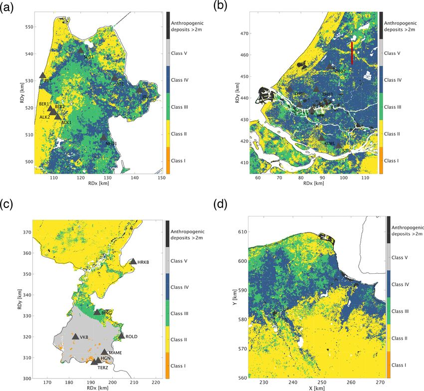
As a result, we present the national site-response zonation Figure 13b covers the “Randstad” region, the most densely
map (Fig. 12), where each class characterises a certain level urbanised part of the Netherlands, where the class is mainly
of expected site-response amplification. Additionally, each determined as IV. Figure 13c shows the southeastern part.
class has an AFNL assigned (Table 1). Figure 13 presents four Most of the northern part of this region is Class II due to
zoom-in panels of the map, each depicting a region of partic- Pleistocene sands reaching the surface. Most of the southern
ular interest. part of this region falls into Class V since the bedrock oc-
https://doi.org/10.5194/nhess-22-41-2022 Nat. Hazards Earth Syst. Sci., 22, 41–63, 202254 J. van Ginkel et al.: Development of a seismic site-response zonation map for the Netherlands
Figure 12. Seismic site-response zonation map for the Netherlands designed for low-magnitude induced earthquakes. The GeoTOP model
coverage is highlighted in black in the small inset. For the remaining part of the Netherlands, the NL3D model is used as the foundation for
the classification. The white spots are water bodies. The amplification factors and related uncertainties are presented in Table 2.
curs at a depth less than 100 m. A few places with bedrock because it may seriously affect the amplitude of the HVSR as
outcrops fall into Class I. shown in Guillier et al. (2007) and Molnar et al. (2018). We
Since Groningen has been studied in much detail, we also resolved this problem by using large portions (30 d) of noise
present the site-response zonation for this region (Fig. 13d) data to create stable HVSR curves (van Ginkel et al., 2020).
and discuss this in Sect. 7. It is important to mention the qualitative character of the mi-
crotremor HVSR peak amplitudes, which in themselves do
not directly relate to the amplification of a signal at the sur-
7 Discussion face during an earthquake. However, the microtremor HVSR
curve characteristics show major similarities with the mea-
The seismic site-response zonation map presented in Fig. 12
sured amplification from earthquake ETFs (Fig. 5), but not
distinguishes five classes, each of which defines the poten-
in terms of absolute values. Therefore an additional fitting
tial of occurrence of the related site-response amplification.
relationship (Eq. 1) has been defined, suitable for use of the
Here, the lithological conditions are collated into zonations
microtremor HVSR peak amplitudes as proxies for amplifi-
(classes) using the classification as shown in Fig. 9. In the de-
cation. HVSR measurements have proven to be very infor-
velopment of the lithostratigraphically based classification,
mative for site-response estimation and remain a valuable in-
we used (i) HVSR peak amplitudes, (ii) the presence of a
put for seismic site-response zonation (Molnar et al., 2018;
velocity contrast at depth, (iii) shear-wave velocities. Ampli-
Bonnefoy-Claudet et al., 2009).
fication factors are assigned to each class. In the following
Considering the difficulty in observing sufficient numbers
paragraphs we discuss the validity and uncertainties of the
of earthquake ground motions in areas that are not seismi-
classification, the AF distributions, and the usage and limita-
cally active, or where no large seismic networks are avail-
tions of the presented map.
able, we resorted to deriving and calibrating a lithology-
Since the ambient noise sources in the frequency band of
based classification scheme. We took advantage of the de-
interest (1–10 Hz) partly have an anthropogenic origin, one
tailed models of Cenozoic lithostratigraphy which are avail-
should be careful about contamination by local strong noise
Nat. Hazards Earth Syst. Sci., 22, 41–63, 2022 https://doi.org/10.5194/nhess-22-41-2022J. van Ginkel et al.: Development of a seismic site-response zonation map for the Netherlands 55
Figure 13. Panels highlighting different regions in the site-response zonation map, including the seismometer locations. (a) North Holland:
with a heterogeneous pattern between Classes III and IV. (b) The densely urbanised area of South Holland: the red line indicates the S–N
cross section through the GeoTOP voxel model (Fig. C1). (c) Limburg is in the north, a quite homogeneous zone of Class II, while the south
is dominated by Classes I and V due to shallow and outcropping bedrock. (d) Northeast Groningen is added as a comparison to other studies
performed in that region. No seismometer locations are plotted here because of the high density covering the map.
able in the Netherlands. As a consequence, the site-response cone penetration test (SCPT) to get a local shear-wave veloc-
map (Fig. 12) exhibits a regional pattern which is rather sim- ity profile.
ilar to the geological map (Fig. 1). We showed that the use of Rodriguez-Marek et al. (2017) defined a site-response
these models yields additional uncertainty in the determina- model including magnitude- and distance-dependent lin-
tion of the AF (Table 2). This uncertainty of the actual lithos- ear amplification factors (AFGr ) for several period intervals
tratigraphic profile at a site can be circumvented by a local (0.01–1.0 s) for the Groningen region as input for ground
recording. This may be an HVSR to obtain more certainty motion prediction equations by Bommer et al. (2017). This
on the site effect (Table 1), a cone penetration test (CPT) to site-response model starts from a reference horizon at the in-
obtain constraints on the lithology, or, better still, a seismic terface between the unconsolidated sediments and the stiffer
Chalk formation below at around 800–1000 m depth. How-
https://doi.org/10.5194/nhess-22-41-2022 Nat. Hazards Earth Syst. Sci., 22, 41–63, 202256 J. van Ginkel et al.: Development of a seismic site-response zonation map for the Netherlands
ever, this contrast is variable in both depth and value through- Class V and require additional detailed site investigations for
out the Netherlands and therefore not easily applicable as a site-response assessment.
reference horizon for the purpose of our study. The class-
dependent AFNL presented in this paper is defined against a
reference rock with a velocity at 500 m/s (which in Gronin- 8 Conclusions
gen is situated at 200 m depth). Therefore the AFGr cannot
be directly be quantitatively correlated to the AFNL ; this re- In this paper we presented a workflow to create a nationwide
quires a correction which includes the transmission coeffi- site-response zonation, using lithological sequences as prox-
cient calculated at the base of the North Sea Group and a ies for seismic site response. To that end, we first analysed the
damping model. By ignoring the absolute values and com- observed earthquake and ambient seismic field recorded at 69
paring both AFs qualitatively, the overall spatial distribution stations of the Groningen borehole network in order to obtain
of AFNL in the Groningen region (Fig. 13d, in a frequency empirical relationships for amplification. Based on the shal-
band 1–10 Hz) corresponds best with AFGr at a spectral pe- low subsurface resonance frequencies and earthquake am-
riod of 0.01 s (Fig. 10; Rodriguez-Marek et al., 2017). This plitude spectra, the earthquake and ambient noise frequency
is in line with or findings that AFs do not change much any- band-pass filtering was applied in the range 1–10 Hz. Derived
more when frequencies above 10 Hz are included (Fig. 4). from the Groningen empirical relationships, we showed that
the horizontal-to-vertical spectral ratio (HVSR) approach
Usage of the site-response zonation map provides a simple means of determining the amplification po-
tential for most subsurface conditions in the Netherlands. In
The map presented in Fig. 12 enables a prediction of site a second stage, we determined the HVSR curves for addi-
response after a local earthquake as recommended in the fol- tional 46 surface seismometers throughout the Netherlands
lowing. It is very important to note that lithological informa- and calculated the subsequent peak amplitudes. These peak
tion from geological voxel models is based on spatial inter- amplitude distributions were related to specific lithological
polation and aimed at interpretations on regional scale. As profiles and amplification factors. With the accrued knowl-
a consequence, the presented site-response zonation map is edge of amplification potential of different lithological se-
also designed for regional interpretation, and not on an in- quences, a classification scheme was designed. This turned
dividual grid cell scale. Furthermore, at locations with large out to be a useful tool for translation of the grid cells of the
subsurface heterogeneity, the interpretation should be han- geological models into five classes and therewith establish-
dled with care. Additional local investigations like SCPT ing a national site-response zonation map. Most classes have
measurements should be performed at sites of interest in or- an AFNL assigned, to which values can be added to input
der to assess the site response in detail. For the map pre- seismic responses adhering to the reference seismic bedrock
sented, the uncertainties to keep in mind are first the AF dis- conditions.
tribution along the classes (Fig. 11a) and secondly the un- Class I shows sites with a hard rock setting. These sites
certainty of the geological model used (σ GeoTOP and σ can only be found in the very south and east of the Nether-
NL3D, Table 2). The AFNL is designed to be added to an in- lands. An amplification factor (AF) of 1, meaning no am-
put seismic signal at a reference horizon with a shear-wave plification, is assigned to these locations. Class II is associ-
velocity of 500 m/s. This AFNL is class dependent and covers ated with sites with stiff sands or Pleistocene clays without
only frequencies of 1–10 Hz. Furthermore, the AFNL includ- strong impedance contrasts in the near surface. One may ex-
ing the σAF does not reflect the maximum amplification that pect only small amplification at these sites. Class III shows
might occur within a smaller frequency band. sites with relatively soft sediments (clays, sandy clays, loess)
The frequency content of large tectonic-related earth- overlying stiffer sands, resulting in impedance contrasts in
quakes differs from induced tremors. The national AF is the near surface. Class IV is related mostly to very soft and
based on low-magnitude induced earthquakes and incorpo- unconsolidated Holocene clay and peat successions overly-
rates a frequency range of 1–10 Hz. In the case of a strong ing stiffer sands, forming a strong impedance contrast. At
tectonic earthquake, frequencies below 1 Hz start to play these sites, the largest amplification occurs. Class V shows
a role, and resonances with deeper velocity contrasts (> sites at which the bedrock occurs shallower than 100 m,
100 m) which are not reflected in the current AFNL might which is not very common in the Netherlands. For these sites
become important. Also, for very strong ground motions, there were insufficient data to assign an amplification factor.
which would occur in the epicentral area of large-magnitude Some limitations exist in this study. The method and map
tectonic events, non-linearity and distance dependence could proposed are not applicable to regions with strongly devi-
become important (Bazzurro and Cornell, 2004; Kwok et al., ating lithological sequences, or for earthquakes with very
2008). Both effects have not been included in the derivation strong low-frequency (f < 1 Hz) shaking.
of the AFNL . Moreover, in the country’s southern regions, a Finally, it is worth noting that the proposed map could
topographic effect may influence the site response. It is im- be improved by (i) adding new site geotechnical data like
portant to mention that for now these areas are aggregated in SCPTs, (ii) including updates and extensions of GeoTOP,
Nat. Hazards Earth Syst. Sci., 22, 41–63, 2022 https://doi.org/10.5194/nhess-22-41-2022You can also read