Detecting Global Motion Patterns in Complex Videos
←
→
Page content transcription
If your browser does not render page correctly, please read the page content below
Detecting Global Motion Patterns in Complex Videos
                                    Min Hu, Saad Ali, Mubarak Shah
                             Computer Vision Lab, University of Central Florida
                                      {mhu,sali,shah}@eecs.ucf.edu

                       Abstract                               terns using only the global motion flow field, instead of
                                                              long-term trajectories of moving objects. Here, the mo-
   Learning dominant motion patterns or activities            tion flow field is a set of independent flow vectors repre-
from a video is an important surveillance problem, es-        senting the instantaneous motion present in a frame of a
pecially in crowded environments like markets, subways        video. Such instantaneous motion information is read-
etc., where tracking of individual objects is hard if not     ily available in any situation as it is not effected by the
impossible. In this paper, we propose an algorithm that       density of objects. The motion flow field is obtained by
uses instantaneous motion field of the video instead of       first using the existing optical flow methods to compute
long-term motion tracks for learning the motion pat-          the optical flow vectors in each frame, and then com-
terns. The motion field is a collection of independent        bining the optical flow vectors from all frames of the
flow vectors detected in each frame of the video where        video into a single global motion field. This global mo-
each flow is vector is associated with a spatial location.    tion field does not contain any temporal information as
A motion pattern is then defined as a group of flow vec-      the flow vectors from all the frames are merged into a
tors that are part of the same physical process or motion     single field without maintaining the information about
pattern. Algorithmically, this is accomplished by first       the video frames they came from. Next, from the global
detecting the representative modes (sinks) of the mo-         motion flow field, we extract the representative modes,
tion patterns, followed by construction of super tracks,      which are called the sinks, for each motion pattern. The
which are the collective representation of the discovered     process of detecting the sinks is referred to as the sink
motion patterns. We also use the super tracks for event-      seeking process. After extracting the sinks and sink
based video matching. The efficacy of the approach is         paths, they are grouped into several clusters, each cor-
demonstrated on challenging real-world sequences.             responding to a motion pattern present in the video. To
                                                              collectively represent the motion pattern, a single super
1. Introduction                                               track is generated from the sink paths.
                                                              Related Work: Learning of motion paths or patterns
   The traditional approach for activity analysis in a        by clustering trajectories of moving objects has been at-
video sequence consists of following steps: i) detec-         tempted before in the literature. For instance, Grimson
tion of all the moving objects that are present in the        et al. [12] used the trajectories of moving objects to
scene; ii) tracking of the detected object; and, iii) anal-   learn the motion patterns which are then used for ab-
ysis of the tracks for event/activity detection. This stan-   normal event detection. Johnson et al. [5] used neu-
dard processing pipeline works well in a low density          ral networks to model motion paths from trajectories.
scene where reliable trajectories of moving objects can       While in [3], trajectories were iteratively merged into a
be obtained which eventually facilitates the detection        path. Similarly, Wang et al. [9] used a trajectory simi-
of typical motion patterns as well. However, in real-         larity measure to cluster trajectories where each clusters
world situation the assumption of low density does not        was representing a specific dominant activity. Porikli et
always hold. For instance, videos depicting events such       al. [1] represented the trajectories in the HMM parame-
as marathons, political rallies, city center etc., usually    ter space for activity analysis. Vaswani et al. [10] mod-
contain hundreds of objects. Over the years, little atten-    eled the motion of all the moving objects performing the
tion has been paid to analyze videos of these situations      same activity by analyzing the temporal deformation of
especially in terms of learning the activity models and       the “shape” which was constructed by joining the lo-
motion patterns hidden in these crowded scenes.               cations of the objects in each frame. These above men-
   To deal with videos of these challenging settings, we      tioned methods are based on long-term tracks of moving
propose a new method to learn the typical motion pat-         objects and therefore are only applicable to low density
(a) (b)
0
50
100
150
y
200
250
300
350
0 50 100 150 200 250 300 350 400 450 500
x
(c) (d) (e)
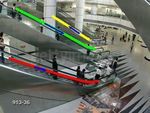
Figure 1. Elevator video: (a) flow vectors (yellow arrows) detected at the corresponding frames
#1, #101; (b) detected super tracks; (c) the motion flow field; (d) a sink seeking process; (e)
sink clustering.
scenes. In contrast, we are proposing a new method to optical flow for all pixel ([11]) in each frame. Con-
detect motion patterns in challenging crowded scenes sider a point i in the given frame. Its flow vector, Zi ,
where long-term tracks of moving objects are not avail- includes the location, Xi = (xi , yi ), and the velocity,
able or not reliable. In trajectory analysis, sinks are de- Vi = (vxi , vyi ), i.e., Zi = (Xi , Vi ). Note that, these
fined as the endpoints of paths and can be learned from flow vectors do not necessarily belong to foreground
the start and end points of the trajectories [2, 4]. How- objects and no time order or object labels are associated
ever, fragmented trajectories resulting from occlusions with them. In case, trajectories are available but not
or tracking failures will result in false sinks. To detect reliable, e.g., broken trajectories, then the flow vectors
sinks in this case, Stauffer [6] defined a transition likeli- can be obtained directly from these fragmented pieces
hood matrix and iteratively optimized the matrix for the of trajectories.
estimation of sources/sinks. Wang et al. [9] estimated
the sinks using the local density velocity map in a tra- All the flow vectors computed from all the frames
jectory clustering. In this paper, the sinks are defined as of the given video then constitute the global motion
the end points of the sink paths. They are the modes of flow field representing the instantaneous motion field
motion patterns and define the number of distinct mo- of the video. This flow field may contain thousands
tion patterns. of flow vectors and it is computational expensive to
apply sink seeking process to such a large amount of
2. Global Motion Flow Field Generation data. Moveover, these flow vectors always contain
redundant information and noise. Therefore, the flow
Given an input video, for each frame we use the ex- vectors belonging to the background can be considered
isting methods to compute sparse optical flow (instanta- as noise as they contain little motion information. To
neous velocities) using the interest points ([8]) or dense achieve this, we first apply a threshold on the velocitymagnitude to remove the flow vectors that have little
motion information. Next, we use Gaussian ART
(see [13]) to reduce the number of flow vectors from
thousands to hundreds. The reduced number of flow
vectors still maintain the geometric structure of the
flow field, and, therefore, do not effect the results of
detecting motion patterns. Fig. 1 shows example flow
vectors and corresponding motion flow field.
(a)
Sink Seeking: Suppose {Z1 , Z2 , · · · , Zn } is
the motion flow field where Zi = (Xi , Vi ). The states
of the sink seeking process of each point, i, are defined
as, Zei,t = (X ei,t , Vei,t ), t = 1, 2, ..., and computed
using:
Zei,1 = Zi , Xei,t+1 = Xei,t + Vei,t , (1) L⊥
P L //
ei,t ) Vn Wt,n
n∈N eighbor(X
Vei,t = P . (2)
n∈N eighbor(Xei,t ) Wt,n
The above equations states that the new ‘position’ of (b)
a point depends only on its location and velocity at the
last state. While the new ‘velocity’, Vei,t+1 , depends not Figure 2. Sink seeking process for a given
only on the previous velocity but also on the observed point. (a) sink seeking (red: the states of
velocities of its neighbors. See Fig. 2(b) which shows the flow vector in the sink seeking pro-
the motion trend of group of points in a local neighbor- cess, orange: the sink, rectangles: slid-
hood. In this paper, we employ the kernel based estima- ing windows, yellow: the sink path); (b)
tion similar to the mean shift approach [14] to incorpo- sliding window (solid circle: the flow vec-
rate this neighborhood effect using following equation: tor under consideration; rectangle: slid-
µ °e ° ¶ ing window; hollow circles: neighboring
° Vi,t−1 − Vn °2
Wt,n °
= exp −° ° , (3) points; dotted circles: non-neighboring
ht−1 °
points).
where ht−1 is the bandwidth. Note that, in the mean
shift tracking [14], the appearance of pixels in a small given a sink Zi∗ = (Xi∗ , Vi∗ ) associated with a sink
neighborhood around the object is used to determine path PZi∗ , and a cluster Ck , the sink-cluster distances
the location of the object in the next frame. In our ap- are given by: i) Dx (Zi∗ , Ck ) = maxZj∗ ∈Ck kXi∗ −
proach, we use the location and the velocity of neigh-
Xj∗ k, ii) Dv (Zi∗ , Ck ) = minZj∗ ∈Ck kVi∗ kkVj∗ k , iii)
boring points in the global flow field to determine the
next location. The pictorial description of the sink seek- Dp (Zi∗ , Ck )= maxZj∗ ∈Ck HausdorffDist(PZi∗ , PZj∗ ).
ing process is presented in Fig. 2(a). Here all metrics are based on comparison between
the given sink Zi∗ and the other sink Zj∗ in the cluster
3. Super Track Extraction Ck . The first metric measures whether the given sink
Zi∗ is spatially close to the cluster Ck or not. The sec-
After the sinks are obtained the next task is to clus- ond metric measures the similarity of their directions,
ter the sinks and determine their corresponding sink and the third measures the Hausdorff distance between
paths. The clustering algorithm starts by initializing their corresponding sink paths represented by PZi∗ and
the sink cluster set to an empty set. It takes each sink PZj∗ respectively. These three metrics ensure that two
and attempts to match it with all existing clusters. If flow vectors involved in a similar motion pattern have
a match is found, the sink is assigned to the matched similar sinks and sink paths. Following the clustering
cluster. Otherwise a new cluster is initialized with of sinks, for each cluster a super track is extracted as
the current sink as its center. Clusters with a small the sink path with the maximum arc length to represent
number of sinks are often caused by the background the corresponding global motion pattern (see Fig. 1).
or noise, and, therefore, are discarded. Formally,Figure 3. Generating super tracks for
crowd videos. Left Col: Extracted flow
vectors (yellow arrows). Center Col: The
motion flow field. Right Col: Detected su-
per tracks.
Super Track Matching: Each super track may
represent motions of several different objects (people,
cars etc), since they are generated using global flow
field of the whole video. Therefore, super tracks are
different form the traditional object tracks representing Figure 4. Super tracks in aerial video. (a)
the locations of a single object in different frames. Top: Initial tracking results where 6 cars
Super track can be used in video matching since they generated 16 broken tracklets. Middle:
can effectively reduce the problem of multi-object Trajectories superimposed on the video
multi-event video matching to the problem of matching mosaic. Bottom: Correctly generated sin-
two sets of super tracks. Consider two videos X and gle super track. (b) Left: Flow vectors su-
Y , and assume X and Y respectively have n and m perimposed on the mosaic. Right: Three
super tracks {xi }i=1,2,...,n and {yj }j=1,2,...,m . We super tracks. (c) Top: Flow vectors. Bot-
first define the similarity between two super tracks tom: Five super tracks.
(wi +w
Pj ) exp{−d(xi ,yj )} ,
xi and yj as p(xi , yj ) = (wi +wj )
i,j
where d(xi , yj ) is the shape distance computed by Crowd Videos: Fig. 1 shows a crowded scene
performing the dynamic time warping of the directional of a supermarket where crowds of people go up and
vectors of xi and yj (see [7] for details), and wi is the down through three escalators. Here, we used KLT
reliability weight associated to each track xi , which to extract initial flow vectors, and correctly generated
is given by wi = PnArcLength(x i)
. To find the three super-tracks corresponding to the motion patterns
k=1 ArcLength(xk )
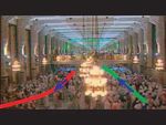
of three escalators. Fig. 3 shows results on two other
best matching between two groups: {xi }i=1,2,...,n
challenging sequence containing dense crowd. In
and {yj }j=1,2,...,m , we use maximum bipartite graph
Fig. 3(top-row), the crowd of pilgrims is moving in
matching to achieve where each super track is a node in
two opposite directions. The pilgrims are wearing
the bipartite graph. The weight of an edge between two
clothes of similar color and are occluded by each other,
nodes is given by the above equation. Given a bipartite
which makes it very hard to detect and track individual
graph G = (V, E), a matching M is a subset of E
persons. By processing this video through our proposed
such that for any two different members e, e0 ∈ M ,
method, we generated two super tracks which correctly
e ∩ e0 = ®. The maximum weight matching is the one
correspond to the two motion patterns: pilgrims going
that maximizes the sum of the weights.
up and pilgrims going down. Fig. 3(bottom-row)
4. Experiments demonstrates the strength of our method on a sequence
of an outdoor scene containing crowd and shadows. In
Two classes of videos are considered for the experi- this case several super tracks were extracted from the
ments which are i) Crowd, and ii) Aerial videos. These motion flow field. Again they correctly correspond to
videos contain groups of people and vehicles moving the running routes and the direction of motion.
mostly in an unconstrained setting in the presence of
shadows and severe occlusions. Aerial Videos: The aerial videos were taken from
DARPA’s VIVID data set. Here, the main challenge isto resolve the issue of broken trajectories resulting from
the limited field of view and occlusion of objects due to
terrain features. Initial tracklets were generated using
mean-shift tracker in motion compensated imagery.
The point flows are then extracted from these tracklets.
The first result is shown in Fig. 4(a) where super track
is extracted from the video showing a group of cars
making a U-turn. In this video, six vehicles move on
a highway in a convoy form, but only three or four of
them are captured by the camera at any time. Some cars
disappear for more than 100 frames and then reappear
which results in trajectories which are broken into
many tracklets. It is very difficult for a tracking based
approaches to detect the motion pattern from these
broken trajectories. In contrast, our method obtains
the flow vectors from these tracklets and does not use
the labels of objects, and, therefore, does not require
a complete trajectory. By applying our algorithm,
we are able to generate one super track representing
the motion patterns hidden in the 16 tracklets of this
Figure 5. First Row: Frames #500, #1000,
sequence. Two more results are shown in Fig. 4(b) and
#1130 of the query video. Second to
(c).
Fourth Row: Most similar videos with
scores of 0.88, 0.76 and 0.75 respectively.
Super Track Matching: We also tested the pro-
posed method for super track based video matching us- ECCV, 2004.
ing the VIVID data set consisting of 21 videos. Given a [2] D. Makris and T. Ellis, Automatic Learning of an
query video, the super tracks were generated using the Activity-based Semantic Scene Model, AVSBS, 2003.
proposed method. The super tracks of the query video [3] D. Makris and T. Ellis, Path Detection in Video Sequence,
were then compared with the super-track of each video IVC, Vol. 30, 2002.
in the database. Fig. 5 illustrates the video matching [4] S. McKenna et al., Learning Spatial Context from Track-
results for the sequence shown at the top which is an ing Using Penalised Likelihood Estimation, ICPR, 2004.
[5] N. Johnson et al., Learning the Distribution of Object
IR video. In this video, there was a group of cars mak-
Trajectories for Event Recognition, IVC, 14, 1996.
ing “S-turns” (see first row in Fig. 5). Fig. 5 shows
[6] C. Stauffer, Estimating Tracking Sources and Sinks,
the three videos with the greatest similarity to the query Event Mining Workshop, 2003.
video. Note that even though there are multiple groups [7] M. Vlachos et al., Rotation Invariant Distance Measures
of objects in these three videos and only one group in for Trajectories, SIGKDD, 2004.
the query video, all of them contain the same motion [8] B. D. Lucas and T. Kanade, An Iterative Image Regis-
pattern i.e. the S-turn. Despite the imperfect tracking tration Technique with an Application to Stereo Vision,
and the variability in path shapes, our method success- IJCAI, 1981.
fully matched the videos with the query video. [9] X. Wang et al., Learning Semantic Scene Models by Tra-
jectory Analysis, ECCV, 2006.
5. Conclusions [10] N. Vaswani et al., Activity Recognition Using the Dy-
namics of the Configuration of Interacting Objects,
We have proposed a new method based on instan-
CVPR, 2003.
taneous motion information, to detect typical motion [11] R. Gurka et al., Computation of Pressure Distribution
patterns for dense crowded scenes. This is achieved by Using PIV Velocity Data, Workshop on Particle Image
proposing a new construct called ‘super track’. Velocimetry, 1999.
[12] W. E. L. Grimson et al., Using Adaptive Tracking to
Acknowledgements: This research was funded Classify and Monitor Activities in a Site, CVPR, 1998.
by the US Government VACE program. [13] J. R. Williamson, Gaussian ARTMAP: A Neural Net-
work for Fast Incremental Learning of Noisy Multidimen-
References sional Maps, Neural Netw., 1996.
[14] D. Comaniciu et al., Mean Shift: A Robust Approach
[1] F. M. Porikli, Trajectory Pattern Detection by HMM Toward Feature Space Analysis, PAMI, 24(5). 2002.
Parameter Space Features and Eigenvector Clustering,You can also read


