Design of Amorphous Carbon Coatings Using Gaussian Processes and Advanced Data Visualization
←
→
Page content transcription
If your browser does not render page correctly, please read the page content below

lubricants
Article
Design of Amorphous Carbon Coatings Using Gaussian
Processes and Advanced Data Visualization
Christopher Sauer * , Benedict Rothammer                        , Nicolai Pottin, Marcel Bartz, Benjamin Schleich
and Sandro Wartzack

                                          Engineering Design, Friedrich-Alexander-Universität Erlangen-Nürnberg, Martensstraße 9,
                                          91058 Erlangen, Germany; rothammer@mfk.fau.de (B.R.); nicolai.pottin@fau.de (N.P.); bartz@mfk.fau.de (M.B.);
                                          schleich@mfk.fau.de (B.S.); wartzack@mfk.fau.de (S.W.)
                                          * Correspondence: sauer@mfk.fau.de

                                          Abstract: In recent years, an increasing number of machine learning applications in tribology and
                                          coating design have been reported. Motivated by this, this contribution highlights the use of Gaussian
                                          processes for the prediction of the resulting coating characteristics to enhance the design of amorphous
                                          carbon coatings. In this regard, by using Gaussian process regression (GPR) models, a visualization of
                                          the process map of available coating design is created. The training of the GPR models is based on the
                                          experimental results of a centrally composed full factorial 23 experimental design for the deposition
                                          of a-C:H coatings on medical UHMWPE. In addition, different supervised machine learning (ML)
                                          models, such as Polynomial Regression (PR), Support Vector Machines (SVM) and Neural Networks
                                          (NN) are trained. All models are then used to predict the resulting indentation hardness of a complete
                                          statistical experimental design using the Box–Behnken design. The results are finally compared, with
                                          the GPR being of superior performance. The performance of the overall approach, in terms of quality
                                          and quantity of predictions as well as in terms of usage in visualization, is demonstrated using an
                                          initial dataset of 10 characterized amorphous carbon coatings on UHMWPE.


                                          Keywords: machine learning; amorphous carbon coatings; UHWMPE; total knee replacement;
Citation: Sauer, C.; Rothammer, B.;
                                          Gaussian processes
Pottin, N.; Bartz, M.; Schleich, B.;
Wartzack, S. Design of Amorphous
Carbon Coatings Using Gaussian
Processes and Advanced Data
Visualization. Lubricants 2022, 10, 22.
                                          1. Introduction
https://doi.org/10.3390/                       Machine Learning (ML) as a subfield of artificial intelligence (AI) has become an
lubricants10020022                        integral part of many areas of public life and research in recent years. ML is used to create
Received: 14 December 2021
                                          learning systems that are considerably more powerful than rule-based algorithms and
Accepted: 3 February 2022
                                          are thus predestined for problems with unclear solution strategies and a high number of
Published: 7 February 2022
                                          variants. ML algorithms are used from product development and production [1] to patient
                                          diagnosis and therapy [2]. ML algorithms are also playing an increasingly important role
Publisher’s Note: MDPI stays neutral
                                          in the field of medical technology, for example, in coatings for joint replacements.
with regard to jurisdictional claims in
                                               Particularly in coating technology and design, the use of ML algorithms enables the
published maps and institutional affil-
                                          identification of complex relationships between several deposition process parameters on
iations.
                                          the process itself as well as on the properties of the resulting coatings [3,4]. From this view
                                          on the complex relationships between the deposition process parameters, coating designers
                                          can base their experiments and obtain valuable insights on their coating designs and the
Copyright: © 2022 by the authors.
                                          necessary parameter settings for coating deposition.
Licensee MDPI, Basel, Switzerland.             This contribution looks into the application of a possible ML algorithm in the coat-
This article is an open access article    ing design of amorphous carbon coatings. It first provides an overview of the necessary
distributed under the terms and           experimental setup for data generation and the concept of machine learning and its al-
conditions of the Creative Commons        gorithms. Likewise, the deposition of amorphous carbon coatings and their properties
Attribution (CC BY) license (https://     are presented. Subsequently, the capabilities of the selected supervised ML algorithms:
creativecommons.org/licenses/by/          Polynomial Regression (PR), Support Vector Machines (SVM), Neural Networks (NN),
4.0/).                                    Gaussian Process Regression (GPR) are explained and the resulting data visualization is

Lubricants 2022, 10, 22. https://doi.org/10.3390/lubricants10020022                                        https://www.mdpi.com/journal/lubricants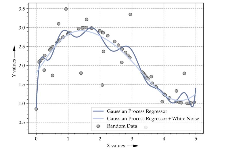
Lubricants 2022, 10, 22                                                                                           2 of 15

                          shown. Afterwards, the obtained results are discussed, with the GPR being the superior
                          prediction model. Finally, the main findings are summarized and an outlook is given as
                          well as further potentials and applications are identified.

                          2. Related Work and Main Research Questions
                          2.1. Amorphous Carbon Coating Design
                                An example of a complex process is the coating of metal and plastic parts, as used
                          for joint replacements, with amorphous carbon coatings [5]. In the field of machine
                          elements [6,7], engine components [8,9] and tools [10,11], amorphous carbon coatings are
                          commonly used. In contrast, amorphous carbon coatings are rarely used for load-bearing,
                          tribologically stressed implants [12,13]. The coating of engine and machine elements has so
                          far been used with the primary aim of reducing friction, whereas the coating of forming
                          tools has been used to adjust friction while increasing the service life of the tools. There-
                          fore, the application of tribologically effective coating systems on the articulating implant
                          surfaces is a promising approach to reduce wear and friction [14–16].
                                The coating process depends on many different coating process parameters, such as
                          the bias voltage [17], the target power [18], the gas flow [19] or the temperature, which
                          influence the chemical and mechanical properties as well as the tribological behavior of the
                          resulting coatings [20]. Therefore, it is vital to ensure both the required coating properties
                          and a robust and reproducible coating process to meet the high requirements for medical
                          devices. Compared to experience-based parameter settings, which are often based on
                          trial-and-error, ML algorithms provide clearer and more structured correlations.
                                However, several experimental investigations focus on improving the tribological
                          effectiveness of joint replacements [21–23] and lubrication conditions in prostheses [24–26],
                          some experimental investigations are complemented with computer-aided or computa-
                          tional methods to improve the prediction and findings [27–29]. Nevertheless, the exact
                          interactions of coating process parameters and resulting properties are mostly qualitative
                          and only valid for certain coating plants and in certain parameter ranges.

                          2.2. Coating Process and Design Parameters
                               The use of ML algorithms is a promising approach [30] to not only qualitatively
                          describe such interactions, which have to be determined in elaborate experiments, but
                          also to quantify them [21]. Using ML, the aim is to generate reproducible, robust coating
                          processes with appropriate, required coating properties. For this purpose, the main coating
                          properties, such as coating thickness, roughness, adhesion, hardness and indentation
                          modulus, of the coating parameter variations have to be analyzed and trained with suitable
                          ML algorithms [31].
                               Within this contribution, the indentation modulus and the coating hardness are ex-
                          amined in more detail, since these parameters can be determined and reproduced with
                          high accuracy and have a relatively high predictive value for the subsequent tribological
                          behavior, such as the resistance to abrasive wear [32,33].

                          2.3. Research Questions
                                Resulting from the above-mentioned considerations it was found that existing solu-
                          tions are solely based on a trial-and-error approach. ML was not considered in the specific
                          coating design in joint replacements. So, in brief, this contribution wants to answer the
                          following central questions. The first one is can ML algorithms predict resulting properties
                          in amorphous carbon coatings? Based on this, the second one is how good is the resulting
                          prediction of resulting properties in terms of quality and quantity? And lastly, can ML
                          support in visualizing the coating properties results and the coating deposition parameters
                          leading to those results? When ML can be used in these cases, the main advantages would
                          be a more efficient approach to coating design with fewer to none trial-and-error steps and,
                          lastly, the co-design of coating experts and ML. The following sections are to present the
Lubricants 2022, 10, 22                                                                                           3 of 15

                          materials and methods used in trying to answer the stated research questions and provide
                          an outlook on what would be possible via ML.

                          3. Materials and Methods
                               First, the studied materials and methods will be described briefly. In this context,
                          the application of the amorphous carbon coating to the materials used (UHMWPE) as
                          well as the setup and procedure of the experimental tests to determine the mechanical
                          properties (hardness and elasticity) are described. Secondly, the pipeline for ML and the
                          used methods are explained. Finally, the programming language Python and the deployed
                          toolkits are described.

                          3.1. Experimental Setup
                          3.1.1. Materials
                                The investigated substrate was medical UHMWPE [34] (Chirulen® GUR 1020, Mit-
                          subishi Chemical Advanced Materials, Vreden, Germany). The specimens to be coated were
                          flat disks, which have been used for mechanical characterization (see [35]). The UHMWPE
                          disks had a diameter of 45 mm and a height of 8 mm. Before coating, the specimens
                          were mirror-polished in a multistage polishing process (Saphir 550-Rubin 520, ATM Qness,
                          Mammelzen, Germany) and cleaned with ultrasound (Sonorex Super RK 255 H 160 W
                          35 Hz, Bandelin electronic, Berlin, Germany) in isopropyl alcohol.

                          3.1.2. Coating Deposition
                                Monolayer a-C:H coatings were prepared on UHMWPE under two-fold rotation using
                          an industrial-scale coating equipment (TT 300 K4, H-O-T Härte- und Oberflächentech-
                          nik, Nuremberg, Germany) for physical vapor deposition and plasma-enhanced chemi-
                          cal vapor deposition (PVD/PECVD). The recipient was evacuated to a base pressure of
                          at least 5.0 × 10⁻⁴ Pa before actual deposition. The recipient was not preheated before
                          deposition on UHMWPE to avoid the deposition-related heat flux into UHMWPE. The
                          specimens were then cleaned and activated for 2 min in an argon (Ar, purity 99.999%)+ -ion
                          plasma with a bipolar pulsed bias of −350 V and an Ar flow of 450 sccm. The deposition
                          time of 290 min was set to achieve a resulting a-C:H coating thickness of approximately
                          1.5 to 2.0 µm. Using reactive PVD, the a-C:H coating was deposited by medium frequency
                          (MF)-unbalanced magnetron (UBM) sputtering of a graphite (C, purity 99.998%) target
                          under Ar–ethyne (C2 H2 ) atmosphere (C2 H2 , purity 99.5%). During this process, the cathode
                          (dimensions 170 × 267.5 mm) was operated with bipolar pulsed voltages. The negative
                          pulse amplitudes correspond to the voltage setpoints, whereas the positive pulses were
                          represented by 15% of the voltage setpoints. The pulse frequency f of 75 kHz was set
                          with a reverse recovery time RRT of 3 µs. A negative direct current (DC) bias voltage was
                          used for all deposition processes. The process temperature was kept below 65 ◦ C during
                          the deposition of a-C:H functional coatings on UHMWPE. In Table 1, the main, varied
                          deposition process parameters are summarized. Besides the reference coating (Ref), the
                          different coating variations (C1 to C9) of a centrally composed full factorial 23 experimental
                          design are presented in randomized run order. In this context, the deposition process
                          parameters shown here for the generation of different coatings represent the basis for the
                          machine learning process.
Lubricants 2022, 10, 22 4 of 15
Table 1. Summary of the main deposition process parameters for a-C:H on UHMWPE.
Sputtering Bias Combined Ar and
Designation Coating
Power/kW Voltage/V C2 H2 Flow/sccm
Ref 0.6 −130 187
C1 0.6 −90 187
C2 2.0 −170 91
C3 1.3 −130 133
C4 2.0 −90 187
a-C:H
C5 0.6 −170 91
C6 2.0 −170 187
C7 0.6 −170 187
C8 0.6 −90 91
C9 2.0 −90 91
3.1.3. Mechanical Characterization
According to [36,37], the indentation modulus EIT and the indentation hardness HIT
were determined by nanoindentation with Vickers tips (Picodentor HM500 and WinHCU,
Helmut Fischer, Sindelfingen, Germany). For minimizing substrate influences, care was
taken to ensure that the maximum indentation depth was considerably less than 10% of the
coating thicknesses [38,39]. Considering the surface roughness, lower forces also proved
suitable to obtain reproducible results. Appropriate distances of more than 40 µm were
maintained between individual indentations. For statistical reasons, 10 indentations per
specimen were performed and evaluated. A value for Poisson’s ratio typical for amorphous
carbon coatings was assumed to determine the elastic–plastic parameters [40,41]. The
corresponding settings and parameters are shown in Table 2. In Section 3, the results of
nanoindentation are presented and discussed.
Table 2. Settings for determining the indentation modulus EIT and the indentation hardness HIT .
Parameters Settings for a-C:H Coatings
Maximum load/mN 0.05
Application time/s 3
Delay time after lowering/s 30
Poisson’s ratio ν 0.3
3.2. Machine Learning and Used Models
3.2.1. Supervised Learning
The goal of machine learning is to derive relationships, patterns and regularities from
data sets [42]. These relationships can then be applied to new, unknown data and problems
to make predictions. ML algorithms can be divided into three subclasses: supervised,
unsupervised and reinforced learning. In the following, only the class of supervised
learning will be discussed in more detail, since algorithms from this subcategory were used
in this paper, namely Gaussian process regression (GPR). Supervised ML was used because
of the available labelled data.
In supervised learning, the system is fed classified training examples. In this data, the
input values are already associated with known output data values. This can be done, for
example, by an already performed series of measurements with certain input parameters
(input) and the respective measured values (output). The goal of supervised learning is to
train the model or the algorithms using the known data in such a way that statements and
predictions can also be made about unknown test data [42]. Due to the already classified
data, supervised learning represents the safest form of machine learning and is therefore
very well suited for optimization tasks [42].
In the field of supervised learning, one can distinguish between the two problem types
of classification and regression. In a classification problem, the algorithm must divide the
data into discrete classes or categories. In contrast, in a regression problem, the model is toLubricants 2022, 10, 22 5 of 15
estimate the parameters of pre-defined functional relationships between multiple features
in the data sets [42,43].
A fundamental danger with supervised learning methods is that the model learns the
training data by role and thus learns the pure data points rather than the correlations in data.
As a result, the model can no longer react adequately to new, unknown data values. This
phenomenon is called overfitting and must be avoided by choosing appropriate training
parameters [31]. In the following, basic algorithms of supervised learning are presented,
ranging from PR and SVM to NN and GPR.
3.2.2. Polynomial Regression
At first, we want to introduce polynomial regression (PR) for supervised learning. PR
is a special case of linear regression and tries to predict data with a polynomial regression
curve. The parameters of the model are often fitted using a least square estimator and the
overall approach is applied to various problems, especially in the engineering domain. A
basic PR model can lead to the following equation [44]:
yi = β0 + β1 xi1 + β2 xi2 + . . . + βk xik +ei for i = 1, 2, . . . , n (1)
with β being the regression parameters and e being the error values. The prediction targets
are formulated as yi and the features used for prediction are described as xi . A more
sophisticated technique based on regression models are support vector machines, which
are described in the next section.
3.2.3. Support Vector Machines
Originally, support vector machines (SVM) are a model commonly used for classi-
fication tasks, but the ideas of SVM can be extended to regression as well. SVM try to
find higher order planes within the parameter space to describe the underlying data [45].
Thereby, SVM are very effective in higher dimensional spaces and make use of kernel
functions for prediction. SVM are widely used and can be applied to a variety of problems.
In this regard, SVM can also be applied nonlinear problems. For a more detailed theoretical
insight, we refer to [45].
3.2.4. Neural Networks
Another supervised ML technique is neural networks (NN), which rely on the concept
of the human brain to build interconnected multilayer perceptrons (MLP) capable of
predicting arbitrary feature–target correlations. The basic building block of such MLP
are neurons based on activation functions which allow the neuron to fire when different
threshold values are reached [46]. When training a NN, the connections and the parameters
of those activation functions are optimized to minimize training errors; this process is called
backpropagation [31].
3.2.5. Gaussian Process Regression
The Gaussian processes are supervised generic learning methods, which were devel-
oped to solve regression and classification problems [43]. While classical regression algo-
rithms apply a polynomial with a given degree or special models like the ones mentioned
above, GPR uses input data more subtly [47]. Here, the Gaussian process theoretically
generates an infinite number of approximation curves to approximate the training data
points as accurately as possible. These curves are assigned probabilities and Gaussian
normal distributions, respectively. Finally, the curve which fits its probability distribution
best to that of the training data is selected. In this way, the input data gain significantly
more influence on the model, since in the GPR altogether fewer parameters are fixed in
advance than in the classical regression algorithms [47]. However, the behavior of the
different GPR models can be defined via kernels. This can be used, for example, to influence
how the model should handle outliers and how finely the data should be approximated.Lubricants 2022, 10, x FOR PEER REVIEW 6 of 16
Lubricants 2022, 10, 22 advance than in the classical regression algorithms [47]. However, the behavior of the dif- 6 of 15
ferent GPR models can be defined via kernels. This can be used, for example, to influence
how the model should handle outliers and how finely the data should be approximated.
In Figure 1, two different GPR models have been used to approximate a sinusoid.
In Figure 1, two different GPR models have been used to approximate a sinusoid. The
The input data points are sinusoidal but contain some outliers. The model with the
input data points are sinusoidal but contain some outliers. The model with the lightblue
lightblue approximation curve has an additional kernel extension for noise suppression
approximation curve has an additional kernel extension for noise suppression compared to
compared to the darkblue model. Therefore, the lightblue model is less sensitive to outli-
the darkblue model. Therefore, the lightblue model is less sensitive to outliers and has a
erssmoother
and has aapproximation
smoother approximation
curve. This curve.
is also This is also
the main the mainwhen
advantage advantage whencompared
using GPR using
GPR compared to other regression models like linear or polynomial regression.
to other regression models like linear or polynomial regression. GPR are more robust GPR are to
more robust to outliers or messy data and are also relatively stable on small datasets
outliers or messy data and are also relatively stable on small datasets [47] like the one [47]
likeused
the one usedcontribution.
for this for this contribution. Thatthey
That is why is why
werethey were mainly
mainly selectedselected
for the for the later-
later-described
described
use case. use case.
Figure
Figure 1. Gaussian
1. Gaussian process
process regression
regression for for
thethe regression
regression of aofsinusoid.
a sinusoid.
3.2.6. Python
3.2.6. Python
The Python programming language was chosen for the present work, as it is the
The Python
de-facto programming
standard language for language
ML and was
Datachosen for the
Science. Thispresent work, asenvironment
programming it is the de- is
facto standard language for ML and Data Science. This programming environment
particularly suitable in the field of machine learning, as it allows the easy integration is par- of
ticularly
externalsuitable in the
libraries. field of
In order tomachine learning,
use machine as italgorithms
learning allows the ineasy integration
practice, manyof ex-
libraries
ternal
andlibraries.
environmentsIn order
have tobeen
use machine
developed learning algorithmsOne
in the meantime. in practice,
of them ismany libraries
the open-source
andPython
environments have been developed
library scikit-learn in the
[48]. For the meantime. Onemethods,
above-described of them isthethefollowing
open-source scikit-
Python library scikit-learn [48]. For the above-described methods, the following
learn libraries were used: the scikit-learn module Polynomial Features for the modeling scikit-
learn libraries
of the were used:
PR models, which thewasscikit-learn
combined module
with thePolynomial Features for
Linear Regression the modeling
module to facilitate
of the
a PRPRmodel
models,forwhich was combined
prediction of coatingwith the LinearFor
parameters. Regression
modeling module
via SVM,to facilitate
the SVR a or
PR support
model for prediction
vector of coating
regressor module parameters. For modeling
of scikit-learn was used.via The SVM,
NN the
were SVR or support
modeled via the
vector
MLPregressor
Regressormodule
moduleofand scikit-learn
lastly the was
GPRused. The NN wereusing
were implemented modeled via the MLP
the Gaussian Process
Regressor
Regressor module
moduleandoflastly the GPRAll
scikit-learn. were implemented
models were trainedusing the the
using Gaussian
standard Process Re-
parameters,
gressor module
and only of scikit-learn.
for the GPR modelAll models
was werefunction
the kernel trained using the standard
smoothed via adding parameters,
some white
andnoise;
only this
for the
wasGPR modelbecause
necessary was thethe kernel
GPR of function smoothed
scikit-learn has novia adding
real standardsome white
parameters.
noise; this was necessary because the GPR of scikit-learn has no real standard parameters.
4. Use Case with Practical Example in a-C:H Coating Design
4.1. Case
4. Use Data Generation
with Practical Example in a-C:H Coating Design
4.1. DataThe average indentation modulus and indentation hardness values are presented
Generation
in Figure 2 Obviously, elasticity and hardness differed significantly between the various
The average indentation modulus and indentation hardness values are presented in
coated groups. A considerable influence of the sputtering power on the achieved EIT and
Figure 2 Obviously, elasticity and hardness differed significantly between the various
HIT values was revealed. For example, C2, C4, C6 and C9, which were produced with
coated groups. A considerable influence of the sputtering power on the achieved EIT and
a sputtering power of 2.0 kW, had indentation modulus between 13.3 and 16.4 GPa and
HIT values was revealed. For example, C2, C4, C6 and C9, which were produced with a
indentation hardness between 3.7 and 5.1 GPa. In contrast, specimens Ref, C1, C5, C7 and
sputtering power of 2.0 kW, had indentation modulus between 13.3 and 16.4 GPa and
C8 exhibited significantly lower EIT and HIT values, ranging from 3.6 to 4.9 GPa and 1.2 to
1.5 GPa, respectively. Compared to the latter, the central point represented by C3 did not
indicate significantly higher elastic–plastic values. The variation of the bias voltage or the
combined gas flow did not allow us to derive a distinct trend, especially concerning theindentation hardness between 3.7 and 5.1 GPa. In contrast, specimens Ref, C1, C5, C7 and
C8 exhibited significantly lower EIT and HIT values, ranging from 3.6 to 4.9 GPa and 1.2 to
1.5 GPa, respectively. Compared to the latter, the central point represented by C3 did not
Lubricants 2022, 10, 22 indicate significantly higher elastic–plastic values. The variation of the bias voltage or the 7 of 15
combined gas flow did not allow us to derive a distinct trend, especially concerning the
standard deviation. In general, increased sputtering power could increase EIT and HIT by
more than a factor
standard of three.
deviation. Accordingly,
In general, the higher
increased coating
sputtering hardness
power could is expected
increase EITtoand
shield
HIT by
the more
substrates from adhesive and abrasive wear and also to shift the cracking towards
than a factor of three. Accordingly, the higher coating hardness is expected to shield
higher
the stresses
substrates[28,35].
from At the same
adhesive time,
and the relatively
abrasive wear and lower
alsoindentation
to shift the modulus
cracking leads
towards
to an increased ability of the coatings to sag without flowing [33]. As a result,
higher stresses [28,35]. At the same time, the relatively lower indentation modulus the pressures
leads to
induced by tribological
an increased ability loading may be to
of the coatings reduced by increasing
sag without flowingthe contact
[33]. dimensions
As a result, [49].
the pressures
Thus, it can by
induced be considered
tribological that the developed
loading a-C:Hby
may be reduced coatings enable
increasing theacontact
very advantageous
dimensions [49].
wear behavior [28,50].
Thus, it can be considered that the developed a-C:H coatings enable a very advantageous
wear behavior [28,50].
Figure 2. Averaged values of indentation modulus EIT and indentation hardness HIT and standard
Figure 2. Averaged values of indentation modulus EIT and indentation hardness HIT and standard
deviation of the different a-C:H coatings (n = 10).
deviation of the different a-C:H coatings (n = 10).
4.2. Data Processing
4.2.4.2.1.
Data Processing
Reading in and Preparing Data
4.2.1. Reading in and
After the Preparing
coating Data
characterization, the measured values were available in a stan-
dardized
After theExcel dataset,
coating which contains
characterization, the plantvalues
the measured parameters and the resulting
were available coating
in a standard-
izedcharacteristics
Excel dataset,for each contains
which sample. Itthecould
plantalso be possible
parameters that
and thethe relevantcoating
resulting measurements
charac- are
already
teristics for in a machine-readable
each format,
sample. It could also for example
be possible the relevant
that the tribAIn ontology
measurements[51], but
arefor
al-our
case we focused on the data handling via Excel and Python. To facilitate
ready in a machine-readable format, for example the tribAIn ontology [51], but for our the import of the
data into Python, the dataset had to be modified in such a way that a column-by-column
case we focused on the data handling via Excel and Python. To facilitate the import of the
dataimport of the data
into Python, was possible.
the dataset had to Afterwards,
be modified in thesuch
dataset needed
a way that atocolumn-by-column
be imported into our
Python
import program
of the via possible.
data was the pandas library [52].the
Afterwards, Todataset
facilitate further
needed todata processing,
be imported the
into plant
our
Python program via the pandas library [52]. To facilitate further data processing, the plant in
parameters sputtering power, bias voltage and combined Ar and C 2 H 2 were combined
an arraysputtering
parameters of featurespower,
and the coating
bias characteristic
voltage and combined suchArasand
theCindentation hardness as a
2H2 were combined in
target for prediction.
an array of features and the coating characteristic such as the indentation hardness as a
target for prediction.
4.2.2. Model Instantiation
The class
4.2.2. Model Gaussian Process Regressor (GPR) of the scikit-learn package class allows the
Instantiation
implementation of Gaussian process models. For the instantiation in particular, a definition
The class Gaussian Process Regressor (GPR) of the scikit-learn package class allows
of a kernel was needed. This kernel is also called covariance function in connection with
the Gaussian
implementation of Gaussian
processes process
and influences themodels.
probabilityFor the instantiation
distributions in particular,
of the a def-
Gaussian processes
inition of a kernel was needed. This kernel is also called covariance function
decisively. The main task of the kernel is to calculate the covariance of the Gaussian in connection
with Gaussian
process processes
between the and influences
individual datathe probability
points. Two distributions
GPR objects of the instantiated
were Gaussian pro- with
cesses
two different kernels. The first one was created with a standard kernel andthe
decisively. The main task of the kernel is to calculate the covariance of theGaussian
second one
process between the individual
was additionally linked withdata points.
a white Twokernel.
noise GPR objects
Duringwere instantiated
the later with two the
model training,
different kernels. The of
hyperparameters first
theone was were
kernel created with a standard
optimized. Due tokernel andoccurring
possibly the second onemaxima,
local was
additionally linked with a white noise kernel. During the later model
the passing parameter n_restarts_optimizer can be used to determine how often training, the hy-this
perparameters of the kernel were optimized. Due to possibly occurring
optimization process should be run. In the case of GPR, a standardization of the local maxima, thedata
was carried out. This standardization was achieved by scaling the data mean to 0 and the
standard deviation to 1.
4.2.3. Training the Model
As described before, one of the main tasks of machine learning algorithms was the
training of the model. The scikit-learn environment offers the function fit(X,y), with theLubricants 2022, 10, 22 8 of 15
input variables X and y. Here, X was the feature vector, which contains the feature data of
the test data set (the control variables of the coating plant). The variable y was defined as
the target vector and contains the target data of the test data set (the characteristic values of
the coating characterization). By calling the method reg_model.fit(X,y) with the available
data and the selected regression model (GPR, in general reg_model) the model was trained
and fitted on the available data.
Particularly with small datasets, there was the problem that the dataset shrank even
further when the data was divided into training and test data. For this reason, the k-fold
cross-validation approach could be used [31]. Here, the training data set was split into k
smaller sets, with one set being retained as a test data set per training run. In the following
runs, the set distributions change. This approach can be used to obtain more training
datasets despite small datasets, thus significantly improving the training performance of
the model.
4.2.4. Model Predictions
After the models were trained on the available data, the models can compute or predict
corresponding target values for the feature variables that were previously unknown to
the model. Unknown feature values are equally distributed data points from a specified
interval as well as the features of a test data set. For the former, the minima and maxima of
the feature values of the training data set were extracted. Afterwards, equally distributed
data points were generated for each feature in this min-max interval.
For predicting the targets, the scikit-learn library provides the method predict(x),
where the feature variables are passed as a vector x to the function. Calling the method
reg_model.predict(x) then returns the corresponding predicted target values. The predic-
tions for the test data were further evaluated in terms of the root mean squared error, the
mean absolute error and the coefficient of prognosis (CoP) [53] and showed good quality,
especially for the GPR model (see Table 3).
Table 3. Prediction quality of the models based on the initial dataset.
Root Mean Mean Absolute Coefficient of
Model
Squared Error Error Prognosis
Gaussian Process Regressor 540 MPa 474 MPa 91%
Polynomial Regression 699 MPa 653 MPa 45%
Support Vector Machine 955 MPa 677 MPa 29%
Neural Network 3405 MPa 3307 MPa 16%
From Table 3, it follows that the GPR model is the most suitable model for further
evaluation in our test case since it shows the highest coefficient of prognosis. Therefore, we
selected the GPR model for the demonstration and visualization of our use case.
4.2.5. Visualization
The Python library matplotlib was used to visualize the data in Python. This allowed
an uncomplicated presentation of numerical data in 2D or 3D. Since the feature vector
contained three variables (sputter power P sputter, gas flow ϕ and bias voltage Ubias ), a
three-dimensional presentation of the feature space was particularly suitable. Here, the
three variables were plotted on the x-, y- and z-axis and the measurement points were
placed in this coordinate system. For the presentation of the corresponding numerical
target value, color-coding serves as the fourth dimension. The target value of the measuring
point could then be inferred from a color bar.
This presentation was especially suitable for small data sets, e.g., to get an overview
of the actual position of the training data points. For large data sets with several thousand
data points, a pure 3D visualization is too confusing, since measurement points inside the
feature space were no longer visible. For this reason, a different visualization method was
used to display the results of ML prediction of uniformly distributed data.Lubricants 2022, 10, 22 9 of 15
This visualization method is based on the visualization of computer tomography (CT)
data set using a slice-based data view. Here, the 3D images of the body are skipped through
layer-by-layer to gain insights into the interior of the workings level-by-level. Similar to
this principle, the feature space was also traversed layer-by-layer.
Two feature variables span a 2D coordinate system. The measured values were again
colored and displayed in the x–y plane analogous to the 3D display.
The third feature vector served as a run variable in the z-axis, i.e., into the plane.
Employing a slider, the z-axis can be traversed, and the view of the feature space was then
obtained layer-by-layer.
5. Results and Discussion
5.1. Gaussian Process Regression and Visualization
For the above-described initial dataset created from a design of experiments approach,
different GPR models were trained. Before training the different models, the dataset was
scaled to only contain values between 0 and 1. This was especially useful for GPR, to reduce
training effort and stabilize the optimization of the model parameters. The main difference
between the different GPR models was the used kernel function for the gaussian processes.
The used GPR supports a variety of different kernel functions which were optimized during
the training of the GPR model. It was found that with a dot product kernel with some
additional white noise the prediction capabilities of the model were enhanced to reach
a mean absolute error of around 440 MPa. Moreover, the root mean squared error was
around 387 MPa. This results in an CoP of around 90%, which means that the prediction
quality and quantity is acceptable to classify this model for a prediction model. For model
training, a train-test-split of 80–20% was used and the training data was shuffled before
training. The overall prediction quality is a notable finding since the dataset used for
training is relatively small. Here also GPR with little white noise show their strengths on
sparse datasets. However, model performance can further benefit from more data. This
prediction model is also capable of visualizing the prediction space, see Figure 3.
U
MPa
Indentation Hardness
kW
Combined Ar and C2H2 flow 91 sccm
Figure 3. Predicted space in a 20-color colormap for better differentiation between the different areas
of resulting hardness for minimum combined gas flow.
The striped pattern emerges from the usage of a 20-color-based colormap for drawing.
This is done to further show the different sections of the predicted data. The whole plot
can be viewed as a process map. In order to find the ideal coating properties, the tribology
experts need to look for their color in indentation hardness and then easily see the bias
voltage and sputtering power needed. For tuning purposes, the gas flow can be changed
via the slider at the bottom. The plot for the maximum combined gas flow is depicted in
Figure 4.Lubricants 2022, 10, 22 10 of 15
U
MPa
Indentation Hardness
kW
Combined Ar and C2H2 flow 187 sccm
Figure 4. Predicted space for maximum combined gas flow.
The space for lower indentation hardness is getting bigger and the highest indentation
hardness of around 4.2 GPa vanished. This correlates with the experience made from
initial experimental studies. It was expected that the gas flow—especially the C2 H2 gas
flow [15]—influenced the hydrogen content and thus the mechanical properties and further
affected the tribologically effective behavior. Based on these visualizations, it can be
easily seen which parameters lead to the desired indentation hardness. This visualization
technique benefits the process of where to look for promising parameter sets for ideal
indentation hardness.
For validation of our model, we performed another experimental design study based
on a Box–Behnken design with 3 factors and two stages (see Table 4). Initially, the in-
dentation hardness was predicted using our GPR model. Subsequently, the GPR model
was evaluated—after coating the specimens—by determining the indentation hardness
experimentally. For illustrative purposes, the prediction of the central point, which was
deposited at a sputtering power of 3 kW, a bias voltage of 200 V, and a combined gas flow
of 108 sccm, is shown in Figure 5. In this context, it should be noted that the prediction
space included a significant extension of the training space and thus could be influenced
by many factors.
U
MPa
Indentation Hardness
Prediction of central point: 4576 MPa
X
kW
Combined Ar and C2H2 flow 108 sccm
Figure 5. Predicted extended space for probe points.Lubricants 2022, 10, 22 11 of 15
Table 4. Summary of main deposition process parameters and predictions for a-C:H on UHMWPE,
prediction of HIT by the GPR model as well as experimental determination of HIT based on the
average values and standard deviations of the different a-C:H coatings (n = 10).
GPR Model Experimentally
Sputtering Bias Combined Ar and
Designation Coating Prediction of Determined
Power/kW Voltage/V C2 H2 Flow/Sccm
H IT /MPa H IT /MPa
P1 2 −230 108 3397 3040 ± 223
P2 2 −170 108 3355 2441 ± 537
P3 2 −200 125 3363 3069 ± 401
P4 2 −200 91 3389 2965 ± 328
P5.1 3 −200 108 4576 4699 ± 557
P5.2 3 −200 108 4576 4577 ± 731
P5.3 3 −200 108 4576 4837 ± 634
P6 a-C:H 3 −170 125 4542 4180 ± 399
P7 3 −170 91 4568 4256 ± 622
P8 3 −230 125 4584 4627 ± 1055
P9 3 −230 91 4610 4415 ± 675
P10 4 −170 108 5755 5081 ± 1361
P11 4 −200 91 5789 5476 ± 1637
P12 4 −230 108 5797 4313 ± 1513
P13 4 −200 125 5763 6224 ± 1159
As shown in Figure 5 and Table 4, the HIT values of the previously performed predic-
tion of the GPR model largely coincided with the experimentally determined HIT values.
Especially with regard to the standard deviation of the experimentally determined HIT
values, all values were in a well-usable range for further usage and processing of the data.
Despite a similar training space, the prediction for the coating variations P1–P4 showed
a slightly lower accuracy than for the coating variations beyond the training space, but
this could be attributed to the difficulty of determining the substrate-corrected coating
hardness. Thus, during the indentation tests, the distinct influence of the softer UHMWPE
substrate [54,55] was more pronounced for the softer coatings (P1–P4), which were coated
with lower target power than for the harder coatings (P5–P13). However, the standard
deviation of the hardness values increased with hardness, which could be attributed to
increasing coating defects locations and roughness. In brief, the predictions match with
the implicit knowledge of the coating experts. This is the only physical conceivable con-
ceptual model that can be considered when looking at the results presented, as the coating
deposition is a complex and multi-scale process.
Though the visualization of the prediction space in Figure 5 differed slightly from the
prediction spaces in Figure 3 and in Figure 4 due to steeper dividing lines, the prediction
space in Figure 5 spanned larger coating process parameter dimensions.
Generally, the prediction quality and especially the quantity of the model was very
good, so the model can be used for further coating development processes and adjustments
of the corresponding coating process parameters. An extension of the GPR model to other
coating types, such as ceramic coatings, e.g., CrN, or solid lubricants, e.g., MoS2 , or different
coating systems on various substrates is conceivable.
5.2. Comparison to Polynomial Regression, Support Vector Machines and Neural Network Models
For the purpose of comparing our results and trained models with the other models
described previously, Table 5 shows the different predictions generated by the models for
the previously unknown dataset in our test study.Lubricants 2022, 10, 22 12 of 15
Table 5. Comparison of the predictions of the different models used in this contribution.
Experimentally GPR Model PR Model SVM Model NN Model
Designation Determined Prediction of Prediction of Prediction of Prediction of
H IT /MPa H IT /MPa H IT /MPa H IT /MPa H IT /MPa
P1 3040 ± 223 3397 3861 4220 1402
P2 2441 ± 537 3355 3566 4218 1153
P3 3069 ± 401 3363 3567 4219 1346
P4 2965 ± 328 3389 4101 4219 1209
P5.1 4699 ± 557 4576 4863 4219 1281
P5.2 4577 ± 731 4576 4863 4219 1281
P5.3 4837 ± 634 4576 4863 4219 1281
P6 4180 ± 399 4542 4548 4217 1225
P7 4256 ± 622 4568 4850 4218 1088
P8 4627 ± 1055 4584 5063 4219 1475
P9 4415 ± 675 4610 5376 4220 1336
P10 5081 ± 1361 5755 4912 4218 1160
P11 5476 ± 1637 5789 5447 4219 1216
P12 4313 ± 1513 5797 5659 4220 1409
P13 6224 ± 1159 5763 5366 4219 1354
It is shown that only the GPR model is capable of producing meaningful outputs,
while the other models are not able to achieve a prediction quality close to the GPR model.
When comparing the training results on root mean squared error, mean absolute error and
coefficient of prognosis set, the story becomes even more clearer (see Table 6).
Table 6. Comparison of the prediction qualities of the models on the unknown data set.
Root Mean Mean Absolute Coefficient of
Model
Squared Error Error Prognosis
Gaussian Process Regressor 551 MPa 415 MPa 78%
Polynomial Regression 720 MPa 587 MPa 71%
Support Vector Machine 991 MPa 781 MPa 0.1%
Neural Network 3156 MPa 2999 MPa 1%
The results show that the GPR model was the best model compared to PR, SVM and
NN. It is worth noting that we have used polynomial degree of 2 for the PR models, as
this produced the best prediction results, a higher polynomial degree of 3 to 5 led to a
decrease in RMSE, MAE and CoP. This also shows that especially the SVM and NN are
not capable of producing meaningful prediction output. The PR fitting overall shows
acceptable prediction quality of around 70%, however the GPR has better RMSE and MAE
values, so it would be selected for further consideration. Furthermore, GPR provided better
results on the training dataset. It is important to always evaluate RMSE, MAE and CoP
together, as all three values allow a thorough evaluation of the prediction model. In brief,
RMSE and MAE characterize the spread predictions better than the CoP, the CoP returns
an overall performance score of the model. The weak performance of SVM can possibly be
explained by the small dataset used for training, since SVM need way more training data,
as the model only scores around 30% CoP on the training dataset. For extrapolation on the
test dataset the trained SVM model was not feasible. The same could be the case for the
NN, as NN rely on big datasets for training and show weaker extrapolation capabilities.
6. Conclusions
This contribution evaluated the use of Gaussian processes and advanced data visu-
alization in the design of amorphous carbon coatings on UHMWPE. This study focused
on elaborating an overview of the required experimental setup for data generation andLubricants 2022, 10, 22 13 of 15
the concepts of ML, and also provided the corresponding ML algorithms. Afterwards, the
deposition and characterization of amorphous carbon coatings were presented.
The use of ML in coating technology and tribology represents a very promising ap-
proach for the selective optimization of coating process parameters and coating properties.
In particular, this could be demonstrated by the GPR models used to optimize the mechani-
cal properties of the coatings and, consequently, the tribological behavior, by increasing the
hardness and thus the abrasive wear resistance. However, further experimental studies
and parameter tuning are needed to obtain better predictive models and better process
maps. The initial results of these visualizations and the GPR models provide a good basis
for further studies. For our approach the following conclusions could be drawn:
• The GPR models and the materials used showed the potentials of the selected ML
algorithms. One data visualization method using the GPR was detailed;
• The usage of ML looked very promising in this case, which can benefit the area of ML
in coating technology and tribology. The prediction accuracy of the hardness values
with our approach showed a high agreement with the experimentally determined
hardness values;
• The used data visualization (see Figures 3 and 4) is a neat feature for coating process
experts to tune their parameters into the desired parameter space. The plotted process
maps can further enhance the coating design or other coating types.
For our use case we implemented a four-step process, mainly consisting of data
generation via design of experiments to create the initial dataset. This initial dataset was
then analyzed via Python-based scripting tools, to create meaningful prediction models via
GPR. Those GPR models are then used for the presented visualization approach. To put it all
together one Python script was created to lead through the process. This Python script can
be configured to look into different values, however we focused on indentation hardness.
Based on this work, further experimental studies will be conducted, and the proposed
models will then be re-trained using the available data. The dataset generated for this article
was considered as a starting point for the ML algorithms used and will be supplemented
with future experimental data and thus grow. When more data is available, maybe different
ML models like neural networks will come into perspective.
Author Contributions: Conceptualization, C.S. and B.R.; methodology, C.S. and B.R.; specimen
preparation B.R.; coating deposition, B.R.; mechanical experiments, B.R.; data analysis, C.S., B.R. and
N.P.; writing—original draft preparation, C.S. and B.R.; writing—review and editing, N.P., M.B., B.S.
and S.W.; visualization, C.S. and B.R.; supervision, M.B., B.S. and S.W. All authors have read and
agreed to the published version of the manuscript.
Funding: We acknowledge financial support by Deutsche Forschungsgemeinschaft and Friedrich-
Alexander-Universität Erlangen-Nürnberg within the funding programme “Open Access
Publication Funding”.
Institutional Review Board Statement: Not applicable.
Informed Consent Statement: Not applicable.
Data Availability Statement: For tinkering with the visualization a similar model can be found under
http://csmfk.pythonanywhere.com/ (accessed on 1 February 2022). The related data generated and
analyzed for the contribution is available from the corresponding author on request.
Conflicts of Interest: The authors declare no conflict of interest.
References
1. Bertolini, M.; Mezzogori, D.; Neroni, M.; Zammori, F. Machine Learning for industrial applications: A comprehensive literature
review. Expert Syst. Appl. 2021, 175, 114820. [CrossRef]
2. Lynch, C.J.; Liston, C. New machine-learning technologies for computer-aided diagnosis. Nat. Med. 2018, 24, 1304–1305.
[CrossRef]
3. Marian, M.; Tremmel, S. Current Trends and Applications of Machine Learning in Tribology—A Review. Lubricants 2021, 9, 86.
[CrossRef]Lubricants 2022, 10, 22 14 of 15
4. Caro, M.A.; Csányi, G.; Laurila, T.; Deringer, V.L. Machine learning driven simulated deposition of carbon films: From low-density
to diamondlike amorphous carbon. Phys. Rev. B 2020, 102, 174201. [CrossRef]
5. Shah, R.; Gashi, B.; Hoque, S.; Marian, M.; Rosenkranz, A. Enhancing mechanical and biomedical properties of protheses—Surface
and material design. Surf. Interfaces 2021, 27, 101498. [CrossRef]
6. Kröner, J.; Kursawe, S.; Musayev, Y.; Tremmel, S. Analysing the Tribological Behaviour of DLC-Coated Dry-Running Deep Groove
Ball Bearings with Regard to the Ball Material. Appl. Mech. Mater. 2016, 856, 143–150. [CrossRef]
7. Khadem, M.; Penkov, O.V.; Yang, H.-K.; Kim, D.-E. Tribology of multilayer coatings for wear reduction: A review. Friction 2017, 5,
248–262. [CrossRef]
8. Marian, M.; Weikert, T.; Tremmel, S. On Friction Reduction by Surface Modifications in the TEHL Cam/Tappet-Contact-
Experimental and Numerical Studies. Coatings 2019, 9, 843. [CrossRef]
9. Liu, K.; Kang, J.; Zhang, G.; Lu, Z.; Yue, W. Effect of temperature and mating pair on tribological properties of DLC and GLC
coatings under high pressure lubricated by MoDTC and ZDDP. Friction 2020, 9, 1390–1405. [CrossRef]
10. Häfner, T.; Rothammer, B.; Tenner, J.; Krachenfels, K.; Merklein, M.; Tremmel, S.; Schmidt, M. Adaption of tribological behavior of
a-C:H coatings for application in dry deep drawing. MATEC Web Conf. 2018, 190, 14002. [CrossRef]
11. Krachenfels, K.; Rothammer, B.; Zhao, R.; Tremmel, S.; Merklein, M. Influence of varying sheet material properties on dry deep
drawing process. IOP Conf. Ser. Mater. Sci. Eng. 2019, 651, 012012. [CrossRef]
12. Hauert, R.; Thorwarth, K.; Thorwarth, G. An overview on diamond-like carbon coatings in medical applications. Surf. Coat.
Technol. 2013, 233, 119–130. [CrossRef]
13. Hauert, R. A review of modified DLC coatings for biological applications. Diam. Relat. Mater. 2003, 12, 583–589. [CrossRef]
14. McGeough, J.A. The Engineering of Human Joint Replacements; John Wiley & Sons Ltd.: Chichester, UK, 2013; ISBN 978-1-118-53684-1.
15. Döring, J.; Crackau, M.; Nestler, C.; Welzel, F.; Bertrand, J.; Lohmann, C.H. Characteristics of different cathodic arc deposition
coatings on CoCrMo for biomedical applications. J. Mech. Behav. Biomed. Mater. 2019, 97, 212–221. [CrossRef] [PubMed]
16. Dorner-Reisel, A.; Gärtner, G.; Reisel, G.; Irmer, G. Diamond-like carbon films for polyethylene femoral parts: Raman and FT-IR
spectroscopy before and after incubation in simulated body liquid. Anal. Bioanal. Chem. 2017, 390, 1487–1493. [CrossRef]
17. Wang, L.; Li, L.; Kuang, X. Effect of substrate bias on microstructure and mechanical properties of WC-DLC coatings deposited by
HiPIMS. Surf. Coat. Technol. 2018, 352, 33–41. [CrossRef]
18. Bociaga,
˛ D.; Sobczyk-Guzenda, A.; Szymanski, W.; Jedrzejczak, A.; Jastrzebska, A.; Olejnik, A.; Jastrz˛ebski, K. Mechanical
properties, chemical analysis and evaluation of antimicrobial response of Si-DLC coatings fabricated on AISI 316 LVM substrate
by a multi-target DC-RF magnetron sputtering method for potential biomedical applications. Appl. Surf. Sci. 2017, 417, 23–33.
[CrossRef]
19. Bobzin, K.; Bagcivan, N.; Theiß, S.; Weiß, R.; Depner, U.; Troßmann, T.; Ellermeier, J.; Oechsner, M. Behavior of DLC coated
low-alloy steel under tribological and corrosive load: Effect of top layer and interlayer variation. Surf. Coat. Technol. 2013, 215,
110–118. [CrossRef]
20. Hetzner, H.; Schmid, C.; Tremmel, S.; Durst, K.; Wartzack, S. Empirical-Statistical Study on the Relationship between Deposition
Parameters, Process Variables, Deposition Rate and Mechanical Properties of a-C:H:W Coatings. Coatings 2014, 4, 772–795.
[CrossRef]
21. Kretzer, J.P.; Jakubowitz, E.; Reinders, J.; Lietz, E.; Moradi, B.; Hofmann, K.; Sonntag, R. Wear analysis of unicondylar mobile
bearing and fixed bearing knee systems: A knee simulator study. Acta Biomater. 2011, 7, 710–715. [CrossRef]
22. Polster, V.; Fischer, S.; Steffens, J.; Morlock, M.M.; Kaddick, C. Experimental validation of the abrasive wear stage of the gross
taper failure mechanism in total hip arthroplasty. Med. Eng. Phys. 2021, 95, 25–29. [CrossRef] [PubMed]
23. Ruggiero, A.; Zhang, H. Editorial: Biotribology and Biotribocorrosion Properties of Implantable Biomaterials. Front. Mech. Eng.
2020, 6, 17. [CrossRef]
24. Rufaqua, R.; Vrbka, M.; Choudhury, D.; Hemzal, D.; Křupka, I.; Hartl, M. A systematic review on correlation between biochemical
and mechanical processes of lubricant film formation in joint replacement of the last 10 years. Lubr. Sci. 2019, 31, 85–101.
[CrossRef]
25. Rothammer, B.; Marian, M.; Rummel, F.; Schroeder, S.; Uhler, M.; Kretzer, J.P.; Tremmel, S.; Wartzack, S. Rheological behavior of
an artificial synovial fluid—Influence of temperature, shear rate and pressure. J. Mech. Behav. Biomed. Mater. 2021, 115, 104278.
[CrossRef]
26. Nečas, D.; Vrbka, M.; Marian, M.; Rothammer, B.; Tremmel, S.; Wartzack, S.; Galandáková, A.; Gallo, J.; Wimmer, M.A.;
Křupka, I.; et al. Towards the understanding of lubrication mechanisms in total knee replacements—Part I: Experimental
investigations. Tribol. Int. 2021, 156, 106874. [CrossRef]
27. Gao, L.; Hua, Z.; Hewson, R.; Andersen, M.S.; Jin, Z. Elastohydrodynamic lubrication and wear modelling of the knee joint
replacements with surface topography. Biosurface Biotribol. 2018, 4, 18–23. [CrossRef]
28. Rothammer, B.; Marian, M.; Neusser, K.; Bartz, M.; Böhm, T.; Krauß, S.; Schroeder, S.; Uhler, M.; Thiele, S.; Merle, B.; et al.
Amorphous Carbon Coatings for Total Knee Replacements—Part II: Tribological Behavior. Polymers 2021, 13, 1880. [CrossRef]
29. Ruggiero, A.; Sicilia, A. A Mixed Elasto-Hydrodynamic Lubrication Model for Wear Calculation in Artificial Hip Joints. Lubricants
2020, 8, 72. [CrossRef]
30. Rosenkranz, A.; Marian, M.; Profito, F.J.; Aragon, N.; Shah, R. The Use of Artificial Intelligence in Tribology—A Perspective.
Lubricants 2020, 9, 2. [CrossRef]Lubricants 2022, 10, 22 15 of 15
31. Witten, I.H.; Frank, E.; Hall, M.; Pal, C. Data Mining: Practical Machine Learning Tools and Techniques, 4th ed.; Morgan Kaufmann:
Burlington, MA, USA, 2017. [CrossRef]
32. Fontaine, J.; Donnet, C.; Erdemir, A. Fundamentals of the Tribology of DLC Coatings. In Tribology of Diamond-Like Carbon Films;
Springer: Boston, MA, USA, 2020; pp. 139–154. [CrossRef]
33. Leyland, A.; Matthews, A. On the significance of the H/E ratio in wear control: A nanocomposite coating approach to optimised
tribological behaviour. Wear 2000, 246, 1–11. [CrossRef]
34. ISO 5834-2:2019; Implants for Surgery—Ultra-High-Molecular-Weight Polyethylene—Part 2: Moulded Forms. ISO: Geneva,
Switzerland, 2019.
35. Rothammer, B.; Neusser, K.; Marian, M.; Bartz, M.; Krauß, S.; Böhm, T.; Thiele, S.; Merle, B.; Detsch, R.; Wartzack, S. Amorphous
Carbon Coatings for Total Knee Replacements—Part I: Deposition, Cytocompatibility, Chemical and Mechanical Properties.
Polymers 2021, 13, 1952. [CrossRef] [PubMed]
36. Oliver, W.C.; Pharr, G.M. An improved technique for determining hardness and elastic modulus using load and displacement
sensing indentation experiments. J. Mater. Res. 1992, 7, 1564–1583. [CrossRef]
37. Oliver, W.C.; Pharr, G.M. Measurement of hardness and elastic modulus by instrumented indentation: Advances in understanding
and refinements to methodology. J. Mater. Res. 2004, 19, 3–20. [CrossRef]
38. DIN EN ISO 14577-1:2015-11; Metallic Materials—Instrumented Indentation Test for Hardness and Materials Parameters—Part 1:
Test Method. DIN: Berlin, Germany, 2015.
39. DIN EN ISO 14577-4:2017-04; Metallic Materials—Instrumented Indentation Test for Hardness and Materials Parameters—Part 4:
Test Method for Metallic and Non-Metallic Coatings. DIN: Berlin, Germany, 2017.
40. Jiang, X.; Reichelt, K.; Stritzker, B. The hardness and Young’s modulus of amorphous hydrogenated carbon and silicon films
measured with an ultralow load indenter. J. Appl. Phys. 1989, 66, 5805–5808. [CrossRef]
41. Cho, S.-J.; Lee, K.-R.; Eun, K.Y.; Hahn, J.H.; Ko, D.-H. Determination of elastic modulus and Poisson’s ratio of diamond-like
carbon films. Thin Solid Films 1999, 341, 207–210. [CrossRef]
42. Müller, A.C.; Guido, S. Introduction to Machine Learning with Python: A Guide for Data Scientists; O’Reilly: Beijing, China, 2017;
ISBN 9781449369880.
43. Williams, C.K.; Rasmussen, C.E. Gaussian Processes for Machine Learning; Adaptive Computation and Machine Learning; MIT
Press: Cambridge, MA, USA, 2003; Volume 2, p. 4, ISBN 026218253X.
44. Ostertagová, E. Modelling using Polynomial Regression. Procedia Eng. 2012, 48, 500–506. [CrossRef]
45. Smola, A.J.; Schölkopf, B. A tutorial on support vector regression. Stat. Comput. 2004, 14, 199–222. [CrossRef]
46. Hinton, G.E. 20—Connectionist Learning Procedures. In Machine Learning: An Artificial Intelligence Approach; Elsevier: Amsterdam,
The Netherlands, 1990; Volume III. [CrossRef]
47. Ebden, M. Gaussian Processes: A Quick Introduction. arXiv 2015, arXiv:1505.02965. Available online: https://arxiv.org/abs/1505
.02965 (accessed on 1 February 2022).
48. Pedregosa, F.; Varoquaux, G.; Gramfort, A.; Michel, V.; Thirion, B.; Grisel, O.; Blondel, M.; Prettenhofer, P.; Weiss, R.;
Dubourg, V.; et al. Scikit-Learn: Machine Learning in Python. JMLR 2011, 12, 2825–2830.
49. Weikert, T.; Wartzack, S.; Baloglu, M.V.; Willner, K.; Gabel, S.; Merle, B.; Pineda, F.; Walczak, M.; Marian, M.; Rosenkranz, A.; et al.
Evaluation of the surface fatigue behavior of amorphous carbon coatings through cyclic nanoindentation. Surf. Coat. Technol.
2021, 407, 126769. [CrossRef]
50. Rothammer, B.; Weikert, T.; Tremmel, S.; Wartzack, S. Tribologisches Verhalten amorpher Kohlenstoffschichten auf Metallen für
die Knie-Totalendoprothetik. Tribol. Schmierungstech. 2019, 66, 15–24. [CrossRef]
51. Kügler, P.; Marian, M.; Schleich, B.; Tremmel, S.; Wartzack, S. tribAIn—Towards an Explicit Specification of Shared Tribological
Understanding. Appl. Sci. 2020, 10, 4421. [CrossRef]
52. McKinney, W. Data structures for statistical computing in Python. In Proceedings of the 9th Python in Science Conference (SCIPY
2010), Austin, TX, USA, 28 June–3 July 2010; pp. 51–56.
53. Most, T.; Will, J. Metamodel of Optimal Prognosis—An automatic approach for variable reduction and optimal metamodel
selection. Proc. Weimar. Optim. Stochastiktage 2008, 5, 20–21.
54. Poliakov, V.P.; Siqueira, C.J.d.M.; Veiga, W.; Hümmelgen, I.A.; Lepienski, C.M.; Kirpilenko, G.G.; Dechandt, S.T. Physical and
tribological properties of hard amorphous DLC films deposited on different substrates. Diam. Relat. Mater. 2004, 13, 1511–1515.
[CrossRef]
55. Martínez-Nogués, V.; Medel, F.J.; Mariscal, M.D.; Endrino, J.L.; Krzanowski, J.; Yubero, F.; Puértolas, J.A. Tribological performance
of DLC coatings on UHMWPE. J. Phys. Conf. Ser. 2010, 252, 012006. [CrossRef]You can also read