Decomposing the Gender Pay Gap in Colombia: Do Industry and Type of Worker Matter?

Decomposing the Gender Pay Gap in Colombia: Do
Industry and Type of Worker Matter?
Tania Camila Lamprea-Barragan
 Departamento Nacional de Planeación
Andres Garcia-Suaza (  andres.garcia@urosario.edu.co )
 Universidad del Rosario

Research Article

Keywords: Gender pay gap, decomposition methods, sorting

Posted Date: March 6th, 2023

DOI: https://doi.org/10.21203/rs.3.rs-2605499/v1

License:   This work is licensed under a Creative Commons Attribution 4.0 International License.
Read Full License

Additional Declarations: No competing interests reported.

DECOMPOSING THE GENDER PAY GAP IN COLOMBIA: DO INDUSTRY AND
 TYPE OF WORKER MATTER?

 Tania Camila Lamprea-Barragan Andres García-Suaza

 Abstract

 This article aims to quantify to which extent industry and worker
 characteristics explain the gender pay gap in Colombia. To quantify the
 role of these factors, we proposed a two-step specification of a
 counterfactual decomposition method. This specification allows splitting
 the total gap into the contribution of the employment gender share at the
 industry level, the demographic composition, and the characteristics’ pay
 premia. Using Colombian data for 2019 and exploiting the industry and
 worker type heterogeneity, our findings suggest that the three components
 are essential to shape the gender pay gap. Despite the pay effect, i.e. what
 is explained by factors different from socioeconomic characteristics, being
 the main driver of the gender gap, the labor market sorting is also relevant.
 The most feminized industries contribute more to enlarge the gender gap,
 mainly among self-employed workers who have a higher gap that
 combines wage discrimination and premium gaps and relates to temporal
 flexibility and unpaid work. Finally, using simulations we show that the
 proposed two-step decomposition method allows the identification of the
 relevant components and avoids biases that might result from traditional
 decomposition methods.

Keywords: Gender pay gap; decomposition methods, sorting.

JEL code: J16, J31, J24.


 Advisor, Departamento Nacional de Planeación, Bogotá, Colombia. E-mail: tania.lamprea01@gmail.com

 Corresponding author. Associate professor, School of Economics, Universidad del Rosario, Bogotá, Colombia. E-
mail: andres.garcia@urosario.edu.co.
We thank the participants at 1er Congreso Internacional en Empleabilidad y Mercado laboral de la Alianza del Pacífico
and the European Society for Population Economics Conference 2022 for their comments and suggestions. Andres
Garcia-Suaza thanks the support of Alianza EFI-Colombia Científica grant with code 60185 and contract number
FP44842-220-2018, funded by The World Bank through the call Scientific Ecosystems, managed by the Colombian
Ministry of Science, Technology and Innovation. Errors, opinions and omissions are ours and do not compromise the
institutions.

 1

1. INTRODUCTION

Although the gender pay gap has declined in the past two decades, gender equality in the
labor market is still a significant challenge for policymakers. The Global Wage Report
(ILO, 2018), using data for salaried workers in 73 countries, estimates that the global
gender gap stands at around 16% and shows significant differences across countries. The
drivers of the pay gap have been widely studied in the literature. For instance, from the
human capital perspective, variables such as schooling and experience have been found
relevant to explain the gender earnings differences (Altonji & Blank, 1999; Blau & Kahn,
1997; Mincer & Polachek, 1974; O’Neill & Polachek, 1993).

Recent evidence has shown that the type of worker (e.g., being a salaried worker or self-
employed) and the industry play a role in accounting for the gender pay gap (Blau & Kahn,
2017). For that matter, previous works have pointed out that gender gaps vary across type
of workers (see, e.g., Eastough & Miller, 2004; Lechmann & Schnabel, 2012), i.e.,
earnings are different by gender between salaried workers and self-employed. Besides,
studies investigating the importance of industry have estimated that this variable explains
an essential portion of the total gender gaps (Blau & Kahn, 2017; Razzu & Singleton,
2018; Sin et al., 2020). The role of gender sorting into worker’s type and industry has
become more relevant because women are concentrated in small businesses, activities
such as retail and services, and informal jobs (see Morton et al., 2014, for a further
discussion), which reinforce disparities in earnings.

This article aims to study the gender pay gaps in Colombia and quantify how the type of
worker and industry contribute to the total gap. To do so, using information from household
surveys 2019, differences between salaried workers and self-employed are analyzed
separately, and decomposition techniques are implemented to analyze the contribution of
each factor to the total gap. Colombia is an interesting case of study. A significant
reduction in the gender gap has been observed in recent years, e.g., Ribero & Meza
(1997) report a decrease from 36% to 21% between 1970 and 1995, while Fernandez
(2006) and Tenjo & Bernat (2018) estimate that in 13% for 2003 and 7.05% in 2017 (for

 2

the main cities)1. Furthermore, women’s higher participation in self-employment and
differences in gender share across industries are prevalent in the Colombian labor market.
According to the household survey data, more than half of the total female employment is
in the services sector, while Construction is a male-dominated industry. This might affect
gender earning gaps because women who work in services are systematically paid less
than men, while the low proportion of women in the Construction industry is paid better
than men.

This article considers a similar approach by implementing counterfactual decompositions
(see Fortin et al., 2011, for a general introduction to decomposition methods in
economics). In particular, the classical Oaxaca-Blinder [OB] decomposition (Blinder,
1973; Oaxaca, 1973) is adapted to a two-step method that allows disentangling the
sources of the gender gap associated with the type of worker and industry, and in addition,
avoids identification of issues related to the omitted group problem (Oaxaca & Ransom,
1999). In this regard, our contribution is twofold. First, we provide a method that allows
quantifying the role of a categorical variable in the context of decomposition techniques
avoiding identification problems. Second, the implementation of this method allows us to
understand the role of the heterogeneity of the pay schedule among industries in
explaining the gender gap. In addition, the factors that contribute to increase or decrease
the gender gap by type of worker are explored, which allows us to identify key variables
for the orientation and design of gender equality policies.

The first step of our empirical strategy consists of an aggregated decomposition that
expresses the total gender gap as a weighted sum of the differences in the gender
composition of employment and the average industry pay gap. In the second step,
Oaxaca-Blinder decompositions on the average pay gap for each industry are
implemented. From this, a detailed decomposition is obtained that considers three
components: the effect of the female-dominated patterns across industries, the effect of
the population composition, and the characteristics’ premia. To illustrate how our

1Despite these results, the Global Gender Gap Report 2021 (WEF, 2021) presents a multidimensional index
of gender gaps at the country level, which shows that Colombia was the country with the highest drop (37
positions) comparing the two most recent rankings.

 3

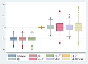
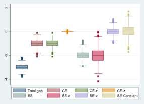
approach overcomes identification issues, we perform Monte Carlo simulations that
compare our proposal with the classical OB decomposition (see the Technical Appendix).

Estimates suggest significant differences in the gender pay gap between salaried workers
and self-employed. The magnitude of the total gap is determined by a higher gap among
self-employed workers (63.6%). Moreover, by interacting worker’s type and industry to
explain the gap, it is obtained that the gender employment share plays a mixed role. It
reduces the gap for salaried workers and expands the gap for self-employed. Overall, the
difference in the characteristics’ premia is the primary driver of the gender gap. Hence,
dropping this component, we would observe a pay gap of 4% in favor of women for
salaried workers, and a remarkably lower gap of 27.25% for self-employed.

The heterogeneity across industries is also a significant source of earning differences.
Eliminating the differences due to the population composition across industries, i.e.
assuming that men and women have the same socioeconomic characteristics over all
industries, the pay gap would decrease for salaried workers. But, it would increase for
self-employed, implying that sorting into industries contributes to reduce the gap for the
latter. This means that the flexibility provided by self-employment has a considerable cost
in terms of the pay gap, which is partially vanished by the heterogeneity in workers’
composition in socioeconomic characteristics. In the case of salaried workers, these
heterogeneities play a minor role. In sum, these findings provide insights to the
policymaking discussion regarding more flexible arrangements, vocational programs, and
care economy policies as strategies to reduce the gender gap.

The rest of the article is organized as follows. Section 2 presents an overview of the
related literature. Section 3 describes the data and presents the general context of gender
gaps by industry and type of worker. Section 4 introduces the OB decomposition type and
offers the proposed decomposition method. Section 5 discusses the main results, while
Section 6 considers some concluding remarks.

 4

2. RELATED LITERATURE

This article relates to the literature on gender sorting into type of workers and industries.
Regarding the first thread, sorting into worker’s type has been explained because of
differences in preferences to perform activities at work, comparative advantages
concerning the occupation or the jobs amenities (e.g., flexibility in working hours), and that
individuals’ value differently (Baker & Cornelson, 2018; Blau et al., 2013; Cortes & Pan,
2018; Das & Kotikula, 2019; Gallen et al., 2019; Goldin, 2014). For instance, Goldin (2014)
argues that the fact that men are employed in higher-paying industries, where women
continue to be underrepresented, is a crucial driver of the gender gap. This is consistent
with the idea that firms prefer workers that supply full-time rather than human capital, so
women pay a sort of flexibility penalty because their higher preferences for flexibility result
in working comparatively fewer hours (Bardasi & Gornick, 2008; Mumford & Smith, 2008;
Nwaka et al., 2016; Nightingale, 2019).

Although some studies have documented that self-employment might become an
alternative to reduce the pay gap, it is still present given that women tend to value more
flexible arrangements that facilitate balancing family-work responsibilities (Budig, 2006;
Craig et al., 2012; Leung, 2006; Leuze & Strauß, 2016). Mumford & Smith (2008) and
Gallen et al. (2019) present evidence on women sorting into lower-hours workplaces,
while Clain (2000), Hundley (2001), and Walker (2009) report results consistent with the
presence of strong sorting into worker’s type by comparing socioeconomic characteristics
of self-employed women and men. In the case of Latin American countries, Atal et al.
(2010) found that worker’s type plays an influential role in the unexplained gap. This
means that the gender gap is higher among self-employment, mainly driven by hours
worked and family background (see Eastough & Miller, 2004; Lechmann & Schnabel,
2012). Hence, the reasons why workers choose to be self-employed are rather diverse.
Workers might decide rationally to work as self-employed according to their abilities and
capacities to generate income. In contrast, they can be forced since the salaried workers’
sector is rationed, and it does not provide enough alternatives. These two factors, which
can be names exit and exclusion, are the leading causes of informality in developing
countries (Perry et al., 2007).

 5

Regarding the influence of industry on the gender gap, two factors can be discussed. First,
the gender composition varies between industries, so a pay gap is observed even if there
are no gender differences within industries. Secondly, industries also might pay differently
by gender, not only because of discrimination but also because of the segregation in
particular tasks. Regarding these possible sources of earnings differentials, Hodson &
England (1986), Fields & Wolff (1995), and Gannon et al. (2007) provide estimates of the
contribution of industry to the gender gap by using counterfactual decomposition
techniques. Results indicate that both components are quantitatively important since
together explain up to one-third of the total gap. Allen & Sanders (2002) address this
question and find that the social services, commerce and hotels, and business services
industries are typical female-dominated jobs. Importantly, this quantitative approach
suffers from an identification problem that appears as a consequence of choosing a
reference category, which generates interpretation issues of the decomposition results.
This problem has been primarily discussed in the study of inter-industry gender wage
differentials (see Haisken-DeNew & Schmidt, 1997; Lin, 2007; Reilly & Zanchi, 2003; Yun,
2006), where the conventional practice is to normalize the categories or to impose
coefficient restrictions.

 3. DATA AND DESCRIPTIVE STATISTICS
Using the Colombian household survey, named the Great Integrated Household Survey
(GEIH for its acronym in Spanish) for 2019, we estimate gender pay gap measures. GEIH
is a monthly-based nationwide survey that provides information about labor conditions,
family structure, and household income. The analysis was focused on the urban labor
market, considering workers located in 13 main metropolitan areas2. This was equivalent
to 150,977 observations, representing a weighted sample of 9’762,372 employees3, half
of the total employment in Colombia. 60.4% of individuals were salaried workers in this
sample, and 39.6% were self-employed.

2 Colombia has a highly segmented labor market. We focus our analysis on the urban labor market since
there are deep differences with respect to the rural labor market. In the latter, the informality rate reaches
90%, and searching, hiring and job seasonality processes have a different dynamic.
3 This results from applying the survey sampling weights.

 6

Descriptive analysis revealed essential differences in the labor market outcomes by
gender. Regarding labor income (see Table 1), the average men’s earnings were 1.46
million Colombian currency (around 450 USD4), 13.9% higher than women’s. The gap is
remarkably different by worker type, 31.7% for self-employed and 5.5% for salaried
workers. Table 1 also presents other statistics on the labor earnings distribution that show
how the gender gap varied over earning distribution. For instance, the gender gap in the
median was 7.0%, which decreased over earnings distribution from 59.3% in the 10%
quantile to 0.3% in the quantile 90%. Interestingly, the gap in hourly income was also
close to zero, which indicates that the number of hours is a relevant component of the
gender gap.

 Table 1. Descriptive statistics of the gender pay gap

 Variables Total Men Women Gap
 Average 1,362.78 1,452.20 1,250.10 13.9%
 Median 945.00 1,002.51 932.06 7.0%
 Quantile 10% 270.97 405.31 165.09 59.3%
 Quantile 90% 2,520.89 2,526.53 2,518.68 0.3%
 Standard deviation 607.93 892.98 782.90 12.3%
 Hourly average 8.43 8.45 8.41 0.5%
Source: GEIH 2019. Own calculations. Earnings values expressed in thousand Colombian pesos

There were also patterns of gender gap related to the worker’s type, as shown in the
kernel densities in Figure 1. This is consistent with the fact that women have higher
participation among low-paid self-employed (see Table 2). In the bottom 25% less paid
self-employed, women account for 67.4% of the total workers, while in the top 25% of the
same group, the participation was 35.2%. Table 2 also shows that the share of men and
women was more stable across the distribution of labor income of salaried workers.

To examine how industry relates to the gender gap, workers were classified into seven
groups of industries5: Manufacturing (including services and utilities); Construction;
Commerce; Transport and communication; Professional services6; Public administration7

4 To have some reference, exchange rate in 2019 was 3,277.14 Colombian pesos as for December 31st.
5 Agriculture, and mines and quarries, were not included in this analysis given their low representativeness
in urban areas.
6 The industry is composed by professional and scientific activities, finance activities and real estate

activities.
7 The industry is composed by public and defense administration, education, services for the health.

 7

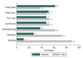
and Other services (including entertainment, artistic, recreation, and similar activities).
Estimating the industry size in terms of employment, it was observed that Manufacturing
and Commerce provided almost half of the total employment (29.1% and 15.9%,
respectively), while the individual contribution of the rest of the industries was below 15%.
Industries also differed in the composition between salaried workers and self-employed.
For instance, Commerce had the most significant proportion of workers in both cases.
Nonetheless, the percentage of self-employment in Other services and Transport and
communication was above that for salaried workers. On the other hand, Construction
exhibited low participation of workers in both cases.

 Figure 1. Earnings distribution by job type

 a. Salaried workers b. Self-employed

Source: GEIH 2019. Own calculations.

 Table 2. Gender share across earnings distribution by type of worker

 Salaried workers Self-employed
 Variables
 Total Bottom 25% Top 25% Total Bottom 25% Top 25%
 Women 43.70% 48.2% 44.3% 44.4% 67.4% 35.2%
 Men 56.30% 51.8% 55.7% 55.6% 32.6% 64.8%
 Difference 12.6% 3.6% 11.5% 11.2% -34.8% 29.6%
Source: GEIH 2019. Own calculations. Each value corresponds to the percentage of men or women in a
particular quartile of the earnings distribution.

Gender composition within industries was also quite dissimilar (see Figure 2). Among
salaried workers, all industries were male-dominated except for Public Administration and

 8

Other services, where women were 62.0% and 51.2%, respectively. For the rest of the
industries, it was remarkable that Construction (88.8%) and Transport and communication
(72.9%) were male-dominated. In the case of self-employed, the composition was more
balanced; women were more represented in three sectors: Public Administration;
Professional Services; and Other services. In turn, the proportion of men was more
pronounced in Construction (97.7%) and Transport and communication (93.3%). Overall,
this is strong evidence of the sorting into industry and type of worker.

 Figure 2. Employment distribution across industries and worker types

 a. Salaried workers b. Self-employed

Source: GEIH 2019. Own calculation.

To summarize how the gender gap is affected by industry and worker’s type, the raw labor
earnings difference across these characteristics was computed. Figure 3 implies that the
gender gap had a high variation, although lower for salaried workers. Indeed, the higher
gap for this group was 23.0% in Public Administration, while among self-employed, the
higher gap was 55.0% in Professional services. In addition, Construction was the only
industry with a negative gap, although it was also the industry with the lowest female
participation. Transport, a male-dominated industry, had a negative gap for salaried
workers and was the second lowest among the self-employed. In short, it was observed
that industries with high participation of women employees had a higher gender gap.

 9

Figure 3. Pay gap by industry and worker type

 a. Salaried workers

 3,000 30.0
 23.0
 2,500 20.0
 14.3 17.0
 9.4 10.0
 2,000 6.5
 Earnings

 -2.6 -
 1,500
 -10.0
 1,000
 -20.0
 500 -30.0
 -33.4
 - -40.0

 Women Men Gap (%)

 b. Self-employed

 3,000 80.0
 55.0
 2,500 44.3 44.5 40.0
 33.0 38.7
 Earnings

 2,000 8.9
 0.0
 1,500
 -40.0
 1,000
 500 -83.5 -80.0

 0 -120.0

 Women Men Gap (%)

Source: GEIH 2019. Own calculations. Left axes measure the earnings in thousand Colombian pesos and
right axes the gender gap in %.

Analyzing additional workplace features, it was revealed that for most industries, salaried
workers men tended to report more working hours, and were in larger firms8. In turn, men’s
informality rate9 was higher, especially in industries with lower women’s employment

8 Firm’s size is defined as follows: small firms are firms with five workers or less, medium firms are firms
between 6 and 50 workers, and large firms are firms with more than 50 workers.
9 Informality is defined as workers who are not affiliated to health or neither contribute to a pension nor are

pensioners.

 10

participation (see Table 3). Gender differences in these characteristics were more
 significant among self-employed. For instance, there was a gap in working hours which
 was more pronounced for self-employed. While salaried workers reported more working
 hours on average than self-employed workers, the gender gap in this item was higher for
 the self-employed. Accordingly, the gender gap in working hours was 17 hours for salaried
 workers and 48 hours for self-employed. Thus, women were sorting into jobs with lower
 working hours. Women in Public Administration were the group of salaried workers with
 fewer working hours, 169 on average. In all other industries, self-employed women
 worked significantly fewer hours. Besides, different expected results were that self-
 employed were informal and worked in small firms.

 Table 3. Workplace characteristics for salaried workers and self-employed

 Manufacturing Construction Commerce Transport Prof. Serv. Public adm Other serv.
Variables
 Women Men Women Men Women Men Women Men Women Men Women Men Women Men
Salaried Workers
All 38.0 62.0 11.2 88.8 47.6 52.4 27.1 72.9 47.7 52.3 62.0 38.0 51.2 48.8
Informality
Yes 26.1 20.7 14.3 35.7 44.9 39.1 15.9 15.3 9.8 10.7 8.8 5.6 35.9 34.6
Hours worked
mean 184.5 192.9 178.4 192.3 185.1 199.6 180.0 204.3 174.6 193.7 169.0 189.0 175.7 181.6
Size of firm
Small 14.3 12.5 7.3 27.0 37.4 30.7 12.7 14.4 11.3 14.3 4.2 1.2 22.9 21.9
Medium 31.6 29.4 34.9 36.7 32.9 36.5 18.7 18.9 23.9 30.6 18.3 9.6 33.8 32.1
Large 54.1 58.1 57.8 36.4 29.7 32.8 68.7 66.7 64.8 55.2 77.5 89.2 43.4 46.0

Self-employed workers
All 49.5 50.5 2.3 97.7 50.7 49.3 6.7 93.3 61.0 39.0 65.6 34.4 55.2 44.8
Informality
Yes 92.3 88.2 57.8 91.3 93.9 90.9 76.1 77.9 79.1 69.4 43.5 26.9 91.3 88.6
Hours worked
mean 147.4 185.3 138.4 166.7 145.7 199.5 175.3 221.0 128.5 162.2 148.8 151.1 128.1 165.8
Size of firm
Small 87.7 84.9 45.1 95.9 97.7 94.5 80.7 93.9 90.6 89.2 45.2 25.4 89.9 90.6
Medium 9.8 10.0 32.5 3.1 1.8 4.7 6.3 2.6 5.5 6.4 8.9 8.8 5.8 5.9
Large 2.5 5.1 22.5 1.1 0.5 0.8 12.9 3.5 3.9 4.4 45.9 65.8 4.3 3.6
 Source: GEIH 2019. Own calculations. Working hours correspond to the monthly-equivalent average.
 4

 11

Table 4 shows that there were also differences in the socioeconomic composition of
 employment. Women were higher educated than men, especially in the Construction
 industry. It was also noticeable that, on average, salaried workers had more years of
 education than self-employed. In addition, in most cases, the proportion of household
 head women was higher for self-employed. This was also true for married women. These
 two facts were consistent with the findings regarding women's motivation to work as self-
 employed since these jobs facilitate the family-work balance.
 Table 4. Socioeconomic characteristics for salaried workers and self-employed

 Manufacturing Construction Commerce Transport Prof. serv. Public adm Other serv.
Variables
 Women Men Women Men Women Men Women Men Women Men Women Men Women Men
Salaried workers
% 38.0 62.0 11.2 88.8 47.6 52.4 27.1 72.9 47.7 52.3 62.0 38.0 51.2 48.8
Age
Average 36.6 36.7 34.3 36.8 34.1 33.9 33.9 37.5 33.9 36.3 38.7 39.5 35.2 35.3
Education
Average
 11.7 11.1 13.4 9.2 11.3 10.9 13.6 11.7 13.5 12.5 14.5 14.4 12.4 12.1
years
Marital status
% with
 47.2 59.6 49.4 62.8 46.5 51.8 43.9 60.0 44.6 54.8 51.5 60.6 43.3 50.7
partner
Household head
Yes 33.1 53.1 31.1 55.2 32.3 47.2 26.8 57.4 30.6 53.6 35.0 62.1 32.6 49.4
Self-employed
% 49.5 50.5 2.3 97.7 50.7 49.3 6.7 93.3 61.0 39.0 65.6 34.4 52.8 47.2
Age
Average 45.9 45.0 39.0 45.2 44.5 44.5 40.7 42.7 43.9 45.9 39.3 38.7 41.6 41.4
Education
Average
 9.4 9.0 13.2 8.1 9.2 8.7 11.5 9.3 10.4 13.7 13.6 15.5 10.1 10.4
years
Marital status
% with
 55.7 64.1 35.2 63.6 56.1 62.9 50.8 63.8 44.9 56.7 51.5 50.1 49.7 47.9
partner
Household head
Yes 37.8 63.7 27.4 57.9 40.4 61.5 34.7 57.5 45.3 64.9 31.8 51.1 37.9 53.1
 Source: GEIH 2019. Own calculations.

 4. DECOMPOSITION METHOD
 4.1 OAXACA-BLINDER DECOMPOSITION
 Counterfactual decomposition methods are the most popular technique to investigate the
 sources of gender pay gaps. This method consists of computing two components known
 as composition effect [CE] and structure effect [SE]. The first is the part of the earnings

 12

gap due to the differences in the population composition, also known as an explained
effect. The second is the remainder which is interpreted as a structure effect (or
unexplained component). Implementing these methods requires specifying the relation
between labor earnings and workers’ characteristics estimated using regression
techniques (see Chernozhukov et al. (2013), for a broad discussion)10.

The starting point is the total average difference of labor earnings, ∆ , defined as follows:
 ∆ = − 
Where and are the average earnings of men and women. Oaxaca (1973) and
Blinder (1973) propose to write this difference as follows:
 
 ∆ = ′ ′ ′ ′ ′ 
 − = ( − ) + ( − ) (1)
The first term on the right-hand side corresponds to the composition effect (CE), while the
second corresponds to the structure effect (SE) as it depends on the gender specific
 
earnings structure11. Note that ′ refers to the vector of the average of the observed
characteristics for the group , and "′" denotes transpose.

Previous work studying the quantitative importance of industry on the gender gap has
included gender employment shares by industry and dummies at the industry level as
regressors. The individual contribution of each factor is estimated as the sum of the CE
and the SE depending by these variables (see Fields & Wolff, 1995; Gannon et al., 2007).
Jones (1983) and Oaxaca & Ransom (1999) have pointed out that this approach suffers
from the so-called omitted group identification issue, which is related to the sensitivity of
the choice of the reference category as the coefficient of that industry is not distinguishable
from the constant term. Alternative solutions to the problem can be found in Oaxaca &
Ransom (1999), Horrace & Oaxaca (2001), and Yun (2005). These solutions consist of
normalizing the regressor, imposing a restriction on the coefficients, or netting out the
effect of the omitted group contained in the constant terms.

10 This approach provides an aggregated decomposition for the difference the average pay, but it can be
extended in order to assess the quantitative relevance of workers characteristics individually or studying
the difference in other functionals of the labor earnings distribution (Machado & Mata, 2005; Melly, 2005;
Rothe, 2010).
 
11
 The term ′ is a counterfactual outcome representing the average earnings that men would obtain if
they had same characteristics than women, which is not observable.

 13

4.2 A TWO-STEP DECOMPOSITION METHOD
An alternative decomposition method is proposed based on a two-step procedure to
overcome the possible identification and interpretability issues. The first step consists of
estimating the contribution of the gender employment shares by industry, while the second
implements OB decompositions to quantify the importance of the earnings schedule at
the industry level.

In the first step, the average of labor earnings is expressed as a weighted average of the
industry labor earnings, that is

 ∆ = − = ∑ ( − )
 =1

where represents men’s share of employment in the industry , is the corresponding
average earnings, and the total number of industries. Re-arranging terms, the total
difference can be written as:
 
 ∆ = ∑ ( − ) + ∑ ( − ) . (2)
 =1 =1

The first term captures the part of the gender gap due to the difference in average
earnings, while the second measures the component on behalf of differences in
employment shares.

To explore the part of the gender gap related to the idiosyncratic industry’s pay structure,
the terms − are decomposed using OB decompositions. In such a way, using
Equation (1) into Equation (2), the final decomposition is given by:

 ∆ = ∑ ( ′ − ′ ) + ∑ ′ ( − )
 =1 =1
 
 +∑ ( − ) (3)
 =1

where the first term is an aggregated composition effect (ACE), which is computed as the
weighted average of the CE at the industry level. The second is related to the industries’
earnings structure, named aggregated structure effect (ASE), and the third is the
employment-share effect (ESE).

 14

This decomposition allows to directly quantify the importance of gender employment
allocation avoiding the omitted group issue. Besides, the heterogeneity in the returns of
 
workers’ characteristics, that is captured by variation in ′ ( − ), reflects the

differences in the production technology, and others industry features shaping the pay
 
schedule. Similarly, the variability of ( ′ − ′ ) across industries makes it

possible to study the contribution of the sorting in employment composition on the pay
gap. This decomposition is essentially based on exploiting the conditional distributions
instead of the joint distribution in order to obtain more detailed components that allow to
identify the nature of the gap.

Considering these three components, it is possible to build counterfactuals related to the
contribution of industry to the total gap. For instance, to measure the gap assuming that
any of the components are zero, which means dropping composition or returns differences
between men and women. And secondly, to assess how the gap change when the
heterogeneity between industries is eliminated, i.e., assuming that composition and
structure effect behaves as the average12. From this decomposition, some quantities of
interest can be studied. For instance, the sum of ACE and ESE would be the observed
gender gap in the absence of gender and industry differences in premia, i.e., if industries
equally pay for men and women’s characteristics. The sum of the terms ACE and ASE
quantifies the gender gap that one would observe if men and women workers in the same
proportion in each industry, which is the total effect due to the variation in the average
income (say, Total Pay Effect, TPE).

 5. THE CONTRIBUTION OF INDUSTRY AND TYPE OF WORKER TO GENDER GAPS
Based on raw estimation of the pay gap, we observe that the gender gap varied
significantly across worker’s type, i.e., while the gender gap among salaried workers was
4.2%, the estimate among self-employed was 63.63%13. Using the proposed method,

12 In the technical appendix, it is provided a detailed description of the method and some simulation
results showing how the method performed in comparison to the OB decomposition.
13
 This value differ from the previous analysis since the decomposition is performed on the logarithm of the
earnings to facilitate the implementation and interpretation.

 15

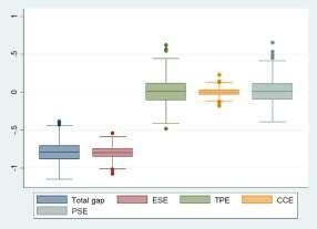
decomposition analysis for salaried workers and self-employed, separately, was
performed. First, the contribution of the gender employment shares and average pay gap
at the industry level was estimated on the total gender gap. Subsequently, the latter
component was decomposed into composition and structure effects.

The specification used for the decomposition includes the following controls: age,
education, marital status, whether the individual is a household head, number of working
hours (in logs), firm size, informality status, and job qualification (job position as
professional or director). Confidence intervals at 95% were computed using 1,000
bootstrapping simulations. Results for the aggregate decomposition show that the gender
gap was explained mainly by the differences in average pay across industries (see Table
5). In turn, the share effect was negative and statistically significant, but it was not
quantitatively relevant. This indicates that female and male employment allocation across
industries tends to narrow the gap slightly. In fact, based on the two components
estimates, a gap of 1.4% in favor of women would be observed if all industries would pay
equally men and women.

For self-employed, results were remarkably different. The pay effect was still the main
driver; however, the ESE was positive and had a significant contribution, 11.7 percentage
points equivalent to 18.3% of the total gap. This might be related to gender sorting into
industries for self-employed, which, in this case, is consistent with the lower labor income
in industries such as retail and services.

 Table 5. Aggregate decomposition by worker type

 Salaried workers Self-employed
 0.042 0.636
 Total gap
 [0.033 , 0.051] [0.623 , 0.656]
 0.056 0.519
 TPE
 [0.045 , 0.065] [0.478 , 0.561]
 -0.014 0.117
 ESE
 [-0.019 , -0.007] [0.084 , 0.157]
Source: Own calculations. 95% confidence interval is brackets estimated using 1000 bootstrapping
simulations. TPE is the total pay gap and ESE is the employment share effect.

 16

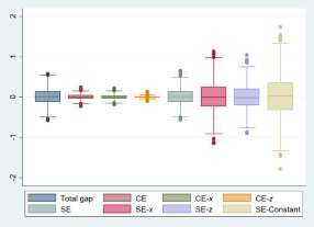
An important question arising here is how much gender differences in workers'
characteristics or gender differences in the returns account for the pay effect. To answer
this, the second step of the decomposition is estimated. Figure 4 presents the point
estimates and 95% confidence intervals for the ACE and ASE. Although the TPE was
positive for salaried workers, the part of the gap that depends on the characteristics of the
workers had a negative sign. In this scenario, if the characteristics were paid the same
within industries, a pay gap of 4% (ESE+ACE) in favor of women would be observed. This
is a significant result, as it highlights that the premium differential is the main driver of the
gender gap for salaried workers. Noticeably, the gap prevailed even when controlling for
the number of hours worked, informality status, and job qualification.

 Figure 4. Two-step decomposition by worker type.

 a. Salaried workers

 0.12

 0.08

 0.04

 0.00

 -0.04

 -0.08
 Total TPE ACE ASE ESE

 b. Self-employed

 0.70
 0.60
 0.50
 0.40
 0.30
 0.20
 0.10
 0.00
 Total TPE ACE ASE ESE

Source: Own calculations. 95% confidence interval is brackets estimated using 1000 bootstrapping
simulations. TPE is the total pay gap, ACE is the aggregated composition effect, ASE is the aggregated
structure effect, and ESE is the employment share effect.

 17

The ASE was also the main component of the TPE for the self-employed, but in contrast,
the composition effect was positive. This result is aligned with Goldin (2014), who argues
that women are self-selected into jobs where flexibility is a key factor in the labor supply
decision. In sum, these decomposition exercises show that even if the participation of
women and men in the industries were the same, and that men and women within each
industry had the same characteristics, a gap of 8.2% and 36.38% (i.e., the ASE) would be
observed between salaried workers and self-employed workers, respectively. That is, the
remainder, i.e., the sum between ACE and ESE, was negative for salaried workers,
implying that these factors reduced the gap. In contrast, in the case of the self-employed,
both factors expanded the pay gap, accounting for around 40% of the total gap.

One of the advantages of the proposed decomposition method is that it allows quantifying
the contribution to the gender gap components at the industry level. Figure 5 presents the
percentage of this contribution measured as the corresponding elements of the
summation in Equation (3). Two facts are evident. First, individual contributions at the
industry level were not equal, implying that industries’ features shape the composition and
structure effect. Second, ASE was positive for all industries for both worker types, showing
systematic, higher premia for men.

An expected result was that industries with the most significant gender share difference
and pay gender gaps exhibited more substantial influence on the components. In
particular, for salaried workers, Construction had the higher contribution to the ACE, which
was in favor of women, but at the same time, everything being equal generated a higher
gap in terms of characteristics’ premia. Moreover, Public administration, a female-
dominated industry, also positively contributed to the ASE. The mixed results across
industries revealed by the ACE also show strong gender sorting patterns. Among the self-
employed, the ACE and the ASE were determined by industries such as Transportation,
Construction, and Commerce. The first two correspond to male-dominated industries,
while the latter was a sector with a similar gender employment share but with the most
significant pay gap.

 18

Figure 5. Industry contribution to the decomposition components.

 a. Salaried workers
 100%
 80%
 60%
 40%
 20%
 0%
 -20%
 -40%
 -60%
 -80%
 ESE ACE ASE Total
 Manufacturing Building Commerce Transp and comm
 Prof. services Public admin Other services

 b. Self-employed
 100%
 80%
 60%
 40%
 20%
 0%
 -20%
 -40%
 -60%
 ESE ACE ASE Total
 Manufacturing Building Commerce Transp and comm
 Prof. services Public admin Other services

Source: Own calculations. ACE is the aggregated composition effect, ASE is the aggregated structure effect,
and ESE is the employment share effect.

Finally, the role of heterogeneity across industries by performing industry-level
decompositions was explored. Figure 6 and Figure 7 present the CE and SE in a
disaggregated manner for each characteristic. In terms of the CE, education played a
crucial role in reducing the gender gap for both worker types in terms of the CE. From the
perspective of employment characteristics, factors such as working hours and job
qualification were essential forces leading to a positive gap in the case of self-

 19

employment. Regarding working hours, the CE is positive in all industries, consistent with
the fact that women choose jobs that allow them to balance work and personal life.

Figure 6. Industry contribution to decomposition components for gender gap for salaried
 workers.

 a. Composition effect

 Informal

 Qualified job

 Large firm

 Med. Form

 Wk hours

 Married

 HH head

 Education

 Age

 -0.40 -0.35 -0.30 -0.25 -0.20 -0.15 -0.10 -0.05 0.00 0.05 0.10 0.15
 Other services Public adm Prof. services Transport and comm
 Commerce Building Manufacturing

 b. Structure effect

 Informal

 Qualified job

 Large firm

 Med. Form

 Wk hours

 Married

 HH head

 Education

 Age

 -2.00 -1.50 -1.00 -0.50 0.00 0.50 1.00 1.50 2.00
 Manufacturing Building Commerce Transport and comm
 Prof. services Public adm Other services
Source: Own calculations.

 20

Figure 7. Industry contribution to decomposition components for gender gap for self-
 employed.

 a. Composition effect

 Informal

 Qualified job

 Large firm

 Med. Form

 Wk hours

 Married

 HH head

 Education

 Age

 -0.30 -0.20 -0.10 0.00 0.10 0.20 0.30 0.40
 Manufacturing Building Commerce Transport and comm
 Prof. services Public adm Other services

 b. Structure effect

 Informal

 Qualified job

 Large firm

 Med. Form

 Wk hours

 Married

 HH head

 Education

 Age

 -1.00 -0.80 -0.60 -0.40 -0.20 0.00 0.20 0.40 0.60 0.80 1.00
 Manufacturing Building Commerce Transport and comm
 Prof. services Public adm Other services
Source: Own calculations.

The analysis of the SE shows a higher contribution of education and working hours. This
draws attention to two key issues. There is additional evidence of the relevance of
flexibility as a factor driving self-selection since, even when the return per marginal hour

 21

was higher for women, this group chose to work fewer hours. An additional result was that
the informality premium played an important role among self-employed. In fact, this factor
tended to increase the gender gap, i.e., an informal male self-employed earned much
more than a female counterpart.

To get an overview of the results, the relationship between the level of feminization of the
industries14 with the magnitude of decomposition components was studied (see Figure 8).
The higher the feminization, the lower the employment share effect. In contrast, ACE had
a positive relationship with feminization, while for ASE, is negative, although the latter is
a weaker relationship. This shows that the most feminized industries, which coincide with
labor-intensive activities, and possibly industries with lower productivity, contribute more
to enlarge the gender gap.

 Figure 8. Industry feminization and decomposition components

 a. Salaried workers b. Self-employed
 ESE ESE
 3.0 4.0

 2.0 3.0

 1.0 2.0
 ESE

 ESE

 0.0 1.0
 0 20 40 60 80
 -1.0 0.0
 0 20 40 60 80
 -2.0 -1.0

 -3.0 -2.0
 % women in the industry % women in the industry

 ACE ACE

14
 Level of feminization is a measure of the proportion of female employees over total employees in an
industry. The higher proportion the high feminization.

 22

0.04 0.12

 0.02 0.09

 0.06
 0.00
 0 20 40 60 80 0.03
 ACE

 ACE
 -0.02
 0.00
 -0.04 0 20 40 60 80
 -0.03
 -0.06 -0.06

 -0.08 -0.09
 % women in the industry % women in the industry

 ASE ASE
 0.03 0.18

 0.02 0.15

 0.12
 0.02
 ASE

 ASE
 0.09
 0.01
 0.06
 0.01 0.03

 0.00 0.00
 0 20 40 60 80 0 20 40 60 80
 % women in the industry % women in the industry

Source: Own calculations.

Overall, results suggest that heterogeneity across industries is crucial to understanding
the sources of gender gaps. Using the above estimates, it was possible to perform
counterfactual exercises to obtain additional evidence about the role of industry
heterogeneity. In particular, it is possible to assess how the gender gap would change in
scenarios where variability in either gender employment shares, population composition
within industries or premia is eliminated. For this, the components of Equation (3) were
estimated under three assumptions: i. the proportion of men and women is equal in all
industries, ii. the CE of each industry is equivalent to the labor market average, and iii. the
SE of each industry is equivalent to the labor market average.

 23

These scenarios were compared to determine whether the variation between industries
contributes to increasing or decreasing the gap15. The results in Table 6 indicated that if
all industries have a 50-50 gender composition, the gender gap would increase for
salaried workers but reduce for self-employed. This implies that the higher participation of
women in male-dominated industries does not necessarily reduce the pay gap. These
mixed results were also found when the CE heterogeneity was dropped. On the one hand,
CE heterogeneity increases the gap between salaried workers. Without such variability,
the gap would decrease by 0.9 percentage points.

On the other hand, the gap among the self-employed would increase by 14.2 percentage
points. Finally, the heterogeneity in the SE provoked the smallest change concerning the
estimated gap for both worker types. Consequently, these findings support the idea that
industry affects the gender gap mainly through gender share and employed composition.
Besides, a substantial improvement was observed for self-employed since employment
shares at the industry level contribute with 14.6 percentage points, 23% of the total gap.

 Table 6. Gender gap and components heterogeneity between industries

 Salaried workers
 Benchmark Equal shares Equal ACE Equal ASE
 Total gap 0.042 0.049 0.033 0.037
 TPE 0.056 0.049 0.047 0.050
 ACE -0.026 -0.038 -0.035 -0.026
 ASE 0.082 0.087 0.082 0.077
 ESE -0.014 0.000 -0.014 -0.014
 Self-employed
 Benchmark Equal shares Equal ACE Equal ASE
 Total gap 0.636 0.490 0.778 0.612
 TPE 0.519 0.490 0.661 0.494
 ACE 0.155 0.215 0.297 0.155
 ASE 0.364 0.275 0.364 0.339
 ESE 0.117 0.000 0.117 0.117
Source: Own calculations. TPE is the total pay gap, ACE is the aggregated composition effect, ASE is the
aggregated structure effect, and ESE is the employment share effect.

15
 Of course, this exercise does not take into account general equilibrium effects, since it is assuming
independence among the components, i.e., it is assumed that equalizing the premia across industries would
not generate variations in gender composition or worker characteristics. However, these exercises can be
informative about the sources of pay inequality between men and women.

 24

6. CONCLUDING REMARKS

Reducing the gender pay gap is perhaps one of the most urgent issues to improve
inclusiveness in the labor market. Policymakers have focused on designing policies
reducing discrimination and most recently, on promoting programs that facilitate women’s
access to better jobs. These policies have been motivated by the evidence of gender
sorting into worker’s type and industries, another factor contributing to the gender pay
gaps. This article documents the relevance of this sorting as a force driving the gender
gap in Colombia. Notably, evidence is provided that gender employment shares and
heterogeneity in workers’ population and characteristics’ returns affect the earning
differences.

A higher proportion of men or women in a particular industry has been an indicator of
segregation. This factor is crucial to understanding the sources of the gender gap. Our
estimates show that industries with high participation of women have the highest gender
pay gap, and this pattern is strong among self-employed. However, it is also obtained that
a more equalized distribution of men and women across sectors would result in a lower
pay gap for this group. What is behind is that men and women consider preferences for
occupations, flexibility, and comparative advantages for job search decisions. This means
that anti-discrimination regulations might not be enough to reduce gender gaps (see c.f.
Morton et al., 2014). On the contrary, other elements also determine the gap through the
occupational choice decision.

As discussed by Clain (2000), Goldin (2014), and Eastough & Miller (2004), the higher
gender pay gap among self-employed not only combines wage discrimination and
premium gaps but also relates to temporal flexibility and unpaid work. Even tax and
subsidy structures might play a role in determining gender equality (see c.f. Duval-
Hernandez et al., 2021). In this way, promoting women’s employment in male-dominated
industries is a relevant strategy to reduce the job access gap. Still, in the light of our
results, it might not turn out to reduce the gender pay gaps. Therefore, a policy design
must target the reduction of segregation into high value-added sectors, which requires
programs related to forming aspiration and flexible arrangements (see Das & Kotikula,
2019, for further discussions).

 25

DECLARATIONS

Ethical Approval: Not applicable

Competing Interests Statement: The authors of this research certify that they have no
conflict of interests in this manuscript.

Authors' contributions: Both authors have equally contributed to write the main
manuscript text and data process which includes cleaning, coding and results analysis.

Funding: Andres Garcia-Suaza thanks the support of Alianza EFI-Colombia Científica
grant with code 60185 and contract number FP44842-220-2018, funded by The World
Bank through the call Scientific Ecosystems, managed by the Colombian Ministry of
Science, Technology and Innovation.

Availability of data and materials: All data used in this paper are publicly available on
the DANE (Colombian, National Statistical Institute) website. Processing details and
replication codes are available upon request.

 26

REFERENCES
Allen, J., & Sanders, K. (2002). Gender gap in earnings at the industry level. European
Journal of Women's Studies, 9(2), 163-180.
Altonji, J. G., & Blank, R. M. (1999). Race and gender in the labor market. Handbook of
labor economics, 3, 3143-3259.
Atal, J. P., Ñopo, H., & Winder, N. (2010). Gender and Ethnic Wage gaps in Latin
America at the turn of the Century. Inter-American Development Bank.
Baker, M., & Cornelson, K. (2018). Gender-based occupational segregation and sex
differences in sensory, motor, and spatial aptitudes. Demography, 55(5), 1749-1775.
Bardasi, E., & Gornick, J. C. (2008). Working for less? Women's part-time wage penalties
across countries. Feminist economics, 14(1), 37-72.
Blau, F. D., & Kahn, L. M. (1997). Swimming upstream: Trends in the gender wage
differential in the 1980s. Journal of labor Economics, 15(1, Part 1), 1-42.
Blau, F. D., Brummund, P., & Liu, A. Y. H. (2013). Trends in occupational segregation by
gender 1970–2009: Adjusting for the impact of changes in the occupational coding
system. Demography, 50(2), 471-492.
Blau, F. D., & Kahn, L. M. (2017). The gender wage gap: Extent, trends, and
explanations. Journal of economic literature, 55(3), 789-865.
Blinder, A. S. (1973). Wage discrimination: reduced form and structural estimates. Journal
of Human resources, 436-455.
Budig, M. J. (2006). Gender, self-employment, and earnings: The interlocking structures
of family and professional status. Gender & society, 20(6), 725-753.
Clain, S. H. (2000). Gender differences in full-time self-employment. Journal of Economics
and Business, 52(6), 499-513.

Chernozhukov, V., Fernández‐Val, I., & Melly, B. (2013). Inference on counterfactual
distributions. Econometrica, 81(6), 2205-2268.
Cortes, P., & Pan, J. (2018). Occupation and gender. The Oxford handbook of women
and the economy, 425-452.
Craig, L., Powell, A., & Cortis, N. (2012). Self-employment, work-family time and the
gender division of labour. Work, employment and society, 26(5), 716-734.
Das, S., & Kotikula, A. (2019). Gender-based employment segregation: Understanding
causes and policy interventions. World Bank.

 27

Duval-Hernandez, R., Fang, L., & Ngai, R. (2021). Taxes, Subsidies, and Gender Gaps
in Hours and Wages.

Eastough, K., & Miller, P. W. (2004). The gender wage gap in paid‐and self‐employment
in Australia. Australian Economic Papers, 43(3), 257-276.
Fernandez, MP. (2006). Determinantes del diferencial salarial por género en Colombia,
1997-2003. Revista Desarrollo y Sociedad, (58), 165-208.
Fields, J., & Wolff, E. N. (1995). Interindustry wage differentials and the gender wage
gap. ILR Review, 49(1), 105-120.
Fortin, N., Lemieux, T., & Firpo, S. (2011). Decomposition methods in economics.
In Handbook of labor economics (Vol. 4, pp. 1-102). Elsevier.
Gallen, Y., Lesner, R. V., & Vejlin, R. (2019). The labor market gender gap in Denmark:
Sorting out the past 30 years. Labour Economics, 56, 58-67.
Gannon, B., Plasman, R., Ryex, F., & Tojerow, I. (2007). Inter-industry wage differentials
and the gender wage gap: evidence from European countries. Economic and Social
Review, 38(1), 135.
Goldin, C. (2014). A grand gender convergence: Its last chapter. American Economic
Review, 104(4), 1091-1119.
Haisken-DeNew, J. P., & Schmidt, C. M. (1997). Interindustry and interregion differentials:
Mechanics and interpretation. Review of economics and Statistics, 79(3), 516-521.
Hodson, R., & England, P. (1986). Industrial structure and sex differences in
earnings. Industrial Relations: A Journal of Economy and Society, 25(1), 16-32.
Horrace, W. C., & Oaxaca, R. L. (2001). Inter-industry wage differentials and the gender
wage gap: An identification problem. ILR Review, 54(3), 611-618.
Hundley, G. (2001). Why women earn less than men in self-employment. Journal of labor
research, 22(4), 817-829.
ILO (2018). Global Wage Report 2018/19: What lies behind gender pay gaps.
International Labour Office.
Jann, B. (2008). The Blinder–Oaxaca decomposition for linear regression models. The
Stata Journal, 8(4), 453-479.
Jones, F. L. (1983). On decomposing the wage gap: a critical comment on Blinder's
method. The Journal of human resources, 18(1), 126-130.

 28

Lechmann, D. S., & Schnabel, C. (2012). Why is there a gender earnings gap in self-
employment? A decomposition analysis with German data. IZA Journal of European
Labor Studies, 1(1), 1-25.
Leuze, K., & Strauß, S. (2016). Why do occupations dominated by women pay less? How
‘female-typical’work tasks and working-time arrangements affect the gender wage gap
among higher education graduates. Work, employment and society, 30(5), 802-820.
Leung, D. (2006). The male/female earnings gap and female self-employment. The
Journal of Socio-Economics, 35(5), 759-779.
Lin, E. S. (2007). On the standard errors of Oaxaca-type decompositions for inter-industry
gender wage differentials. Economics Bulletin, 10(6), 1-11.
Machado, J. A., & Mata, J. (2005). Counterfactual decomposition of changes in wage
distributions using quantile regression. Journal of applied Econometrics, 20(4), 445-465.
Melly, B. (2005). Decomposition of differences in distribution using quantile
regression. Labour economics, 12(4), 577-590.
Mincer, J., & Polachek, S. (1974). Family investments in human capital: Earnings of
women. Journal of political Economy, 82(2, Part 2), S76-S108.
Morton, M., Klugman, J., Hanmer, L., & Singer, D. (2014). Gender at work: A companion
to the world development report on jobs. Washington, DC: World Bank.
Mumford, K., & Smith, P. N. (2008). What determines the part-time and gender earnings
gaps in Britain: evidence from the workplace. Oxford Economic Papers, 61, 56-75.
Nwaka, I. D., Guven-Lisaniler, F., & Tuna, G. (2016). Gender wage differences in Nigerian
self and paid employment: Do marriage and children matter?. The Economic and Labour
Relations Review, 27(4), 490-510.
Nightingale, M. (2019). Looking beyond average earnings: Why are male and female part-
time employees in the UK more likely to be low paid than their full-time
counterparts?. Work, Employment and Society, 33(1), 131-148.
Ñopo, H. (2008). Matching as a tool to decompose wage gaps. The review of economics
and statistics, 90(2), 290-299.
Oaxaca, R. (1973). Male-female wage differentials in urban labor markets. International
economic review, 693-709.
Oaxaca, R. L., & Ransom, M. R. (1999). Identification in detailed wage
decompositions. Review of Economics and Statistics, 81(1), 154-157.

 29

O'Neill, J., & Polachek, S. (1993). Why the gender gap in wages narrowed in the
1980s. Journal of Labor economics, 11(1, Part 1), 205-228.
Perry, G. (Ed.). (2007). Informality: Exit and exclusion. World Bank Publications.
Razzu, G., & Singleton, C. (2018). Segregation and gender gaps in the United Kingdom's
great recession and recovery. Feminist Economics, 24(4), 31-55.
Reilly, K. T., & Zanchi, L. (2003). Industry wage differentials: how many, big and significant
are they?. International Journal of Manpower.
Rivero, R. Y., & Mesa, C. (1997). Ingresos laborales de hombres y mujeres en Colombia:
1976-1995. Archivos de Maccroeconomía.
Rothe, C. (2010). Nonparametric estimation of distributional policy effects. Journal of
Econometrics, 155(1), 56-70.
Rothe, C. (2015). Decomposing the composition effect: the role of covariates in
determining between-group differences in economic outcomes. Journal of Business &
Economic Statistics, 33(3), 323-337.
Sin, I., Stillman, S., & Fabling, R. (2020). What Drives the Gender Wage Gap? Examining
the Roles of Sorting, Productivity Differences, Bargaining and Discrimination. The Review
of Economics and Statistics, 1-44.
Tenjo, J., & Bernat, F. (2018). Diferencias por género en el mercado laboral colombiano:
mitos y realidades. Universidad Jorge Tadeo Lozano.
Walker, J. R. (2009). Earnings, effort, and work flexibility of self-employed women and
men: the case of St. Croix County, Wisconsin. Journal of Labor Research, 30(3), 269-288.
WEF 2021. Global Gender Gap Report 2021
Yun, M. S. (2005). A simple solution to the identification problem in detailed wage
decompositions. Economic inquiry, 43(4), 766-772.
Yun, M. S. (2006). Revisiting Inter-industry wage differentials and the gender wage gap:
an identification problem.

 30