CS162 Operating Systems and Systems Programming Lecture 19 Filesystems 1: Performance (Con't), Queueing Theory, Filesystem Design - Prof. Anthony ...

CS162
 Operating Systems and
 Systems Programming
 Lecture 19

Filesystems 1: Performance (Con’t),
Queueing Theory, Filesystem Design

 April 5th, 2022
 Prof. Anthony Joseph and John Kubiatowicz
 http://cs162.eecs.Berkeley.edu

Recall: Magnetic Disks
 Track
 Sector
 • Cylinders: all the tracks under the
 head at a given point on all surfaces Head
 • Read/write data is a three-stage process: Cylinder
 – Seek time: position the head/arm over the proper track Platter

 – Rotational latency: wait for desired sector to rotate under r/w head
 – Transfer time: transfer a block of bits (sector) under r/w head

 Disk Latency = Queueing Time + Controller time +
 Seek Time + Rotation Time + Xfer Time
 Controller
 Hardware
 Request

 Software

 Result
 Media Time
 Queue
 (Seek+Rot+Xfer)
 (Device Driver)

4/5/2022 Joseph & Kubiatowicz CS162 © UCB Spring 2022 Lec 19.2

Recall: Typical Numbers for Magnetic Disk
 Parameter Info/Range
 Space/Density Space: 18TB (Seagate), 9 platters, in 3½ inch form factor!
 Areal Density: ≥ 1 Terabit/square inch! (PMR, Helium, …)
 Average Seek Time Typically 4-6 milliseconds
 Average Rotational Latency Most laptop/desktop disks rotate at 3600-7200 RPM
 (16-8 ms/rotation). Server disks up to 15,000 RPM.
 Average latency is halfway around disk so 4-8 milliseconds
 Controller Time Depends on controller hardware
 Transfer Time Typically 50 to 250 MB/s. Depends on:
 • Transfer size (usually a sector): 512B – 1KB per sector
 • Rotation speed: 3600 RPM to 15000 RPM
 • Recording density: bits per inch on a track
 • Diameter: ranges from 1 in to 5.25 in
 Cost Used to drop by a factor of two every 1.5 years (or faster), now slowing down

4/5/2022 Joseph & Kubiatowicz CS162 © UCB Spring 2022 Lec 19.3

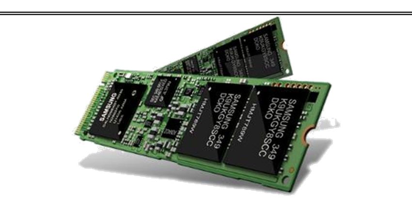
Recall: FLASH Memory

 Samsung 2015:
 512GB, NAND Flash
 • Like a normal transistor but:
 – Has a floating gate that can hold charge
 – To write: raise or lower wordline high enough to cause charges to tunnel
 – To read: turn on wordline as if normal transistor
 » presence of charge changes threshold and thus measured current
 • Two varieties:
 – NAND: denser, must be read and written in blocks
 – NOR: much less dense, fast to read and write
 • V-NAND: 3D stacking (Samsung claims 1TB possible in 1 chip)
4/5/2022 Joseph & Kubiatowicz CS162 © UCB Spring 2022 Lec 19.4

Recall: SSD Summary
 • Pros (vs. hard disk drives):
 – Low latency, high throughput (eliminate seek/rotational delay)
 – No moving parts:
 » Very light weight, low power, silent, very shock insensitive
 – Read at memory speeds (limited by controller and I/O bus)
 • Cons
 – Small storage (0.1-0.5x disk), expensive (3-20x disk)
 » Hybrid alternative: combine small SSD with large HDD

4/5/2022 Joseph & Kubiatowicz CS162 © UCB Spring 2022 Lec 19.5

Recall: SSD Summary
 • Pros (vs. hard disk drives):
 – Low latency, high throughput (eliminate seek/rotational delay)
 – No moving parts:
 » Very light weight, low power, silent, very shock insensitive
 – Read at memory speeds (limited by controller and I/O bus)No
 • Cons longer
 – Small storage (0.1-0.5x disk), expensive (3-20x disk) true!
 » Hybrid alternative: combine small SSD with large HDD
 – Asymmetric block write performance: read pg/erase/write pg
 » Controller garbage collection (GC) algorithms have major effect on performance
 – Limited drive lifetime
 » 1-10K writes/page for MLC NAND
 » Avg failure rate is 6 years, life expectancy is 9–11 years
 • These are changing rapidly!
4/5/2022 Joseph & Kubiatowicz CS162 © UCB Spring 2022 Lec 19.6

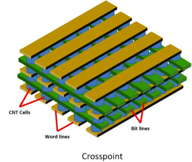
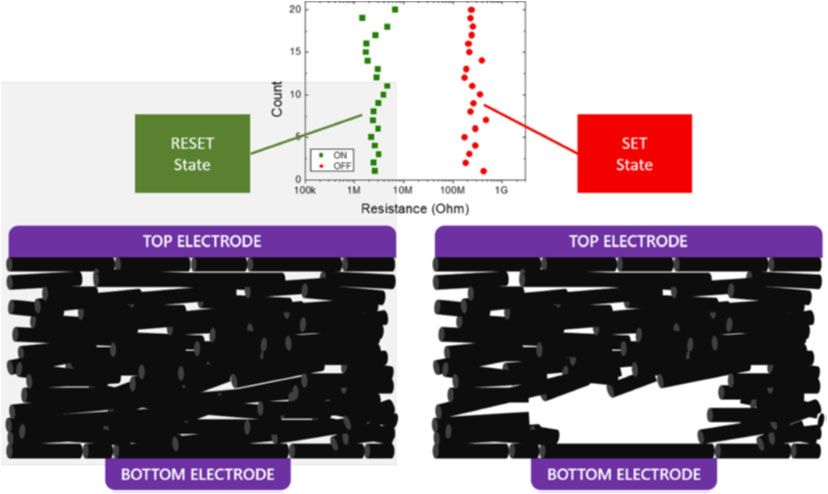
Nano-Tube Memory (NANTERO)

 • Yet another possibility: Nanotube memory
 – NanoTubes between two electrodes, slight conductivity difference between ones
 and zeros
 – No wearout!
 • Better than DRAM?
 – Speed of DRAM, no wearout, non-volatile!
 – Nantero promises 512Gb/dice for 8Tb/chip! (with 16 die stacking)
4/5/2022 Joseph & Kubiatowicz CS162 © UCB Spring 2022 Lec 19.7

Ways of Measuring Performance: Times (s) and Rates (op/s)
 • Latency – time to complete a task
 – Measured in units of time (s, ms, us, …, hours, years)
 • Response Time - time to initiate and operation and get its response
 – Able to issue one that depends on the result
 – Know that it is done (anti-dependence, resource usage)
 • Throughput or Bandwidth – rate at which tasks are performed
 – Measured in units of things per unit time (ops/s, GFLOP/s)
 • Start up or “Overhead” – time to initiate an operation
 • Most I/O operations are roughly linear in b bytes
 – Latency(b) = Overhead + b/TransferCapacity
 • Performance???
 – Operation time (4 mins to run a mile…)
 – Rate (mph, mpg, …)

4/5/2022 Joseph & Kubiatowicz CS162 © UCB Spring 2022 Lec 19.8

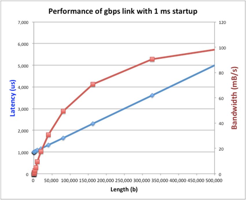
Example: Overhead in Fast Network
 • Consider a 1 Gb/s link ( 125 MB/s)
 with startup cost 1 ms
 • Latency: 
 • Effective Bandwidth:
 ⋅ 
 
 ⋅ ⋅ 
 1
 
 • Half-power Bandwidth: 
 • For this example, half-power bandwidth
 occurs at x 125 KB
 Length (x)

4/5/2022 Joseph & Kubiatowicz CS162 © UCB Spring 2022 Lec 19.9

Example: 10 ms Startup Cost (e.g., Disk)
 • Half-power bandwidth at x 1.25 MB Performance of gbps link with 10 ms startup
 18,000 50

 • Large startup cost can degrade 16,000 45

 effective bandwidth 14,000
 40

 35

 Bandwidth (mB/s)
 12,000

 Latency (us)
 30
 • Amortize it by performing I/O in larger 10,000

 blocks
 25
 8,000
 20

 6,000
 15

 4,000
 10

 2,000
 Half-power x = 1,250,000 bytes! 5

 0 0
 0 50,000 100,000 150,000 200,000 250,000 300,000 350,000 400,000 450,000 500,000
 Length
 Length(b)
 (x)

4/5/2022 Joseph & Kubiatowicz CS162 © UCB Spring 2022 Lec 19.10

What Determines Peak BW for I/O?
 • Bus Speed
 – PCI-X: 1064 MB/s = 133 MHz x 64 bit (per lane)
 – ULTRA WIDE SCSI: 40 MB/s
 – Serial Attached SCSI & Serial ATA & IEEE 1394 (firewire): 1.6 Gb/s full duplex
 (200 MB/s)
 – USB 3.0 – 5 Gb/s
 – Thunderbolt 3 – 40 Gb/s

 • Device Transfer Bandwidth
 – Rotational speed of disk
 – Write / Read rate of NAND flash
 – Signaling rate of network link

 • Whatever is the bottleneck in the path…

4/5/2022 Joseph & Kubiatowicz CS162 © UCB Spring 2022 Lec 19.11

Sequential Server Performance

 L L L L … L
 time

 • Single sequential “server” that can deliver a task in time operates at
 rate (on average, in steady state, …)
 op
 – 10 ms → 100 s
 op
 – 2 yr → 0.5 yr

 • Applies to a processor, a disk drive, a person, a TA, …

4/5/2022 Joseph & Kubiatowicz CS162 © UCB Spring 2022 Lec 19.12

Single Pipelined Server

 L L
 divided over distinct resources
 logical operation

 L L L L L L L
 …
 time
 • Single pipelined server of stages for tasks of length (i.e., time ⁄ per
 stage) delivers at rate ⁄.
 op
 – 10 ms, 4→ 400 s
 op
 – 2 yr, 2→ 1 yr

4/5/2022 Joseph & Kubiatowicz CS162 © UCB Spring 2022 Lec 19.13

Example Systems “Pipelines”

 I/O Processing

 syscall
 File Upper Lower
 User Process Driver Driver
 System
 Communication

 • Anything with queues between operational process behaves roughly
 “pipeline like”
 • Important difference is that “initiations” are decoupled from processing
 – May have to queue up a burst of operations
 – Not synchronous and deterministic like in 61C

4/5/2022 Joseph & Kubiatowicz CS162 © UCB Spring 2022 Lec 19.14

Multiple Servers

 L

 … k

 • servers handling tasks of length delivers at rate ⁄.
 op
 – 10 ms, 4→ 400 s
 op
 – 2 yr, 2→ 1 yr
 • In 61C you saw multiple processors (cores)
 – Systems present lots of multiple parallel servers
 – Often with lots of queues

4/5/2022 Joseph & Kubiatowicz CS162 © UCB Spring 2022 Lec 19.15

Example Systems “Parallelism”

 I/O Processing
 syscall File Upper Lower
 User Process
 User Process System Driver Driver
 User Process

 Communication

 Parallel Computation, Databases, …

4/5/2022 Joseph & Kubiatowicz CS162 © UCB Spring 2022 Lec 19.16

I/O Performance
 300 Response

 Controller
 Time (ms)
 User I/O
 device 200
 Thread
 Queue
 [OS Paths] 100
 Response Time = Queue + I/O device service time
 • Performance of I/O subsystem 0
 0% 100%
 – Metrics: Response Time, Throughput Throughput (% (Utilization)
 total BW)
 – Effective BW per op = transfer size / response time
 » EffBW(n) = n / (S + n/B) = B / (1 + SB/n )

 # of ops time per op

 Fixed overhead

4/5/2022 Joseph & Kubiatowicz CS162 © UCB Spring 2022 Lec 19.17

I/O Performance
 300 Response

 Controller
 Time (ms)
 User I/O
 device 200
 Thread
 Queue
 [OS Paths] 100
 Response Time = Queue + I/O device service time
 • Performance of I/O subsystem 0
 0% 100%
 – Metrics: Response Time, Throughput Throughput (% (Utilization)
 total BW)
 – Effective BW per op = transfer size / response time
 » EffBW(n) = n / (S + n/B) = B / (1 + SB/n )
 – Contributing factors to latency:
 » Software paths (can be loosely modeled by a queue)
 » Hardware controller
 » I/O device service time
 • Queuing behavior:
 – Can lead to big increases of latency as utilization increases
4/5/2022 – Solutions? Joseph & Kubiatowicz CS162 © UCB Spring 2022 Lec 19.18

A Simple Deterministic World

 arrivals Queue Server departures

 TQ TS
 TA TA TA

 Tq TS
 • Assume requests arrive at regular intervals, take a fixed
 time to process, with plenty of time between …
 • Service rate (μ = 1/TS) - operations per second
 • Arrival rate: (λ = 1/TA) - requests per second
 • Utilization: U = λ/μ , where λ < μ
 • Average rate is the complete story
4/5/2022 Joseph & Kubiatowicz CS162 © UCB Spring 2022 Lec 19.19

A Ideal Linear World
 Delivered Throughput

 Delivered Throughput
 Saturation
 1 1

 Empty Queue Unbounded
 0 1 0 1
 Offered Load (TS/TA) Offered Load (TS/TA)

 Queue delay
 Queue delay

 time time
 • What does the queue wait time look like?
 – Grows unbounded at a rate ~ (Ts/TA) till request rate subsides

4/5/2022 Joseph & Kubiatowicz CS162 © UCB Spring 2022 Lec 19.20

A Bursty World

 arrivals Queue Server departures

 TQ TS
 Arrivals

 Q depth

 Server

 • Requests arrive in a burst, must queue up till served
 • Same average arrival time, but almost all of the requests
 experience large queue delays
 • Even though average utilization is low
4/5/2022 Joseph & Kubiatowicz CS162 © UCB Spring 2022 Lec 19.21

So how do we model the burstiness of arrival?
 • Elegant mathematical framework if you start with
 exponential distribution
 – Probability density function of a continuous random variable
 with a mean of 1/λ
 – f(x) = λe-λx
 – “Memoryless” 1

 0.9

 Likelihood of an event 0.8

 occurring is independent of 0.7
 mean arrival interval (1/λ)
 0.6
 how long we’ve been waiting 0.5

 Lots of short arrival 0.4

 intervals (i.e., high 0.3

 0.2
 instantaneous rate) 0.1

 Few long gaps (i.e., low 0
 0 2 4 6 8 10
 instantaneous rate)
 x (λ)
4/5/2022 Joseph & Kubiatowicz CS162 © UCB Spring 2022 Lec 19.22

Background:
 General Use of Random Distributions
 Mean
 • Server spends variable time (T) with customers (m)
 
 – Mean (Average) m = p(T)T
 – Variance (stddev2) 2 = p(T)(T-m)2 = p(T)T2-m2
 – Squared coefficient of variance: C = 2/m2 Distribution
 Aggregate description of the distribution of service times

 • Important values of C: mean
 – No variance or deterministic  C=0
 – “Memoryless” or exponential  C=1
 » Past tells nothing about future Memoryless
 » Poisson process – purely or completely random process
 » Many complex systems (or aggregates)
 are well described as memoryless
 – Disk response times C  1.5 (majority seeks < average)

4/5/2022 Joseph & Kubiatowicz CS162 © UCB Spring 2022 Lec 19.23

Introduction to Queuing Theory

 Controller
 Disk
 Arrivals Queue Departures
 Queuing System

 • What about queuing time??
 – Let’s apply some queuing theory
 – Queuing Theory applies to long term, steady state behavior 
 Arrival rate = Departure rate

 • Arrivals characterized by some probabilistic distribution

 • Departures characterized by some probabilistic
 distribution
4/5/2022 Joseph & Kubiatowicz CS162 © UCB Spring 2022 Lec 19.24

Little’s Law

 arrivals N departures
 λ
 L
 • In any stable system
 – Average arrival rate = Average departure rate
 • The average number of jobs/tasks in the system (N) is equal to
 arrival time / throughput (λ) times the response time (L)
 – N (jobs) = λ (jobs/s) x L (s)
 • Regardless of structure, bursts of requests, variation in service
 – Instantaneous variations, but it washes out in the average
 – Overall, requests match departures
4/5/2022 Joseph & Kubiatowicz CS162 © UCB Spring 2022 Lec 19.25

Example

 L=5
 λ=1
 L=5

 N = 5 jobs

 Jobs

 0 1 2 3 4 5 6 7 8 9 10 11 12 13 14 15 16 time

 A: N = λ x L
 • E.g., N = λ x L = 5
4/5/2022 Joseph & Kubiatowicz CS162 © UCB Spring 2022 Lec 19.26

Little’s Theorem: Proof Sketch

 arrivals N departures
 λ
 L
 Job i L(i) = response time of job i
 N(t) = number of jobs in system
 at time t

 N(t)

 time
 L(1)
 T

4/5/2022 Joseph & Kubiatowicz CS162 © UCB Spring 2022 Lec 19.27

Little’s Theorem: Proof Sketch

 arrivals N departures
 λ
 L
 Job i L(i) = response time of job i
 N(t) = number of jobs in system
 at time t

 N(t)

 time
 T
 What is the system occupancy, i.e., average
 number of jobs in the system?
4/5/2022 Joseph & Kubiatowicz CS162 © UCB Spring 2022 Lec 19.28

Little’s Theorem: Proof Sketch

 arrivals N departures
 λ
 L
 Job i L(i) = response time of job i
 N(t) = number of jobs in system S(k)
 at time t
 S(i) = L(i) * 1 = L(i)

 N(t)

 S(2)
 S(1) time
 T

 S = S(1) + S(2) + … + S(k) = L(1) + L(2) + … + L(k)

4/5/2022 Joseph & Kubiatowicz CS162 © UCB Spring 2022 Lec 19.29

Little’s Theorem: Proof Sketch

 arrivals N departures
 λ
 L
 Job i L(i) = response time of job i
 N(t) = number of jobs in system
 at time t
 S(i) = L(i) * 1 = L(i)

 N(t)
 S= area

 time
 T

 Average occupancy (Navg) = S/T
4/5/2022 Joseph & Kubiatowicz CS162 © UCB Spring 2022 Lec 19.30

Little’s Theorem: Proof Sketch

 arrivals N departures
 λ
 L
 Job i L(i) = response time of job i
 N(t) = number of jobs in system S(k)
 at time t
 S(i) = L(i) * 1 = L(i)

 N(t)

 S(2)
 S(1) time
 T

 Navg = S/T = (L(1) + … + L(k))/T

4/5/2022 Joseph & Kubiatowicz CS162 © UCB Spring 2022 Lec 19.31

Little’s Theorem: Proof Sketch

 arrivals N departures
 λ
 L
 Job i L(i) = response time of job i
 N(t) = number of jobs in system S(k)
 at time t
 S(i) = L(i) * 1 = L(i)

 N(t)

 S(2)
 S(1) time
 T
 Navg = (L(1) + … + L(k))/T = (Ntotal/T)*(L(1) + … + L(k))/Ntotal

4/5/2022 Joseph & Kubiatowicz CS162 © UCB Spring 2022 Lec 19.32

Little’s Theorem: Proof Sketch

 arrivals N departures
 λ
 L
 Job i L(i) = response time of job i
 N(t) = number of jobs in system S(k)
 at time t
 S(i) = L(i) * 1 = L(i)

 N(t)

 S(2)
 S(1) time
 T

 Navg = (Ntotal/T)*(L(1) + … + L(k))/Ntotal = λavg × Lavg

4/5/2022 Joseph & Kubiatowicz CS162 © UCB Spring 2022 Lec 19.33

Little’s Theorem: Proof Sketch

 arrivals N departures
 λ
 L
 Job i L(i) = response time of job i
 N(t) = number of jobs in system S(k)
 at time t
 S(i) = L(i) * 1 = L(i)

 N(t)

 S(2)
 S(1) time
 T

 Navg = λavg × Lavg

4/5/2022 Joseph & Kubiatowicz CS162 © UCB Spring 2022 Lec 19.34

Little’s Law Applied to a Queue

 • When Little’s Law applied to a queue, we get:

 Average Arrival Rate

 Average length of Average time “waiting”
 the queue in queue

4/5/2022 Joseph & Kubiatowicz CS162 © UCB Spring 2022 Lec 19.35

A Little Queuing Theory: Computing TQ
 • Assumptions: Why does response/queueing
 – System in equilibrium; No limit to the queue
 delay grow unboundedly even
 – Time between successive arrivals is random and memoryless
 though the utilization is < 1 ?
 Queue Server 300 Response
 Arrival Rate Service Rate Time (ms)
  μ=1/Tser
 200
 • Parameters that describe our system:
 – : mean number of arriving customers/second 100
 – Tser: mean time to service a customer (“m1”)
 – C: squared coefficient of variance = 2/m12 0 100%
 – μ: service rate = 1/Tser 0%
 – u: server utilization (0u1): u = /μ =   Tser Throughput (Utilization)
 (% total BW)
 • Results:
 – Memoryless service distribution (C = 1): (an “M/M/1 queue”):
 » Tq = Tser x u/(1 – u)
 – General service distribution, 1 server (an “M/G/1 queue”):
 » Tq = Tser x ½(1+C) x u/(1 – u)
4/5/2022 Joseph & Kubiatowicz CS162 © UCB Spring 2022 Lec 19.36

System Performance In presence of a Queue
 Latency ( ) • ~ ,u ⁄
 Service Rate ( )

 • Why does latency
 blow up as we
 - “delivered

 approach 100%
 Time

 utilization?
 load”

 • Queue builds up on
 each burst
 Operation Time • But very rarely (or
 Request Rate ( ) - “offered load” never) gets a
 chance to drain

 “Half-Power Point” : load at which system delivers half of peak performance
 - Design and provision systems to operate roughly in this regime
 - Latency low and predictable, utilization good: ~50%

4/5/2022 Joseph & Kubiatowicz CS162 © UCB Spring 2022 Lec 19.37

Why unbounded response time?
 • Assume deterministic arrival process and service time
 – Possible to sustain utilization = 1 with bounded response time!

 time

 arrival service
 time time

4/5/2022 Joseph & Kubiatowicz CS162 © UCB Spring 2022 Lec 19.38

Why unbounded response time?
 300 Response
 • Assume stochastic arrival process Time (ms)
 (and service time)
 200
 – No longer possible to achieve
 utilization = 1 100

 This wasted time can
 0 100%
 never be reclaimed! 0%
 Throughput (Utilization)
 So cannot achieve u = 1! (% total BW)

 time

4/5/2022 Joseph & Kubiatowicz CS162 © UCB Spring 2022 Lec 19.39

A Little Queuing Theory: An Example
 • Example Usage Statistics:
 – User requests 10 x 8KB disk I/Os per second
 – Requests & service exponentially distributed (C=1.0)
 – Avg. service = 20 ms (From controller+seek+rot+trans)
 • Questions:
 – How utilized is the disk?
 » Ans: server utilization, u = Tser
 – What is the average time spent in the queue?
 » Ans: Tq
 – What is the number of requests in the queue?
 » Ans: Lq
 – What is the avg response time for disk request?
 » Ans: Tsys = Tq + Tser
 • Computation:
  (avg # arriving customers/s) = 10/s
 Tser (avg time to service customer) = 20 ms (0.02s)
 u (server utilization) =  x Tser= 10/s x .02s = 0.2
 Tq (avg time/customer in queue) = Tser x u/(1 – u)
 = 20 x 0.2/(1-0.2) = 20 x 0.25 = 5 ms (0 .005s)
 Lq (avg length of queue) =  x Tq=10/s x .005s = 0.05
 Tsys (avg time/customer in system) =Tq + Tser= 25 ms
4/5/2022 Joseph & Kubiatowicz CS162 © UCB Spring 2022 Lec 19.40

Queuing Theory Resources
 • Resources page contains Queueing Theory Resources (under
 Readings):
 – Scanned pages from Patterson and Hennessy book that gives further
 discussion and simple proof for general equation:
 https://cs162.eecs.berkeley.edu/static/readings/patterson_queue.pdf
 – A complete website full of resources:
 http://web2.uwindsor.ca/math/hlynka/qonline.html

 • Some previous midterms with queueing theory questions

 • Assume that Queueing Theory is fair game for Midterm III!

4/5/2022 Joseph & Kubiatowicz CS162 © UCB Spring 2022 Lec 19.41

Optimize I/O Performance
 Response

 Controller
 300
 Time (ms)
 User I/O
 Thread device
 200
 Queue
 [OS Paths]
 100
 Response Time =
 Queue + I/O device service time
 0 100%
 • How to improve performance? 0%
 Throughput (Utilization)
 – Make everything faster  (% total BW)
 – More Decoupled (Parallelism) systems
 » multiple independent buses or controllers
 – Optimize the bottleneck to increase service rate
 » Use the queue to optimize the service
 – Do other useful work while waiting
 • Queues absorb bursts and smooth the flow
 • Admissions control (finite queues)
 – Limits delays, but may introduce unfairness and livelock
4/5/2022 Joseph & Kubiatowicz CS162 © UCB Spring 2022 Lec 19.42

When is Disk Performance Highest?
 • When there are big sequential reads, or
 • When there is so much work to do that they can be piggy
 backed (reordering queues—one moment)

 • OK to be inefficient when things are mostly idle
 • Bursts are both a threat and an opportunity
 • 
 – Waste space for speed?

 • Other techniques:
 – Reduce overhead through user level drivers
 – Reduce the impact of I/O delays by doing other useful work
 in the meantime

4/5/2022 Joseph & Kubiatowicz CS162 © UCB Spring 2022 Lec 19.43

Disk Scheduling (1/3)
 • Disk can do only one request at a time; What order do you
 choose to do queued requests?
 User

 2,2
 5,2
 7,2
 3,10
 2,1
 2,3
 Head
 Requests

 • FIFO Order
 – Fair among requesters, but order of arrival may be
 to random spots on the disk  Very long seeks
 • SSTF: Shortest seek time first

 Disk Head
 – Pick the request that’s closest on the disk
 3
 – Although called SSTF, today must include
 rotational delay in calculation, since 2
 1
 rotation can be as long as seek
 – Con: SSTF good at reducing seeks, but 4
 may lead to starvation

4/5/2022 Joseph & Kubiatowicz CS162 © UCB Spring 2022 Lec 19.44

Disk Scheduling (2/3)
 • Disk can do only one request at a time; What order do you
 choose to do queued requests?
 User

 2,2
 5,2
 7,2
 3,10
 2,1
 2,3
 Head
 Requests

 • SCAN: Implements an Elevator Algorithm: take the closest
 request in the direction of travel
 – No starvation, but retains flavor of SSTF

4/5/2022 Joseph & Kubiatowicz CS162 © UCB Spring 2022 Lec 19.45

Disk Scheduling (3/3)
 • Disk can do only one request at a time; What order do you
 choose to do queued requests?
 User

 2,2
 5,2
 7,2
 3,10
 2,1
 2,3
 Head
 Requests

 • C-SCAN: Circular-Scan: only goes in one direction
 – Skips any requests on the way back
 – Fairer than SCAN, not biased towards pages in middle

4/5/2022 Joseph & Kubiatowicz CS162 © UCB Spring 2022 Lec 19.46

Recall: How do we Hide I/O Latency?
 • Blocking Interface: “Wait”
 – When request data (e.g., read() system call), put process to sleep until
 data is ready
 – When write data (e.g., write() system call), put process to sleep until
 device is ready for data
 • Non-blocking Interface: “Don’t Wait”
 – Returns quickly from read or write request with count of bytes
 successfully transferred to kernel
 – Read may return nothing, write may write nothing
 • Asynchronous Interface: “Tell Me Later”
 – When requesting data, take pointer to user’s buffer, return
 immediately; later kernel fills buffer and notifies user
 – When sending data, take pointer to user’s buffer, return immediately;
 later kernel takes data and notifies user
4/5/2022 Joseph & Kubiatowicz CS162 © UCB Spring 2022 Lec 19.47

Recall: I/O and Storage Layers

 Application / Service

 High Level I/O Streams

 Low Level I/O File Descriptors What we covered in Lecture 4
 Syscall open(), read(), write(), close(), …
 Open File Descriptions
 File System Files/Directories/Indexes What we will cover next…
 I/O Driver Commands and Data Transfers

 Disks, Flash, Controllers, DMA
 What we just covered…

4/5/2022 Joseph & Kubiatowicz CS162 © UCB Spring 2022 Lec 19.48

From Storage to File Systems

 I/O API and Memory Address
 Variable-Size Buffer
 syscalls

 Logical Index,
 File System Block Typically 4 KB

 Flash Trans. Layer
 Hardware
 Sector(s)
 Sector(s)
 Devices Sector(s) Phys Index.,
 Phys. Block
 4KB
 Physical Index,
 512B or 4KB Erasure Page

 HDD SSD

4/5/2022 Joseph & Kubiatowicz CS162 © UCB Spring 2022 Lec 19.49

Building a File System
 • File System: Layer of OS that transforms block interface of disks (or other
 block devices) into Files, Directories, etc.
 • Classic OS situation: Take limited hardware interface (array of blocks) and
 provide a more convenient/useful interface with:
 – Naming: Find file by name, not block numbers
 – Organize file names with directories
 – Organization: Map files to blocks
 – Protection: Enforce access restrictions
 – Reliability: Keep files intact despite crashes, hardware failures, etc.

4/5/2022 Joseph & Kubiatowicz CS162 © UCB Spring 2022 Lec 19.50

Recall: User vs. System View of a File
 • User’s view:
 – Durable Data Structures
 • System’s view (system call interface):
 – Collection of Bytes (UNIX)
 – Doesn’t matter to system what kind of data structures you want to store on disk!
 • System’s view (inside OS):
 – Collection of blocks (a block is a logical transfer unit, while a sector is the physical
 transfer unit)
 – Block size  sector size; in UNIX, block size is 4KB

4/5/2022 Joseph & Kubiatowicz CS162 © UCB Spring 2022 Lec 19.51

Translation from User to System View

 File File
 (Bytes) System

 • What happens if user says: “give me bytes 2 – 12?”
 – Fetch block corresponding to those bytes
 – Return just the correct portion of the block
 • What about writing bytes 2 – 12?
 – Fetch block, modify relevant portion, write out block
 • Everything inside file system is in terms of whole-size blocks
 – Actual disk I/O happens in blocks
 – read/write smaller than block size needs to translate and buffer

4/5/2022 Joseph & Kubiatowicz CS162 © UCB Spring 2022 Lec 19.52

Disk Management
 • Basic entities on a disk:
 – File: user-visible group of blocks arranged sequentially in logical space
 – Directory: user-visible index mapping names to files

 • The disk is accessed as linear array of sectors
 • How to identify a sector?
 – Physical position
 » Sectors is a vector [cylinder, surface, sector]
 » Not used anymore
 » OS/BIOS must deal with bad sectors
 – Logical Block Addressing (LBA)
 » Every sector has integer address
 » Controller translates from address  physical position
 » Shields OS from structure of disk

4/5/2022 Joseph & Kubiatowicz CS162 © UCB Spring 2022 Lec 19.53

What Does the File System Need?
 • Track free disk blocks
 –Need to know where to put newly written data
 • Track which blocks contain data for which files
 –Need to know where to read a file from
 • Track files in a directory
 –Find list of file's blocks given its name
 • Where do we maintain all of this?
 –Somewhere on disk

4/5/2022 Joseph & Kubiatowicz CS162 © UCB Spring 2022 Lec 19.54

Conclusion
 • Disk Performance:
 – Queuing time + Controller + Seek + Rotational + Transfer
 – Rotational latency: on average ½ rotation
 – Transfer time: spec of disk depends on rotation speed and bit storage density
 • Devices have complex interaction and performance characteristics
 – Response time (Latency) = Queue + Overhead + Transfer
 » Effective BW = BW * T/(S+T)
 – HDD: Queuing time + controller + seek + rotation + transfer
 – SDD: Queuing time + controller + transfer (erasure & wear)
 • Systems (e.g., file system) designed to optimize performance and reliability
 – Relative to performance characteristics of underlying device
 • Bursts & High Utilization introduce queuing delays
 • Queuing Latency:
 – M/M/1 and M/G/1 queues: simplest to analyze
 – As utilization approaches 100%, latency  
 Tq = Tser x ½(1+C) x u/(1 – u))
4/5/2022 Joseph & Kubiatowicz CS162 © UCB Spring 2022 Lec 19.55