Computational identification of 4 carboxyglutamate sites to supplement physiological studies using deep learning
←
→
Page content transcription
If your browser does not render page correctly, please read the page content below
www.nature.com/scientificreports
OPEN Computational identification
of 4‑carboxyglutamate sites
to supplement physiological
studies using deep learning
Sheraz Naseer1, Rao Faizan Ali1,2*, Suliman Mohamed Fati3 & Amgad Muneer2
In biological systems, Glutamic acid is a crucial amino acid which is used in protein biosynthesis.
Carboxylation of glutamic acid is a significant post-translational modification which plays important
role in blood coagulation by activating prothrombin to thrombin. Contrariwise, 4-carboxy-glutamate
is also found to be involved in diseases including plaque atherosclerosis, osteoporosis, mineralized
heart valves, bone resorption and serves as biomarker for onset of these diseases. Owing to the
pathophysiological significance of 4-carboxyglutamate, its identification is important to better
understand pathophysiological systems. The wet lab identification of prospective 4-carboxyglutamate
sites is costly, laborious and time consuming due to inherent difficulties of in-vivo, ex-vivo and
in vitro experiments. To supplement these experiments, we proposed, implemented, and evaluated
a different approach to develop 4-carboxyglutamate site predictors using pseudo amino acid
compositions (PseAAC) and deep neural networks (DNNs). Our approach does not require any feature
extraction and employs deep neural networks to learn feature representation of peptide sequences
and performing classification thereof. Proposed approach is validated using standard performance
evaluation metrics. Among different deep neural networks, convolutional neural network-based
predictor achieved best scores on independent dataset with accuracy of 94.7%, AuC score of 0.91
and F1-score of 0.874 which shows the promise of proposed approach. The iCarboxE-Deep server is
deployed at https://share.streamlit.io/sheraz-n/carboxyglutamate/app.py.
Cells, the fundamental units of life, experience different physiological phenomena during their lifecycle which
give rise to the dynamic changes in their structure and functions. One such phenomenon is post-translational
modification of proteins, the complex molecules, which are found in nearly all aspects of cell’s l ife1. An important
post-translational-modification (PTM) is 4-Carboxyglutamate (CarboxE), synthesized by replacing a proton from
4-carbon of glutamate with carboxyl group2. 4-Carboxyglutamate plays pivotal role in the blood clotting cascade
specifically occurring in Coagulation factors II, VII, IX, and X, protein C, protein S, and some bone p roteins3.
Aforementioned coagulation factors are dependent on Vitamin-K, a cofactor for carboxylase, which serves as
a catalyst for CO 2 addition on glutamate peptide for c arboxylation4. Oxygenation of vitamin K hydroquinone
is catalyzed by Vitamin K-dependent carboxylase, a bi-functional enzyme, enabling the creation of vitamin K
epoxide which forms c arboxyglutamate5. Furthermore, a key part is played by CarboxE in calcium dependent
interaction between prothrombin and negatively charged phospholipid surface, which is pivotal for activation
of prothrombin to thrombin6. CarboxE is found to have significantly lower mean disorder scores than their
unmodified counterparts and the modified residues showed lower mean spatial fluctuations than unmodified
residues7. The CarboxE containing proteins of hepatic origins are characterized by their role in blood coagula-
tion while non-hepatic proteins containing same PTM, e.g. osteocalcin and atherocalcin, are known for their
calcium binding properties8. Additionally, the small amounts of osteocalcin and other CarboxE containing
proteins are found to occur in calcified atherosclerotic lesions and mineralized heart valves9. Due to its calcium
binding properties, CarboxE is also considered a biomarker for diseases including osteoporosis, papilloma, bone
resorption and plaque a therosclerosis3,5.
1
Department of Computer Science, University of Management and Technology, Lahore 54770,
Pakistan. 2Computer and Information Sciences Department, Universiti Teknologi PETRONAS, 32610 Seri
Iskandar, Malaysia. 3College of Computer and Information Sciences, Prince Sultan University, Riyadh 11586, Saudi
Arabia. *email: faizan.ali@umt.edu.pk
Scientific Reports | (2022) 12:128 | https://doi.org/10.1038/s41598-021-03895-4 1
Vol.:(0123456789)
www.nature.com/scientificreports/
Figure 1. Chou’s five step methodology.
Owing to the importance of CarboxE in physiological phenomena, research has been done on identification of
carboxylation sites using mass spectrometric analysis10. But due to huge cost and effort requirements for in-vivo,
ex-vivo and in-vitro identification of CarboxE, scarce effort is put in wet lab identification of the same. Mean-
while, in-silico methods, based on machine learning and data science, showed a promising avenue to characterize
CarboxE sites to supplement wet lab methods. In fact, researchers have applied in-silico methods to support
the wet lab experiments in proteomics and genomics using various machine learning and artificial intelligence
techniques11–17. Prior literature proposed various computational methods to identify glutamate carboxylation5,18.
While these contributions show promise, the proposed computational models were based on human-engineered
features. According to Lecun et al.19, human-engineered features suffer from certain limitations as they are diffi-
cult to calculate because of absence of a feedback mechanism between prediction algorithm and feature extraction
mechanism. The absence of feedback system hinders the development of an effective predictor because there is
no way to evaluate the quality of features beforehand. Additionally, generation of human-engineered features
require domain knowledge and human intervention which is costly to a chieve19.
Modern deep learning offers a very powerful framework for solving learning problems. When a Deep Neu-
ral Network (DNN) is sufficiently trained on input/output pairs of peptide sequences and labels, it is able to
reduce the input sequence, by performing hierarchical input transformations through trained hidden layers
of neurons, into the correct label for given input peptide sequence. DNNs do not require prior feature extrac-
tion, because the deep model can automatically learn the low-dimensional, task specific and optimal feature
representation from hierarchical non-linear transformations of original pseudo Amino ACID Composition
(PseAAC) sequences. These abstract, task specific deep neural representations are used by the output layer, which
is usually composed of any classifier like sigmoid or softmax, to make p redictions20–22. In effect, deep learning
is gaining popularity for solving the proteomics and genomics problems due to non-requirement of prior costly
feature extraction23–25. Deep learning provides a highly powerful framework for handling learning challenges
in the modern-day. Although, the majority of the works for PTM prediction are comprised of conventional
machine-learning-based feature extraction methodology, deep learning is gaining popularity to solve proteom-
ics and genomics problems due to the non-requirement of prior costly feature e xtraction14,26,27. Deep learning
based models are far more efficient and provide results comparable conventional Machine-learning predictors
as demonstrated in22,26,27. Another significant advantage of deep learning is lack of need for Feature-engineering
or extraction because DNNs can work with raw inputs. Our methodology uses DNN based approach to iden-
tify potential CarboxE sites and will make sure that devised improvements are met in the best possible way. In
contrast to previously proposed conventional ML based predictors, which rely on quality of features, the current
analysis aims to devise an in-silico approach for CarboxE site prediction by fusing DNNs with Chou’s five-step
rule28 as presented in Fig. 1 and used extensively by previous s tudies5,11–17.
Results
In this research, DNNs-based model performance is evaluated using well-known evaluation metrics. The critical
evaluation metrics employed in this study include the receiver operating characteristics learning curve (ROC),
precision-recall, Area under Curve, accuracy, and matthew’s correlation coefficient to name a few. A brief descrip-
tion of above-mentioned metrics is discussed in following section . The five proposed DNNs models are evaluated
and tested on the testing data set, which is not exposed to models throughout the training process, to guarantee
fair estimation of generalization capability. The following subsections offers evaluation results of DNN based
predictors for identifying CarboxE sites developed in this study. Figure 2 illustrates the precision-recall curve of
candidate DNN based predictors. As depicted in Fig. 2, the CNN model’s curve is closest in the precision-recall
space to the perfect prediction point (1, 1) compared to that of the other classifiers, demonstrating the better
performance of the CNN classifier model. In comparison to the aforementioned CNN based model, all the other
DNN-based classifiers performed below par, as shown by their respective curves, which are comparatively far
from the perfect classification point. To represent the findings of precision-recall curve in a single scalar value,
mean average precision (mAP) is used which is defined as the region under the precision-recall curve. The higher
the mAP score of the classifier, the greater the classifier’s prediction efficiency and vice versa. For all candidate
CarboxE site prediction models, the mean average precision (mAP) scores for DNN models are presented in the
legend portion of Fig. 2. As illustrated in aforementioned figure, the CNN-based model achieved the best score
of 0.937 and LSTM achieved the best second score with a value of 0.876. Meanwhile, FCN fell short and obtained
the lowest score of 0.723. Overall, the DNN models utilized in this study achieved a score higher than 70%.
Scientific Reports | (2022) 12:128 | https://doi.org/10.1038/s41598-021-03895-4 2
Vol:.(1234567890)
www.nature.com/scientificreports/

                                 Figure 2.  Precision-recall curve and mAP scores DNN-based CarboxE site prediction models.

                                 Figure 3.  ROC curve and AUC scores for DNN based CarboxE site identification models.

Scientific Reports |   (2022) 12:128 |              https://doi.org/10.1038/s41598-021-03895-4                                     3

                                                                                                                              Vol.:(0123456789)
www.nature.com/scientificreports/
Figure 4. Accuracy, F1-measure, and MCC scores of DNN-based CarboxE site prediction models.
Receiver operating characteristics and area under ROC curve. The ROC curves for the proposed
five DNN based CarboxE predictors, built in this study, are introduced in Fig. 3. It can be seen from the afore-
mentioned figure that the curve of the CNN-based predictor is nearest to the perfect classification point as
compared to that of remaining DNN based models, demonstrating the better performance of the CNN-based
model. The AUC values for the models built in this analysis are presented in the Legend portion of Fig. 3. It is
shown clearly from the aforementioned figure that the CNN based model outperforms the rest of the methods
in predicting CarboxE sites, with an AUC value of 0.971. The FCN model obtained the second-best prediction
with an AUC value of 0.922. The results of the ROC curve corroborate the earlier evaluation results indicated by
the precision-recall curve.
Accuracy, F1‑measure, and Matthew Correlation Coefficient. The accuracy score of CarboxE iden-
tification models, calculated using independent testset, are illustrated in Fig. 4. From the aforementioned figure,
it is evident that the accuracy score of CNN-based predictor dominated remaining all predictors developed in
this study with score of 0.947 followed by 0.908 score of GRU and S-RNN based models. Although the accuracy
results are trust-worthy for balanced datasets, it can be misleading when an imblanace exists in data points of
different classes in a dataset. To mitigate the possibility of its spurious findings, accuracy is often used in con-
junction with F1 score or matthew’s correlation coefficient. The F1-measurements of CarboxE identification
models are also depicted in Fig. 4 and the results validate the domineering performance of CNN-based model
which showed F1-score of 0.874 while S-RNN model remained the runner-up with F1-measurement of 0.828.
GRU and LSTM based models showed comparable performance and achieved an F1 score of 0.820 and 0.814,
respectively. FCN score wasn’t that far from the aforementioned DNNs but achieved last place nonetheless with
F1-score of 0.798. The outcomes of MCC for all DNN dependent models, proposed in this study, are shown in
Fig. 4. Based on MCC, the CNN-based model achieved best performance rate of 0.825, followed by the S-RNN-
based and GRU-based models achieving a performance rate of 0.747 and 0.740. Lastly, the FCN-based model
obtained the least performance score of 0.708 in terms of MCC evaluation matric. From the performance of
CNN based model in all three point metrics discussed in this section, it is evident from the evaluation scores
that CNN based model showed promising performance and surpassed other DNN based model developed dur-
ing this study.
Comparison with literature. This subsection discusses the comparison of proposed approach with simi-
lar contributions from literature as well the prospective reasons for better performance of DNNs for identifica-
tion of CarboxE sites. Identification of CarboxE using machine learning and other in-silico methods is rela-
tively ignored area of research by bioinformatics community and we were able to find only one contribution
for in-silico prediction of 4-carboxyglutamate by Shah et al.5. Shah et al. used statistical moments and residue
position related techniques to extract features form the peptide sequences and used these features to train their
4-carboxyglutamate predictor. The comparison of our best model i.e. CNN based model with system proposed
by5 is presented in Table 1 on the basis of standard performance evaluation metrics. It can be seen from Table 1
that the model proposed by Ref.5 is performing almost as good as the proposed predictor. The reader may feel
that if the predictor developed by Ref.5 is performing comparable to proposed approach then there is little merit
in using the DNNs for the problem at hand. This is not the case owing to the following benefits provided by
proposed approach:
Scientific Reports | (2022) 12:128 | https://doi.org/10.1038/s41598-021-03895-4 4
Vol:.(1234567890)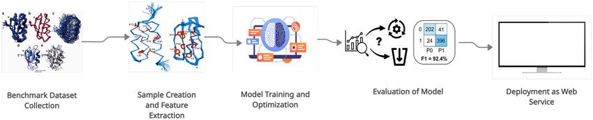
www.nature.com/scientificreports/
Performance evaluation metric Proposed CNN based model Reported results by5
Accuracy 0.947 0.94
AUC 0.971 0.96
F1-score 0.874 Not reported
MCC 0.825 0.85
Sensitivity 0.923 0.92
Specificity 0.918 0.93
mAP 0.945 Not reported
Table 1. Comparison with available literature.
• Human engineered feature extraction is generally more expensive and requires human experts to develop and
validate the features. The system proposed by Ref.5 uses statistical moments and position incidence which
are costly to extract, needs expert domain knowledge and human intervention to achieve better results5.
• Deep features, as used in current study, are more advantageous than human engineered features because they
do not require any human intervention and are easily extractable, once the deep model is trained. The deep
features can be extracted efficiently by a forward pass through the trained DNN.
• Deep features are usually simpler and more effective than their human engineered counterparts because, in
DNNs, the feature extraction and classification work in unison to extract the features which help to achieve
better features for classification. This is evident form fact that the proposed CNN based approach, in this
study, uses 8 deep features (extracted from last fully connected layer of CNN) to achieve comparable clas-
sification results to the system proposed by Shah et al.5 which uses more than 100 human engineered features
to train classifiers.
Aforementioned facts illustrate the merits of DNN based prediction of CarboxE sites and compel us to consider
DNN based model an effective and efficient alternative for rather expensive approaches utilizing human engi-
neered features22.
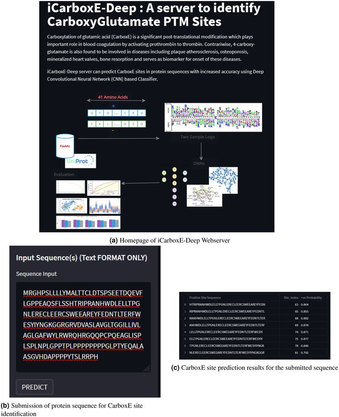
Model deployment as webserver. Final step of Chou’s 5-step rule as shown in Fig. 1 is the deployment of
developed model as a web service to enable easy access for research community. To this end, we developed a web
application based on our best performing CNN based model for identification of CarboxE sites. The webserver
is temporarily deployed at https://share.streamlit.io/sheraz-n/carboxyglutamate/app.py. The web application can
accept a peptide sample in the form of string and return the identified glutamic acid sites likely to be carboxy-
lated. Homepage of iCarboxE-Deep webserver is shown in Fig. 5a while Fig. 5b highlights the peptide sequence
submission process for computing CarboxE sites. Figure 5c illustrates result page showing the identified glu-
tamic acid sites likely to be carboxylated and the corresponding ξ = 41 length PseAAC sequence of residues.
Discussion
For understanding deep feature representations of peptide sequences, learned by DNNs to predict CarboxE
sites, visualizing these feature spaces can provide an intuitive understanding of why these feature representations
work. To create these visualizations, we calculated the output of penultimate layer of each trained model using
testset peptide sequences and extrapolated the 2-D projections of the same using t-stochastic neighborhood
embeddings (t-SNE) algorithm, developed by Maaten and H inton29. T-SNE makes use of non-linear statistical
approach to extrapolate 2-D projections of deep features calculated from non-linearly transformed input peptide
sequences. T-SNE uses many hyperparameters including perplexity, initialization and iterations to develop the
projections in lower dimensions. Since our testset contained only 308 samples with maximum 41 dimensions for
raw sequences and 8 dimensions for deep representations, the recommended range for perplexity is 0–50. We
used default perplexity value of 30 for scikit-learn t-SNE implementation30, used PCA initialization for efficient
dimensionality reduction and fixed the iterations to 1000 for calculating the 2-D projections of deep features. The
developed 2-D projections of deep models were plotted on the basis of class labels using matplotlib and seaborn
package of python. Fig. 6a–d show the aforementioned visualizations of PseAAC sequences and feature space
representations learned by the deep models developed in this study. Visualization of Raw PseAAC sequences, as
visible in Fig. 6a, shows the distribution of positive and negative CarboxE samples without any feature extraction.
As illustrated in the figure, the samples from both classes are cluttered over the space and no clear boundary
exists between samples of two classes. This chaotic distribution suggests that any classifier aiming to separate
samples of both classes while using this representation will have a hard time doing so. Figure 6b–d depict the
effect of non-linear transformations of three DNNs, used in this study, to separate both classes in respective
feature space for achieving better predictions. The visualization plots included in manuscript corresponds to one
low performance model i.e FCN and two optimal models including LSTM and CNN based models. The FCN
feature space visualization is shown in Fig. 6b. It can be verified from aforementioned figure that this model was
not sufficiently successful in separating the positive and negative samples before passing their representation to
output layer which resulted in poor performance of respective predictor. The best class separation is achieved
by the input representation learned by CNN model as shown in Fig. 11. The data distribution of positive and
Scientific Reports | (2022) 12:128 | https://doi.org/10.1038/s41598-021-03895-4 5
Vol.:(0123456789)
www.nature.com/scientificreports/

                                           Figure 5.  iCarboxE-Deep Webserver functionalities for identification of 4-carboxy-glutamate.

                                           negative samples in CNN representation is illustrated in violin plot shown by Fig. 7. It is evident from Figs. 6d
                                           and 7 that this representation is not chaotic and cluttered and both classes are sufficiently separated to make the
                                           job of classifier comparatively easier. This means any classifier consuming this representation to predict CarboxE
                                           sites will be able to distinguish between both classes with less effort and achieve better predictions. This is also
                                           corroborated by the better results shown by CNN based predictor as discussed in “Results”.
                                               The major benefit of DNN based approach proposed in this study is the automatic feature representation
                                           learning using stochastic gradient decent. Proposed approach removes the requirement to use costly feature
                                           engineering process. Moreover, the proposed DNN based predictor of this study are only the first step towards
                                           employing deep learning for 4-Carboxyglutamate site identification and research community can extend
                                           this study to come up with more effective in-silico systems using deep learning for 4-Carboxyglutamate site
                                           identification.

          Scientific Reports |   (2022) 12:128 |                https://doi.org/10.1038/s41598-021-03895-4                                                   6

Vol:.(1234567890)
www.nature.com/scientificreports/
Figure 6. Feature space visualizations of deep representations for positive and negative CarboxE sample.
Materials and methods
The suggested approach for this study, as shown in Fig. 8, is derived from the five-step rule of Chou28, popular in
proteomics research31,32. However, instead of depending on human-engineered features, the proposed approach
employs DNNs for combining feature extraction and model training to extract features and train models and
use the intrinsic capabilities of DNN’s feature extraction and classification. If the DNN model is satisfactorily
trained, the hidden layers of DNN perform processing on PseAAC peptide sequences to calculate effective deep
representations, which are then utilized by the DNN’s output layer to perform prediction. The loss score is used
as a feedback signal by the optimizer to enhance both the feature extraction and classification capability of the
model. In this study, several DNN-based models have been trained and tested to arrive at an optimal model for
predicting CarboxE sites. This section’s key purpose is to elaborate the first three phases presented in Fig. 8, while
rest have been explained in previous sections.
Benchmark dataset collection. We utilized the advanced search and annotation features in UniProt33 to
produce a dataset for conducting the proposed study. The benchmark dataset’s consistency has been ensured by
choosing protein sequences that are experimentally investigated and evaluated. Selected proteins were subjected
through CD-Hit34 to remove the homology with a threshold of 0.8. Resulting proteins were used to extract posi-
tive and negative sequences for CarboxE sites. The PseAAC representation of a peptide sequence containing a
positive CarboxE site may be described as follows:
fǫ (P) = k−ǫ k−(ǫ−1) . . . k−2 k−1 Ek+1 k+2 . . . k+(ǫ−1) , k+ǫ
where ‘E’ denotes PTM site for CarboxE and ‘k’ represents the neighbor amino acid residues of positive site.
Respectively, the Greek letter ǫ describes the indexes of PseAAC sequence residues, where the left-hand residues
of CarboxE site are located at negative ǫ indexes, and the right-hand residues are located at their respective
positive ǫ indexes. To develop a benchmark dataset, the length ξ for both negative and positive samples were
extracted from experimentally verified proteins. Based on empirical observations and literature support5,26,27,
the length ξ is set at 41 for negative and positive samples equally. Each positive sample is created via setting the
index of the CarboxE site at 21 and collecting 20 left and 20 right neighbor residues of the positive side, which
resulted in the standard ξ length sequence. For sequences with ξ < 41, a dummy residue symbol ‘X’ is placed on
both sequence sides to obtain the standard length. Similar approach was utilized to develop the negative samples
from aforementioned experimentally verified proteins, where the only difference is the presence of non-CarboxE
glutamate at sequence index ǫ = 21 rather than CarboxE site. Using the above process, we were able to get 308
positive and 617 negative samples. The final benchmark dataset comprised of 308 positive and randomly chosen
617 negative samples making a total of 925 samples. The final dataset can be represented as follows:
Scientific Reports | (2022) 12:128 | https://doi.org/10.1038/s41598-021-03895-4 7
Vol.:(0123456789)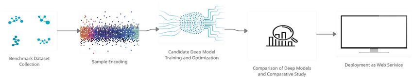
www.nature.com/scientificreports/
Figure 7. Violin plot of positive and negative class distributions learned by CNN representation.
Figure 8. Proposed approach for Carboxyglutate(CarboxE) sites identification.
E = E+ ∪ E− ,
where E − denotes negative 617, and E + denotes positive, 308 samples. Class proportions of the positive and
negative reference groups were 33% and 67%, respectively. The benchmark dataset of this study is available at
https://mega.nz/folder/NgcSXLzY#CaBCn-f4190fgO_Qj4iNpQ. Authors in Ref.35 have suggested two-sample
logo that is created to visualize residues that are substantially depleted/enriched in the collection of CarboxE
fragments to help develop understanding about sequence biases around CarboxE sites. As shown in Fig. 9, the
benchmark dataset two-sample logo comprises forty-one residues, twenty upstream and twenty downstream,
from all Glutamate (CarboxE and non-CarboxE) sites present in experimentally validated CarboxE proteins.
The positive sample contains 338 samples consisting of experimentally confirmed CarboxE sites, while the nega-
tive sample contained remaining non-redundant Glutamate sites from same group making a sum of 925. There
were significant differences in the enriched region (containing CarboxE sites) and depleted region (containing
Scientific Reports | (2022) 12:128 | https://doi.org/10.1038/s41598-021-03895-4 8
Vol:.(1234567890)
www.nature.com/scientificreports/

                                 Figure 9.  Two sample logo of Benchmark Dataset.

                                  X      A      C    D     E   F    G    H    I      K   L     M    N    O       P    Q    R    S    T    U    V    W    Y
                                  0      1      2    3     4   5    6    7    8      9   10    11   12   13      14   15   16   17   18   19   20   21   22

                                 Table 2.  Amino acid encoding utilized in this research.

                                  No         Layer                                              No. of weights
                                  1          Dense layer with 22 relu units                     (41 + 1) × 22 = 924
                                  2          Dropout with 0.5 probability for Regularization    No weights
                                  2          Dense layer with 10 relu units                     (22 + 1) × 10 = 230
                                  3          Output layer with single Sigmoid unit              (10 + 1) × 1 = 11

                                 Table 3.  Standard neural net architecture for identification of CarboxE site.

                                 non-CarboxE sites). P, G, and V were more frequently observed in the depleted position, while E, C, and R were
                                 more regularly noticed in the enriched region. Multiple amino acid residues were discovered stacked at certain
                                 over-or under-represented positions in the neighboring sequences, meaning that there is a substantial difference
                                 between the positive and negative samples. The findings show that more task-specific and non-linear features
                                 are needed to differentiate between both groups of samples.

                                 Sample encoding. DNNs require input sequences in the form of quantitative data to process. A simple
                                 quantitative encoding of the PseAAC sequences was utilized to minimize the encoding technique’s impact, as
                                 presented in Table 2. Quantitative encoding is done according to Table 2, where the first row shows IUPAC
                                 amino acid symbols and the corresponding integer in the second row defines the encoding used for the sample.
                                 A useful outcome of this encoding technique is the minimal effect of encoding on the final results. The bench-
                                 mark dataset has been divided into a training set of 647 samples, and a testing set of 278 samples with a ratio of
                                 70/30. However, both training and testing sets maintained the original class ratio.

                                 Candidate model training and optimization. This section focuses on describing the DNNs architec-
                                 ture and optimization utilized to develop CarboxE site prediction candidate models. This study has employed
                                 commonly used neural network architectures like “Standard Neural Networks (FCNs), Convolutional Neural
                                 Networks (CNNs), and Recurrent Neural Networks (RNNs) with simple units, Gated Recurrent Unit (GRU)
                                 and Long Short-Term Memory (LSTM) units, respectively. For DNN optimization, we applied the Randomized
                                 Hyperparameter search methodology employed in Ref.36 to maximize the effectiveness of DNN candidate mod-
                                 els. A randomized search over large hyperparameter space presents better hyperparameters for DNNs with a
                                 finite number of computations. In this strategy, Hyperparameters are randomly sampled, and models created
                                 using these parameters are evaluated. The following subsections present a quick overview of each DNN architec-
                                 ture that is utilized to predict the CarboxE sites.

                                 Standard neural network. A standard neural network (FCN) is composed of layers of neurons in a manner that
                                 each neuron in the previous layer is associated with all neurons in the following layer. The FCN is aimed to esti-
                                 mate the learning function f ∗ where f ∗ is a classifier described as y = f ∗ (α, x) and use appropriate parameters
                                 α to assign appropriate category label y to input x. The FCNs’ task is to discover the optimal set of parameters α
                                 so the y = f ∗ (α, x) mapping provides the best possible approximation to f ∗.
                                     To predict CarboxE sites, an FCN architecture comprising of three dense layers of 38, 18 and 8 rectified linear
                                 neurons (relu) respectively is used, as shown in Table 3, along with a dropout layer to minimize over-fitting. A
                                 single Sigmoid neuron served as the output layer for the binary classification task. The FCN architecture is illus-
                                 trated in Fig. 10. Stochastic gradient descent (SGD) optimizer is used to train the model, with a learning rate of
                                 0.01 via minimization of negative logarithmic loss. The training set was further divided into a training set and a

Scientific Reports |   (2022) 12:128 |                         https://doi.org/10.1038/s41598-021-03895-4                                                          9

                                                                                                                                                              Vol.:(0123456789)
www.nature.com/scientificreports/

                                           Figure 10.  Architecture of FCN for CarboxE site identification.

                                           Figure 11.  Architecture shared by RNNs to identify CarboxE sites.

                                           validation set with a ratio of 70/30 for FCN based CarboxE predictor training. It is important to note that the test
                                           set, to evaluate the resulting CarboxE site prediction models’ generalization capability, was never shown during
                                           the training phase to FCN and other DNNs. After the model was successfully trained, the evaluation was done
                                           using the benchmark test set, and the performance was assessed by utilizing well-known measurement metrics.

                                           Recurrent neural networks. A shortcoming of traditional DNNs is that the weights are learned by individ-
                                           ual neurons which preclude the DNNs from identifying exact representations that occurred at different loca-
                                           tions in sequences. An RNN circumvents the restriction via utilizing a repeating loop over timesteps to resolve
                                           the problem mentioned above. A sequence vector x1 , . . . , xn is manipulated utilizing a recurrence of the form
                                           at = fα (γt−1 , xt ), where learning function is denoted by f, α is a set of parameters applied at each time step t
                                           and xt is the input at timestep t. Three variations of recurrent neurons i.e., a simple RNN unit, a gated recurring
                                           unit (GRU), and the LSTM unit are used to develop the candidate RNN based models for the proposed study.
                                           The shared architecture of three RNNs is shown in Fig. 11 where the green circles of RNN show recurrent cells
                                           while red squares show timesteps i.e. residue vectors of peptide sequence being classified by the model. At each
                                           timestep in a simple recurrent neuron, the weights governing the connections from the input to the hidden
                                           layer, between previous activation at−1 & current activation at , and from the hidden layer to the output layer, are
                                           shared. A basic recurrent neuron’s forward pass can be expressed as follows:

          Scientific Reports |   (2022) 12:128 |                https://doi.org/10.1038/s41598-021-03895-4                                                  10

Vol:.(1234567890)
www.nature.com/scientificreports/
No Layer No. of weights
1 Embedding layer (2320 = 460)
2 R1: Recurrent layer with 14 simple RNN units and dropout regularization with 20% probability (3514 = 490)
3 Dense layer with 8 units (14 + 1)8 = 120
4 Output layer (8 + 1)1 = 9
Table 4. RNN architecture using SimpleRNN neurons for CarboxE site identification.
Layer type No. of weights
Embedding layer to convert numeric sequence into vector sequence (23 × 20 = 460)
Recurrent layer with GRU units and dropout regularization with 20% probability (108 × 14 = 1512)
Dense layer with 8 units (14 + 1) × 8 = 120
Output layer (8 + 1) × 1 = 9
Table 5. CarboxE site identification using RNN based on GRU neurons.
at = g(Wa [at−1 , X t ] + ba )
y t = f (Wy × at + by ),
where g reflects an activation function, ‘t’ represents the current timestep, X t outlines input at timestep t, ba
defines the bias, Wa presents cumulative weights and the activation output of timestep t is denoted by at . If
needed, this at activation could be employed to measure the yt forecasts at time t. Table 4 demonstrates the RNN
method structural design with the simple RNN neurons. This model uses an embedding layer to predict the
amino acid sequence in vector space R20, and transform the semantic relationships into geometric relationships.
The following layers of the DNN model interpret these sequence vectors’ geometric relationships to learn deep
feature representations, which are evaluated by the output layer to render predictions. To make predictions output
layer is developed using a single sigmoid unit. Even Though DNNs with simple RNN neurons enjoy favorable
outcomes in several applications, they remain susceptible to vanishing gradients and demonstrate a limited
capability to learn long-term dependencies. The research community has provided several modified recurrent
neuron architectures to overcome the simple RNN neurons drawback. Well-known architectures include the
Gated Recurrent Unit (GRU) technique proposed by Ref.37 and the LSTM method presented by Ref.38 to resolve
the problem of gradients disappearing and to allow long-term dependences to be learned. Cho et al.37 presented
GRU, which is capable of showing better performance for long-term relationship learning in sequence data. The
memory variable H t , which contains the running summary of samples seen by the neuron till timestep t and is
given by H t = at is used by the GRU unit at each stage t, which provides an updated list of the entire samples
processed by the unit. Hence, the GRU unit considers overwriting the H t at each timestep t, but the regulation
of memory variable overwriting is implemented via the update gate Ŵu, when the GRU unit superimposes the
H t value at each step ‘t’ with the candidate value H̄ t . GRU neuron functionality can be represented via the fol-
lowing series of equations:
H̄ t = tanh(Wc [Ŵr × H t , X t ] + bc
Ŵr = σ (Wr [H t−1 , X t ] + br )
Ŵu = σ (Wu [H t−1 , X t ] + bu )
H t = Ŵu × H̄ t + (1 − Ŵu ) × H t−1
at = H t ,
where Wr , Wc and Wu represents the respective weights and br , bc and bu denote the subsequent bias terms for
input Xt at timestep t. σ is the function of logistic regression, and the activation value at timestep t is represented
by at . Except for the usage of GRU neurons, the implemented RNN model developed with GRU is like that of
simple RNNs. Table 5 presents the GRU-based RNN model architecture for CarboxE site identification.
As mentioned earlier, Hochreiter et al.38 have proposed the LSTM neuron with some improvements to the
design of the SimpleRNN unit, which provides a more robust generalization of GRU. Prominent variations in
LSTM and GRU cells are illustrated as follows:
• No significance gate Ŵ( r) is used in generic LSTM units for H̄ t computation.
• LSTM units utilize two distinct gates instead of an update gate Ŵu, namely output gate Ŵo and update gate Ŵu.
The output gate tracks the content’s visibility of the H t memory cell to compute LSTM unit activation outputs
for other hidden units in the network. To achieve H t , forget gate handles the extent of overwriting on H t−1.
For instance, how much memory cell information must be overlooked to function properly for memory cells?
Scientific Reports | (2022) 12:128 | https://doi.org/10.1038/s41598-021-03895-4 11
Vol.:(0123456789)www.nature.com/scientificreports/
Layer type No. of weights
Embedding layer to convert numeric sequence into vector sequence (23 × 20 = 460)
Recurrent layer with LSTM units and dropout regularization with 20% probability 144 × 14 = 2016
Dense layer with 8 units (14 + 1) × 8 = 120
Output layer (8 + 1) × 1 = 9
Table 6. CarboxE site identification using RNN based on LSTM neurons.
Figure 12. CNN architecture to identify CarboxE sites.
Layer type No. of weights
Embedding layer to convert numeric sequence into vector sequence (23 × 20 = 460)
Conv-maxpool-1D block with 10 filters of size 5 ((5 × 20) + 1) × 10 = 1010
Dropout with 25% of probability N/A
Conv-maxpool-1D block with 16 filters of size 3 ((3 × 10) + 1) × 16) = 496
GlobalAveragePooling1D N/A
Dropout with 50% of probability N/A
Dense layer with 8 units (16 + 1) × 8 = 136
Output layer (8 + 1) × 1 = 9
Table 7. CarboxE site identification model based on CNN.
• LSTM is different from GRU architectures by the fact that the memory cell contents H t may not be equivalent
to the activation at at time t.
Moreover, the Model using RNN-LSTM approach is constructed with similar architecture as GRU and simple
RNN models. The only difference is that of LSTM units in recurrent layers. Table 6 shows the model’s architecture
that used LSTM neurons and RNNs to build the CarboxE site identification model.
Convolutional neural networks. Convolutional Neural networks are designed to handle learning problems
involving large input data with complex spatial structures such as image, video, and speech signals. CNNs try
to learn hierarchical filters which can transform large input data to accurate class labels using minimal train-
able parameters. This is accomplished by enabling sparse interactions between input data and trainable param-
eters through parameter sharing to learn equivariant representations (also called feature maps) of the com-
plex and spatially structured input information20. In a Deep CNN, units in the deeper layers may indirectly
interact with large portion of input due to usage of pooling operations which replaces the output of Net at a
certain location with a summary statistic and allows the network to learn complex features from this com-
pressed representation20. The so-called ’top’ of the CNN is usually composed of a bunch of fully connected layers,
including the output layer, which uses the complex features, leaned by previous layers, to make predictions. The
CNN-based architecture of the CarboxE site identification approach is shown in Fig. 12. CNN model for Car-
boxE identification makes use of an embedding layer, two convolution-maxpool blocks separated by a Dropout
layer, a global average layer, penultimate feature extraction layer and an output layer consisting of the sigmoid
neuron as shown in Table 7. Each peptide sample x with a length ξ = 41 was translated via the embedding layer
to achieve X ∈ R(η × ξ )tensor where η ∈ R20 is the symbol vector in R20 of every amino acid residue. The first
conv-maxpool block is comprised of 8 1-D convolution neurons with a filter size of 3 with relu non-linearity fol-
lowed by a 1-D maxpool operation. The second conv-maxpool is similar in architecture, with the only difference
Scientific Reports | (2022) 12:128 | https://doi.org/10.1038/s41598-021-03895-4 12
Vol:.(1234567890)www.nature.com/scientificreports/
being the increased number of neurons to 18. Two Dropout layers, proposed by Srivastava et al.39, are employed
to reduce the overfitting during the training phase. The GlobalAveragePooling layer flattens the output of previ-
ous layers in a one-dimensional array of 18 values by calculating an average of each of the 18 feature maps of
previous layers. The 18-D feature array is used by ‘top’ of the CNN, consisting of fully connected layers of relu,
to identify CarboxE sites.
Evaluation methodology. The critical evaluation metrics employed in this study include the receiver
operating characteristics learning curve (ROC), precision-recall, Area under Curve, accuracy, and matthew’s
correlation coefficient to name a few. All the above-mentioned metrics stem from the confusion matrix, which
is composed of the following measures:
• True Positive (TP): Actual CarboxE site forecasted via DNN classifier as CarboxE site
• False Positive (FP): Actual non-CarboxE site indicated via DNN classifier as CarboxE site
• False Negative (FN): Actual CarboxE site indicated via DNN classifier as non-CarboxE site
• True Negative (TN): Actual Non-CarboxE site forecasted via DNN classifier as non-CarboxE site
This subsection provides a brief introduction of the evaluation metrics for convenience of interested readers.
Precision‑recall curve and mean average precision. When considering the identification models’ evaluation,
recall and precision are considered crucial measures. Recall evaluates the classifier’s sensitivity to positive sam-
ples and is depicted by the ratio of correct positive predictions and total positive samples in the test. At the same
time, precision evaluates the relevance of the predicted positive samples and is calculated as the ratio of correct
positive predictions to total positive predictions. A high precision and recall ranking indicate that the predic-
tions made via model for the positive class contain a high percentage of true positives (high-Precision), together
with identification of majority of positive class samples in the dataset (High-Recall). A precision-recall curve is
determined by plotting precision and recalls against each other, and it evaluates the proportion of positive iden-
ositives40. In precision-recall space, the closer a predictor’s score is to the ideal classifier
tifications that are true p
point (1, 1) the better it is and contrariwise.
Receiver operating characteristics and area under ROC curve. A receiver operating characteristics (ROC) is
a method for organizing, visualizing, and selecting classification models based on their performance41. Addi-
tionally, it is a valuable performance evaluation measure as it is insensitive to changes in class distribution and
especially useful for problems involving skewed class distributions41. The ROC curve illuminates, in a sense, the
cost-benefit analysis under evaluation of the classifier. The false positive (FP) ratio to total negative samples is
defined as the false positive (FP) rate and measures the negative examples misclassified fraction as positive. This
is considered a cost since any further action taken on the FP’s result is considered a waste, as it is a wrong pre-
diction. True positive rate, defined as the fraction of correctly predicted positive samples, can be considered an
advantage due to the fact that correctly predicted positive samples assist in solving the problem being examined
more effectively. RoC curve is created by plotting the False Positive Rate with True Positive Rate. In ROC space,
point (0, 1) represents the perfect classifier because this point depicts FPR of 0 with TPR of 1. The closer a curve
is to this ideal point, the better the performance and contrariwise. Additionally, the ROC curve can be repre-
sented as a scalar value using Area under ROC curve (AUC). The AUC is the indicator of a classifier’s capability
to differentiate between classes, and it is employed as an ROC curve summary. AUC reduces the effects of the
ROC curve to a single value and highlights mathematical insights into the success of the model. AUC is equal to
the probability that a randomly chosen positive sample will be classified higher than a randomly chosen negative
instance by the classifier. Moreover, AUC is similar to the Wilcoxon rank test41. The greater the AUC score, the
better the model distinguishes the negative and positive samples42 and vice versa.
Accuracy, F1‑measure, and Matthew Correlation Coefficient. Accuracy is defined as the ratio of correctly esti-
mated data points to the total number of data points and its a widely accepted evaluation measure for classifica-
tion models. Although its results are trust-worthy for balanced datasets, it can be misleading when their exist an
imblanace in data points of different classes in a dataset. To mitigate the possibility of its spurious findings, accu-
racy is often used in conjunction with F1 score or matthew’s correlation coefficient. F1-score may be understood
as an average of precision and recall and it is used when a scalar representation of aformenetioned measures is
desired. Thus, the F1 score can be defined as given in equation below:
precision × recall
F1 = 2 × . (1)
precision + recall
Another noteworthy point metric is Matthews Correlation Coefficient (MCC)42,43, which was initially proposed
to compare chemical s tructures44 but found its use as standard performance metric for classification m odels45.
MCC has been shown to be robust agianst class imbalannce issues which are prevalent in other model evaluation
measures. The MCC is a more robust statistical metric that produces a high score only if classifier obtained good
results for all four confusion matrix measures (true positives, false negatives, true negatives, and false positives)
proportionate to both positive and negative class size in the test dataset.
Scientific Reports | (2022) 12:128 | https://doi.org/10.1038/s41598-021-03895-4 13
Vol.:(0123456789)www.nature.com/scientificreports/
Conclusions
In this study, we proposed an efficient in-silico approach to supplement wet lab experiments for identification of
4-carboxyglutamate sites. 4-carboxyglutmate is an important post translational modification which is involved
in various physiological processes including blood coagulation and pathological conditions like osteoporosis
etc. The proposed approach employs Chou’s Pseudo Amino Acid Composition with deep neural networks to
identify glutamic acid sites likely to be carboxylated. Well-known deep neural networks including standard
neural network, three RNNs with different neuron structures and convolutional neural network were used
to develop identification models for 4-carboxyglutamate sites. Of all DNN based predictors, highest position
was surmounted by CNN based model, which showed the best results on independent dataset with accuracy
of 94.7%, AuC score of 0.91 and F1-score of 0.874. The comparisons of proposed CNN based predictor with
notable research contributions were performed which shows the efficacy of proposed predictor. On the basis of
abovementioned evidence, it is concluded that the proposed CNN based predictor will help the research com-
munity to efficiently and accurately identify 4-carboxyglutamate sites and help develop better understanding of
related pathophysiological processes.
Received: 28 September 2021; Accepted: 3 December 2021
References
1. Furuya, E. & Uyeda, K. Regulation of phosphofructokinase by a new mechanism. An activation factor binding to phosphorylated
enzyme. J. Biol. Chem. 255, 11656–11659 (1980) (Number: 24).
2. Kaneko, J. J., Harvey, J. W. & Bruss, M. L. Clinical Biochemistry of Domestic Animals (Academic Press, 2008).
3. Gijsbers, B. L., van Haarlem, L. J., Soute, B. A., Ebberink, R. H. & Vermeer, C. Characterization of a Gla-containing protein from
calcified human atherosclerotic plaques. Arteriosclerosis (Dallas, Tex.) 10, 991–995. https://doi.org/10.1161/01.atv.10.6.991 (1990)
(Number: 6).
4. Lennarz, W. J. & Lane, M. D. (eds) Encyclopedia of Biological Chemistry 1st edn. (Elsevier, 2004).
5. Shah, A. A. & Khan, Y. D. Identification of 4-carboxyglutamate residue sites based on position based statistical feature and multiple
classification. Sci. Rep. 10, 16913. https://doi.org/10.1038/s41598-020-73107-y (2020) (Number: 1).
6. Suttie, J. W. Vitamin K-dependent carboxylase. Annu. Rev. Biochem. 54, 459–477. https://doi.org/10.1146/annurev.bi.54.070185.
002331 (1985).
7. Gao, J. & Xu, D. Correlation between posttranslational modification and intrinsic disorder in protein. In Biocomputing 2012,
94–103 (World Scientific, 2012).
8. Nishimoto, S. K. & Price, P. A. Secretion of the vitamin K-dependent protein of bone by rat osteosarcoma cells. Evidence for an
intracellular precursor. J. Biol. Chem. 255, 6579–6583 (1980) (Number: 14 Publisher: Elsevier).
9. Levy, R. J., Howard, S. L. & Oshry, L. J. Carboxyglutamic acid (Gla) containing proteins of human calcified atherosclerotic plaque
solubilized by EDTA molecular weight distribution and relationship to osteocalcin. Atherosclerosis 59, 155–160 (1986) (Number:
2 Publisher: Elsevier).
10. Morris, D. P., Stevens, R. D., Wright, D. J. & Stafford, D. W. Processive post-translational modification. Vitamin K-dependent
carboxylation of a peptide substrate. J. Biol. Chem. 270, 30491–30498. https://doi.org/10.1074/jbc.270.51.30491 (1995) (Number:
51).
11. Zhao, Y.-W., Lai, H.-Y., Tang, H., Chen, W. & Lin, H. Prediction of phosphothreonine sites in human proteins by fusing different
features. Sci. Rep. 6, 34817 (2016).
12. Zhang, D. et al. iCarPS: A computational tool for identifying protein carbonylation sites by novel encoded features. Bioinformat‑
icshttps://doi.org/10.1093/bioinformatics/btaa702 (2020).
13. Qiu, W.-R., Sun, B.-Q., Tang, H., Huang, J. & Lin, H. Identify and analysis crotonylation sites in histone by using support vector
machines. Artif. Intell. Med. 83, 75–81 (2017).
14. Lv, H. et al. Deep-Kcr: Accurate detection of lysine crotonylation sites using deep learning method. Brief. Bioinform.https://doi.
org/10.1093/bib/bbaa255 (2020).
15. Li, S.-H. et al. iPhoPred: A predictor for identifying phosphorylation sites in human protein. IEEE Access 7, 177517–177528 (2020).
16. Hussain, W., Khan, Y. D., Rasool, N., Khan, S. A. & Chou, K.-C. SPalmitoylC-PseAAC: A sequence-based model developed via
Chou’s 5-steps rule and general PseAAC for identifying S-palmitoylation sites in proteins. Anal. Biochem. 568, 14–23 (2019).
17. Hussain, W., Khan, Y. D., Rasool, N., Khan, S. A. & Chou, K.-C. SPrenylC-PseAAC: A sequence-based model developed via Chou’s
5-steps rule and general PseAAC for identifying S-prenylation sites in proteins. J. Theor. Biol. 468, 1–11. https://doi.org/10.1016/j.
jtbi.2019.02.007 (2019).
18. Lee, T.-Y. et al. Investigation and identification of protein gamma-glutamyl carboxylation sites. BMC Bioinform. 12, 1–11 (2011).
19. LeCun, Y., Bengio, Y. & Hinton, G. Deep learning. Nature 521, 436 (2015).
20. Goodfellow, I., Bengio, Y. & Courville, A. Deep Learning (MIT Press, 2016).
21. Naseer, S., Faizan Ali, R., Dominic, P. & Saleem, Y. Learning representations of network traffic using deep neural networks for
network anomaly detection: A perspective towards oil and gas IT infrastructures. Symmetry.https://doi.org/10.3390/sym12111882
(2020).
22. Naseer, S., Hussain, W., Khan, Y. D. & Rasool, N. Optimization of serine phosphorylation prediction in proteins by comparing
human engineered features and deep representations. Anal. Biochem. 615, 114069. https://d oi.o
rg/1 0.1 016/j.a b.2 020.1 14069 (2021).
23. Naseer, S., Hussain, W., Khan, Y. D. & Rasool, N. iPhosS(Deep)-PseAAC: Identify phosphoserine sites in proteins using deep
learning on general pseudo amino acid compositions via modified 5-steps rule. In IEEE/ACM Transactions on Computational
Biology and Bioinformatics.https://doi.org/10.1109/TCBB.2020.3040747 (2020).
24. Naseer, S., Hussain, W., Khan, Y. D. & Rasool, N. Sequence-based identification of arginine amidation sites in proteins using deep
representations of proteins and PseAAC. Curr. Bioinform. 15, 937–948. https://doi.org/10.2174/1574893615666200129110450
(2021) (Number: 8).
25. Naseer, S., Hussain, W., Khan, Y. D. & Rasool, N. NPalmitoylDeep-PseAAC: A predictor of N-palmitoylation sites in proteins
using deep representations of proteins and PseAAC via modified 5-steps rule. Curr. Bioinform. 16, 294–305. https://doi.org/10.
2174/1574893615999200605142828 (2021).
26. Naseer, S., Ali, R. F., Muneer, A. & Fati, S. M. iAmideV-Deep: Valine amidation site prediction in proteins using deep learning and
pseudo amino acid compositions. Symmetry.https://doi.org/10.3390/sym13040560 (2021).
27. Naseer, S., Ali, R. F., Fati, S. M. & Muneer, A. iNitroY-Deep: Computational identification of nitrotyrosine sites to supplement
carcinogenesis studies using deep learning. IEEE Access 9, 73624–73640. https://doi.org/10.1109/ACCESS.2021.3080041 (2021).
28. Chou, K.-C. Using subsite coupling to predict signal peptides. Protein Eng. 14, 75–79 (2001) (Number: 2 Publisher: Oxford
University Press).
Scientific Reports | (2022) 12:128 | https://doi.org/10.1038/s41598-021-03895-4 14
Vol:.(1234567890)www.nature.com/scientificreports/
29. Maaten, L. V. D. & Hinton, G. Visualizing data using t-SNE. J. Mach. Learn. Res. 9, 2579–2605 (2008) (Number: Nov.).
30. Pedregosa, F. et al. Scikit-learn: Machine learning in Python. J. Mach. Learn. Res. 12, 2825–2830 (2011).
31. Awais, M. et al. iPhosH-PseAAC: Identify phosphohistidine sites in proteins by blending statistical moments and position relative
features according to the Chou’s 5-step rule and general pseudo amino acid composition. In IEEE/ACM Transactions on Compu‑
tational Biology and Bioinformatics (IEEE, 2019).
32. Ju, Z. & Wang, S.-Y. Prediction of lysine formylation sites using the composition of k-spaced amino acid pairs via Chou’s 5-steps
rule and general pseudo components. Genomics 112, 859–866. https://doi.org/10.1016/j.ygeno.2019.05.027 (2020) (Number: 1).
33. The UniProt Consortium. UniProt: A worldwide hub of protein knowledge. Nucleic Acids Res. 47, D506–D515. https://doi.org/
10.1093/nar/gky1049 (2019) (Number: D1).
34. Fu, L., Niu, B., Zhu, Z., Wu, S. & Li, W. Cd-hit: Accelerated for clustering the next-generation sequencing data. Bioinformatics 28,
3150–3152 (2012).
35. Vacic, V., Iakoucheva, L. M. & Radivojac, P. Two Sample Logo: A graphical representation of the differences between two sets of
sequence alignments. Bioinformatics 22, 1536–1537 (2006) (Number: 12 Publisher: Oxford University Press).
36. Bergstra, J. & Bengio, Y. Random search for hyper-parameter optimization. JMLR305 (2012).
37. Cho, K., Van Merriënboer, B., Bahdanau, D. & Bengio, Y. On the properties of neural machine translation: Encoder-decoder
approaches. arXiv preprint arXiv:1409.1259 (2014).
38. Hochreiter, S. & Schmidhuber, J. Long short-term memory. Neural Comput. 9, 1735–1780. https://doi.org/10.1162/neco.1997.9.
8.1735 (1997) (Number: 8).
39. Srivastava, N., Hinton, G., Krizhevsky, A., Sutskever, I. & Salakhutdinov, R. Dropout: A simple way to prevent neural networks
from overfitting. J. Mach. Learn. Res. 15, 1929–1958 (2014).
40. Saito, T. & Rehmsmeier, M. The precision-recall plot is more informative than the ROC plot when evaluating binary classifiers on
imbalanced datasets. PLoS One 10, e0118432. https://doi.org/10.1371/journal.pone.0118432 (2015) (Number: 3).
41. Fawcett, T. An introduction to ROC analysis. Pattern Recogn. Lett. 27, 861–874. https://d oi.o
rg/1 0.1 016/j.p
atrec.2 005.1 0.0 10 (2006)
(Number: 8).
42. Huang, J. & Ling, C. X. Using AUC and accuracy in evaluating learning algorithms. IEEE Trans. Knowl. Data Eng. 17, 299–310
(2005) (Number: 3 Publisher: IEEE).
43. Chicco, D. & Jurman, G. The advantages of the Matthews correlation coefficient (MCC) over F1 score and accuracy in binary
classification evaluation. BMC Genom. 21, 6 (2020) (Number: 1).
44. Matthews, B. W. Comparison of the predicted and observed secondary structure of T4 phage lysozyme. Biochim. Biophys. Acta
BBA Protein Struct. 405, 442–451 (1975) (Number: 2).
45. Baldi, P., Brunak, S., Chauvin, Y., Andersen, C. A. & Nielsen, H. Assessing the accuracy of prediction algorithms for classification:
An overview. Bioinformatics 16, 412–424 (2000) (Number: 5).
Author contributions
S.N. conceived the experiment(s), S.N. and R.F.A. conducted the experiment(s), S.N. and S.M.F. analysed the
results. S.N. and R.F.A. created the first draft of manuscript. S.M.F. and A.M. created visualizations. S.M.F. and
A.M. finalized the manuscript. All authors reviewed the manuscript.
Funding
The authors would like to acknowledge the support of Prince Sultan University, Saudi Arabia, for paying the
Article Processing Charges (APC) of this publication.
Competing interests
The authors declare no competing interests.
Additional information
Correspondence and requests for materials should be addressed to R.F.A.
Reprints and permissions information is available at www.nature.com/reprints.
Publisher’s note Springer Nature remains neutral with regard to jurisdictional claims in published maps and
institutional affiliations.
Open Access This article is licensed under a Creative Commons Attribution 4.0 International
License, which permits use, sharing, adaptation, distribution and reproduction in any medium or
format, as long as you give appropriate credit to the original author(s) and the source, provide a link to the
Creative Commons licence, and indicate if changes were made. The images or other third party material in this
article are included in the article’s Creative Commons licence, unless indicated otherwise in a credit line to the
material. If material is not included in the article’s Creative Commons licence and your intended use is not
permitted by statutory regulation or exceeds the permitted use, you will need to obtain permission directly from
the copyright holder. To view a copy of this licence, visit http://creativecommons.org/licenses/by/4.0/.
© The Author(s) 2022
Scientific Reports | (2022) 12:128 | https://doi.org/10.1038/s41598-021-03895-4 15
Vol.:(0123456789)You can also read