A Two-time-level Model for Mission and Flight Planning of an Inhomogeneous Fleet of Unmanned Aerial Vehicles - Johannes Schmidt Armin Fügenschuh ...
←
→
Page content transcription
If your browser does not render page correctly, please read the page content below
A Two-time-level Model for Mission and
Flight Planning of an Inhomogeneous Fleet
              of Unmanned Aerial Vehicles
                                  Johannes Schmidt
                                  Armin Fügenschuh

                      Cottbus Mathematical Preprints
                                  COMP # 16(2021)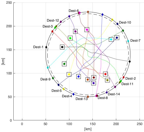
A Two-time-level Model for Mission and Flight Planning of
   an Inhomogeneous Fleet of Unmanned Aerial Vehicles
                                              a∗                               a
                       Johannes Schmidt                 Armin Fügenschuh

                                          March 18, 2021

                                              Abstract
            We consider the mission and flight planning problem for an inhomogeneous fleet
        of unmanned aerial vehicles (UAVs). Therein, the mission planning problem of as-
        signing targets to a fleet of UAVs and the flight planning problem of finding optimal
        flight trajectories between a given set of waypoints are combined into one model and
        solved simultaneously. Thus, trajectories of an inhomogeneous fleet of UAVs have to
        be specified such that the sum of waypoint-related scores is maximized, considering
        technical and environmental constraints. Several aspects of an existing basic model are
        expanded to achieve a more detailed solution. A two-level time grid approach is pre-
        sented to smooth the computed trajectories. The three-dimensional mission area can
        contain convex-shaped restricted airspaces and convex subareas where wind affects the
        flight trajectories. Furthermore, the flight dynamics are related to the mass change,
        due to fuel consumption, and the operating range of every UAV is altitude-dependent.
        A class of benchmark instances for collision avoidance is adapted and expanded to fit
        our model and we prove an upper bound on its objective value. Finally, the presented
        features and results are tested and discussed on several test instances using GUROBI
        as a state-of-the-art numerical solver.

Keywords: Mixed-Integer Nonlinear Programming, Mission Planning, Inhomogeneous
Fleet, Time Windows, Linearization Methods

1       Introduction
Due to their variety and flexibility, unmanned aerial vehicles (UAVs) have many possible
applications. Next to the long-studied military use [5], also many companies make efforts
to incorporate them into their processes, e.g., in parcel delivery [24], but for an efficient
and autonomous use, it is crucial to plan the considered task carefully since not only the
technical parameters of the used UAV but also the weather and maybe other airborne
UAVs must be taken into account. Furthermore, the mission area can contain airports,
power plants, or mountains, restricting the airspace and the possible routes. Incorporating
all these conditions into the planning process can make the resulting problem very intricate
to solve.
     The flight planning problem for a given number of inhomogeneous UAVs asks to calcu-
late a flight trajectory between a set of given waypoints for any considered UAV, complying
with its technical parameters and the related flight dynamics. The mission planning prob-
lem for an inhomogeneous fleet of UAVs is a version of the well-studied Vehicle Routing
Problem (VRP). Therein, a fleet of vehicles is assigned to a set of waypoints while the
    a
     Brandenburg University of Technology Cottbus-Senftenberg,
Platz der Deutschen Einheit 1, 03046 Cottbus, Germany,
{johannes.schmidt,fuegenschuh}@b-tu.de
   ∗
     Corresponding author

                                                   1
overall path should have minimal length. Next to the classical VRP, several of its vari-
ants are incorporating additional constraints, e.g., time windows or backhauls. Further
information about this problem class can be found in [27].
     We consider the mission and flight planning problem for an inhomogeneous fleet of
UAVs as a variant of the VRP with time windows, where further constraints regarding
the flight dynamics of the considered UAVs and the environment have to be taken into
account. UAVs do not rely on streets and can navigate through the air almost freely with
some related conditions like minimum velocity, maximum altitude, or restricted airspaces.
Furthermore, safety distances in aviation are stricter than in road traffic, where they are
negligible for modeling. Wind affects the flight of every UAV since their movement is
always relative to the surrounding atmosphere. Next to environmental parameters, the
mass of a flying object has a strong influence on its flight dynamics. Several characteristics,
e.g., maximum acceleration, maximum reachable altitude, or fuel consumption, depend on
it [23]. Finally, the operating range has to be observed if the connection of a UAV and its
ground control station is not a satellite link, but a UHF/VHF connection instead.
    In the literature, the mission planning problem for UAVs applies to a large number
of practical tasks, e.g., military operations [16], the observation of icebergs [1], or the
reconstruction of terrain from two-dimensional data [26], but often, the calculation of the
related flight trajectories is simplified or neglected.
    An extensive survey on the evolving field of civil applications for UAVs and possible
optimization approaches can be found in [19]. Due to the great interest in the autonomous
use of UAVs and the large number of related optimization approaches, we only highlight
some recent publications, where mission and flight planning is considered. Ramirez et
al. [20] use a genetic algorithm to assign several tasks to a fleet of inhomogeneous UAVs
considering technical parameters of the different types of UAVs, restricted airspaces, and
time windows. Zhen, Xing, and Gao [29] combine an ant colony algorithm for assigning
missions to a set of homogeneous UAVs with a Dubins curve to generate the trajectory
of every UAV. The resulting paths are affected by technical parameters of the consid-
ered UAV, collision avoidance constraints, and restricted airspaces. Ribeiro et al. [22]
use a mixed-integer linear program (MILP) to organize the observation of conveyor belts
in a mining site. Their approach is rather combinatorial without exact trajectories but
incorporates energy consumption and the possibility to place and use charging stations.
Li et al. [17] apply an ant colony algorithm combined with the metropolis criterion to
the problem of finding optimal trajectories for a fleet of homogeneous UAVs on a grid
map, regarding a given safety distance between the UAVs and given obstacles. Glock and
Meyer [10] present a neighborhood search algorithm to assign possible sampling locations
after fire or chemical incidents to a set of UAVs and plan their trajectories to maximize the
collected information in a given time horizon. Flight dynamics, i.e., maximum velocity,
acceleration, and battery level of the homogeneous fleet, are translated into travel times
between target locations. Coutinho, Fliege, and Battarra [6] formulate the problem of
surveying a set of locations in the aftermath of a disaster by pilotless gliders as a mixed-
integer nonlinear problem (MINLP). By applying several linearization techniques, they
achieve an MILP computing trajectories for several aircrafts from a starting point to a
set of possible landing areas within an obstacle-free airspace assuming constant weather
conditions. Cheng, Adulyasak, and Rousseau [4] derive a branch-and-cut algorithm to
solve an MINLP describing the problem of multi-trip parcel delivery by a homogeneous
fleet of UAVs. Considering constant altitude and velocity, their energy consumption is
modeled using a mass-dependent, nonlinear function, and trajectories are given by dis-
tances and travel times. Thibbotuwawa et al. [25] set up an MILP to plan the supply
of a set of customers with an inhomogeneous fleet of UAVs under weather uncertainty.
Their proposed model incorporates several weather zones, each with related wind con-

                                              2
ditions, energy consumption, and collision avoidance. In terms of the flight dynamics,
it lacks the exact trajectory, only computing the sequence of visited customers. Kai et
al. [14] give an MILP to plan the trajectory of a UAV visiting a given set of waypoints
taking into account detailed flight dynamics. In terms of environmental constraints, the
therein presented model lacks weather conditions and restricted airspaces. Xia, Wang,
and Wang [28] formulate the problem of controlling moving ships in emission control areas
by UAVs, stationed at the coast, as an MILP and compare it with a Lagrangian relax-
ation. The UAVs are assigned to computed waypoints, where they meet a vessel. Though,
besides the battery level, no flight dynamics are taken into account. Albert, Leira, and
Imsland [1] present an integer linear optimization model for the observation of drifting
icebergs in arctic areas to support shipping using a homogeneous fleet of UAVs deployed
at a ship. Their approach uses Dubins curves to compute trajectories and can update the
present path during the mission by a new run of the optimization model. But therefore,
it neglects most of the flight dynamics to speed up the solution process. Chen et al. [3]
consider a UAV as particle affected by different force fields and plan trajectories avoiding
given obstacles. The resulting problem is solved using optimal control theory but neglects
flight dynamics and weather conditions.
    Within the flight planning process, collision avoidance and conflict resolution is a
crucial field to ensure the safe operation of aircrafts and avoid significant harm. It considers
a given number of aircraft within the same airspace and asks for the best control changes
for each of them to achieve collision-free trajectories. If the problem is stated in three
dimensions, also altitude changes are possible to resolve conflicts. Although the process
of solving potential conflicts between midair aircraft is automated [15], considering this
aspect already in the operation planning phase can reduce the number of conflicts and
errors later.
    An extensive review about the field of conflict detection and resolution and related
solution methods can be found in [21]. Due to its currency, we further mention only
two forthcoming approaches. Dias, Rahme, and Rey [7] derive a two-stage algorithm
for conflict resolution using a mixed-integer quadratic and mixed-integer linear problem.
It computes collision-free linear trajectories for all aircrafts, while every aircraft reaches
its initial end position. Their model is tested on the class of benchmark instances that
we also adapt for our model. In [12], Hoch et al. consider collision avoidance as a non-
stop disjoint trajectory problem, where commodities are shipped through a time-expanded
graph without coming across each other. They study the general properties of this problem
and examine different graph classes which can be applied as takeoff/landing phase with
several aircraft or airspaces with a fixed number of airports and aircraft. Due to the
underlying network, this approach lacks detailed flight trajectories.
    We contribute to the state-of-the-art by considering the mission and flight planning
problem for an inhomogeneous fleet of UAVs in a mixed-integer non-linear programming
framework, including detailed flight dynamics of the different UAVs, the effect of wind in
different subareas and altitudes, convex shaped restricted airspaces, and collision avoid-
ance. Furthermore, we extend several of its aspects to enhance the quality of the computed
solution. The novelty of our approach is the combination of assigning waypoints to the
participating UAVs and calculating detailed flight trajectories at the same time. This pa-
per extends the work presented in [9]. The newly incorporated aspects are the following:
By the combination of two different time discretizations, the computed flight trajectories
have an increased level of detail. We incorporate mass-dependent maximum velocity, max-
imum acceleration, maximum reachable altitude, and a mass-dependent fuel consumption
into the presented model. The operating range of every UAV is defined dependent on
altitude, assuming no sky propagation, and the height of the used antenna. Restricted
airspaces are generalized to convex shaped areas and wind affects any UAV within spec-

                                               3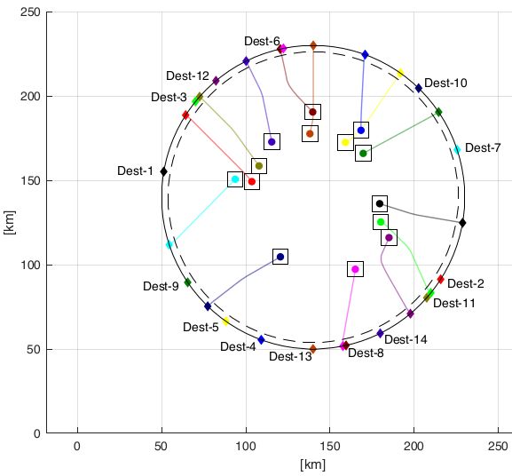
{0, n f + 1, 2 nf +1 , ... ,T nf +1 }=T
∆t
{ 0, 1, 2, .. , n f + 1,
... ,2 nf +1 , ... ∆t f ,T nf +1
} = Tf
Figure 1: Sets and time step lengths for the layers T and Tf of the two-level time grid
approach.
ified convex subareas. Considering collision avoidance, we adapt and extend a class of
benchmark problems to fit our model and derive upper bounds for their necessary amount
of discrete time steps in the two- and three-dimensional case.
This paper is structured as follows. In section 2, the basic model is set up by apply-
ing the two-level time discretization. Furthermore, the computation of the UAVs flight
dynamics, the operating range, the restricted airspaces, and the influence of wind are ex-
panded to allow more realistic constraints and achieve high-quality solutions. In section 3,
a class of benchmark instances for collision avoidance is adapted to the introduced model
and upper bounds for the necessary time horizon are given. The effect of the derived
modifications and results is tested in several scenarios in section 4, including the influence
of the time discretization on the computation time, comparison between the derived upper
bounds and the computed optimal solution for collision avoidance problems, and a detailed
discussion of particular aspects of our model. We summarize the presented results and
give directions for future work in section 5.
2 Two-level Time Model
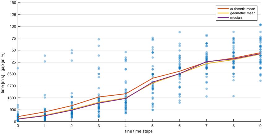
If the velocity and the acceleration can change only at any discrete time step, the step
length has to decrease to smoothen the computed trajectories. Thus, more time steps
are necessary to cover the same time interval, leading to more complex instances and
slower solution processes. In the following, we present a possibility to achieve smooth
trajectories by using two different, coupled time discretizations and apply it to the model
in [9]. Afterwards, the derived two-level time discretization model is extended in several
ways. A list of all used sets can be found in table 1. The parameters and variables within
the two-level time discretization model are given in tables 2 and 3, while the additional
parameters and variables of the complete extended model are described in tables 4 and 5.
The time horizon [0, ∆tT ], for a given number of time steps T and time step length ∆t,
is discretized in two different ways to achieve a better discretization without an increase in
the number of time steps and discrete decision variables. Let nf denote the number of fine
time steps between two adjacent time steps in T . For the first discretization, the step size
∆t is applied, but the set T contains all multiples of nf + 1 in the interval [0, (nf + 1)T ],
i.e., T = {0, nf + 1, . . . , (nf + 1)T }. This discretization is applied to the binary variables
to model the possible decisions. Second, each time step t ∈ {0, 1, . . . , T } is divided into nf
(fine) time steps, resulting in a step size ∆tf = nf∆t +1 and a set Tf = {0, 1, . . . , (nf + 1)T }.
This fine time approximation is applied to all continuous variables to refine the computed
trajectories. Furthermore, a function TtU : Tf → T of the form
t
TtU = (nf + 1) (1)
nf + 1
is necessary to map the fine time steps to their coarse counterpart, always rounding down.
As abbreviations T − = T \ {(nf + 1)T } and Tf− = Tf \ {(nf + 1)T } are used. Figure 1
holds an illustration of this two-level time grid approach. Using the two-level time grid
approach, the mission and flight planning problem for an inhomogeneous fleet of UAVs is
4Table 1: Overview of the sets used in the extended mission and flight planning model.
Symbol Index Definition
Lu i set of altitude bands of UAV u
L0,u = Lu ∪ {0} i set of altitude bands of UAV u including
the ground
P p set of all wind zones
Q q set of all restricted airspaces
T = {0, nf + 1, . . . , (nf + 1)T } t set of discrete time steps
T − = {0, nf + 1, . . . , (nf + 1)T − 1} t set of discrete time steps excluding the
last one
Tf = {0, 1, . . . , (nf + 1)T } t set of refined discrete time steps
Tf− = {0, 1, . . . , (nf + 1)T − 1} t set of refined discrete time steps exclud-
ing the last one
Tw ⊆ T t set of time steps at which waypoint w
can be visited
U u set of all considered UAVs
Vu j set of throttle bands of UAV u
W w set of all waypoints to be visited
given by
~0
~ru (0) = R ∀u ∈ U ,
u
(2.1)
~ru ((nf + 1)T ) = ~ T̃
R ∀u ∈ U ,
u
(2.2)
~ u k2 ≤ %u
k~ru (t) − G ∀u ∈ U , t ∈ Tf ,
(2.3)
hu bu (TtU) ≤ ruz (t) ≤ hu bu (TtU) ∀u ∈ U , t ∈ Tf ,
(2.4)
rui (t + 1) = rui (t) + ∆tf vui (t)
(∆tf )2 i
+ ∆tf wi (TtU)bu (TtU) + au (t) ∀u ∈ U , t ∈ Tf− , i ∈ {x, y},
2
(2.5)
vui (t + 1) = vui (t) + ∆tf aiu (t) ∀u ∈ U , t ∈ Tf− , i
∈ {x, y},
(2.6)
ruz (t + 1) = ruz (t) + ∆tf vuz,+ (t) − vuz,− (t) ∀u ∈ U , t ∈ Tf ,
(2.7)
v u (t)bu (TtU) ≤ k~vu (t)k2 ≤ v u (t)bu (TtU) ∀u ∈ U , t ∈ Tf ,
(2.8)
au (t)bu (TtU) ≥ k~au (t)k2 ∀u ∈ U , t ∈ Tf ,
(2.9)
5Table 2: Overview of the parameters used in the mission and flight planning model of
section 2.
Symbol Domain Definition
au R+ maximum acceleration of UAV u
~cq (t) R3 location of the top-right corner of restricted airspace q at time step
t
~cq (t) R3 location of the bottom-left corner of restricted airspace q at time
step t
Fu R+ maximum fuel of UAV u
~u
G R3 location of the ground control station for UAV u
Hu,i R+ altitude limit of UAV u in altitude band i
hu R+ maximum flight altitude of UAV u
hu 0, hu minimum flight altitude of UAV u
Mi R+ sufficiently large constants with different magnitude for i ∈
{dist, air, f uel, alt, vel}
nf N ∪ {0} number of fine time steps
p~w R3 location of waypoint w
R~0 R3 start location of UAV u
u
~
RuT̃ R3 end location of UAV u
Sw R+ score value for visiting waypoint w
v z,+
u R+ maximum climb rate of UAV u
v z,−
u R+ maximum descent rate of UAV u
vu R+ maximum velocity of UAV u
vu [0, v u ] minimum velocity of UAV u
w(t)
~ R2 horizontal wind velocity at time step t
T N number of coarse discrete time steps
∆t R+ length of one discrete time step
∆tf R+ length of one refined discrete time step
δu,w [0, %u ] maximum operational distance of UAV u to waypoint w
~ε R3+ required minimum safety distance between two UAVs
ηu,i,j R+ fuel consumption of UAV u in altitude band i and throttle band j
θu,j R+ velocity limit of UAV u in throttle band j
TtU T fine-to-coarse mapping for time discretization
ξu R+ fuel surplus of UAV u for climbing
%u R+ maximum operating range of UAV u
6Table 3: Overview of the variables used in the mission and flight planning model of
section 2.
Symbol Domain Definition
~au (t) R2 variable indicating the acceleration of UAV u at time step t in
horizontal direction
bu (t) {0, 1} binary variable indicating whether UAV u is airborne at time step
t
b+
u (t) {0, 1} binary variable indicating whether the task of UAV u started at
time step t or before
b−
u (t) {0, 1} binary variable indicating whether UAV u is still on its way at time
step t
du,w (t) {0, 1} binary variable indicating whether UAV u visits waypoint w at
time step t
~eu,u0 (t) {0, 1}3 binary variable indicating whether the distance between UAVs u, u0
is smaller than the safety distance in top-right direction
~eu,u0 (t) {0, 1}3 binary variable indicating whether the distance between UAVs u, u0
is smaller than the safety distance in bottom-left direction
f~u,q (t) {0, 1}3 binary variable indicating whether UAV u is below-left the top-
right corner of the restricted airspace q at time step t
f~u,q (t) {0, 1}3 binary variable indicating whether UAV u is upper-right the
bottom-left corner of the restricted airspace q at time step t
gu (t) R+ variable indicating the amount of remaining fuel of UAV u at time
step t
~ru (t) R3 variable indicating the position of UAV u at time step t
su,i,j (t) {0, 1} binary variable indicating whether UAV u is in altitude band i and
throttle band j at time step t
~vu (t) R2 variable indicating the horizontal velocity of UAV u at time step t
h i
vuz,+ (t) 0, v z,+
u variable indicating the climb rate of UAV u at time step t
h i
vuz,− (t) 0, v z,−
u variable indicating the descent rate of UAV u at time step t
7Table 4: Overview of the additional parameters introduced in sections 2.1 - 2.5.
Symbol Domain Definition
Au R+ height of the antenna at the ground control station of UAV u
C R+ sufficiently large constant
~cq,i (t) R3 normal vector of hyperplane i of restricted airspace q at time step
t
crhs
q,i (t) R right-hand side of the coordinate form related to hyperplane i of
restricted airspace q at time step t
E R+ radius of the earth
mu R+ empty weight of UAV u
NpP N number of hyperplanes describing wind zone p
NqQ N number of hyperplanes describing restricted airspace q
~np,i (t) R3 normal vector of hyperplane i of wind zone p at time step t
nrhs
p,i (t) R right-hand side of the coordinate form related to hyperplane i of
wind zone p at time step t
v z,+,0
u R+ maximum climb rate of UAV u at takeoff
v z,+
u,i,j R+ maximum climb rate of UAV u in altitude band i and throttle band
j
v z,−
u,i,j R+ maximum descend rate of UAV u in altitude band i and throttle
band j
v u,i R+ maximum velocity of UAV u in altitude band i
w
~ u,p,i (t) R3
w
~ l (t) R2 horizontal wind velocity in altitude band l at time step t
θu,i,j R+ velocity limit of UAV u in altitude band i and throttle band j
%alt R+ change of operating range per unit of altitude
%init R+ operating range on ground level
ϕacc
u R− obtainable percentage of the maximum velocity and acceleration
per unit of fuel for UAV u
ϕalt,1
u [0, 1) proportion of initial fuel for which UAV u can reach its maximum
altitude
ϕalt,2
u [0, 1) constant to set initial reachable altitude of UAV u
ϕfuuel R additional fuel consumption for every remainig unit of fuel of UAV
u
8Table 5: Overview of the additional variables introduced in sections 2.1 - 2.5.
Symbol Domain Definition
bu (t) {0, 1} binary variable indicating whether UAV u is airborne and has min-
imum velocity at time step t
fu,q,i (t) {0, 1} binary variable indicating whether UAV u is inside restricted
airspace q regarding hyperplane i at time step t
wu,p,i (t) {0, 1} binary variable indicating whether UAV u is inside wind zone p
regarding hyperplane i at time step t
wu,p (t) {0, 1} binary variable indicating whether UAV u is inside wind zone p at
time step t
−
bu (t) = b+
u (t) + bu (t) − 1 ∀u ∈ U , t ∈ T ,
(2.10)
b− −
u (t + 1) ≤ bu (t) ∀u ∈ U , t ∈ T − ,
(2.11)
b+ +
u (t) ≤ bu (t + 1) ∀u ∈ U , t ∈ T − ,
(2.12)
k~ru (t) − p~w k3 ≤ δu,w + M dist (1 − du,w (t)) ∀u ∈ U , w ∈ W, t ∈ T ,
(2.13)
X
du,w (t) ≤ 1 ∀w ∈ W,
u∈U ,t∈Tw
(2.14)
~cq (TtU) − M dist f~u,q (TtU) ≤ ~ru (t) ≤ ~cq (TtU) + M dist f~u,q (TtU) ∀u ∈ U , q ∈ Q, t ∈ Tf ,
(2.15)
~1 · f~ (t) + ~1 · f~u,q (t) ≤ 5 ∀u ∈ U , q ∈ Q, t ∈ T ,
u,q
(2.16)
0 0
~ru0 (t) + ε − M dist~eu,u0 (TtU) ≤ ~ru (t) ≤ ~ru0 (t) − ε + M dist~eu,u0 (TtU) ∀u, u ∈ U : u < u , t ∈ Tf ,
(2.17)
0 0
~1 · ~e 0 (t) + ~1 · ~e 0 (t) ≤ 7 − bu (t) − b 0 (t) ∀u, u ∈ U : u < u , t ∈ T ,
u,u u,u u
(2.18)
gu (0) = Fu ∀u ∈ U ,
(2.19)
gu (t + 1) = gu (t)
X
− ∆tf ξu vuz,+ + ηu,i,j su,i,j (TtU) ∀u ∈ U , t ∈ Tf− ,
i∈Lu ,j∈Vu
(2.20)
X
su,i,j (t) = bu (t) ∀u ∈ U , t ∈ T ,
i∈Lu ,j∈Vu
(2.21)
9!
X X
θu,j su,i,j (TtU) = k~vu (t)k2 ∀u ∈ U , t ∈ Tf ,
j∈Vu i∈Lu
(2.22)
X X X X
Hu,i−1 su,i,j (TtU) ≤ ruz (t) ≤ Hu,i su,i,j (TtU) ∀u ∈ U , t ∈ Tf .
i∈Lu j∈Vu i∈Lu j∈Vu
(2.23)
with the objective function
X 1 X t
max Sw du,w (t) − bu (t)
|Tf | M air
u∈U ,w∈W,t∈T u∈U ,t∈T
1 X gu (t) ruz (t) k~vu (t)k2
+ + − , (3)
|Tf | M f uel M alt M vel
u∈U ,t∈Tf
where k.k2 and k.k3 denote the two and three-dimensional Euclidean norm, respectively.
Constraints (2.1) and (2.2) fix the respective start and end location of every UAV, while (2.3)
limits their maximum operating range. The maximum and minimum altitude of the con-
sidered UAVs is restricted by (2.4). Equations (2.5) and (2.6) are a discretization of the
Newton’s equations of motion to compute the exact flight trajectory together with the
altitude changes in (2.7). The UAVs velocity and acceleration is bounded by (2.8) and
(2.9). In (2.10) – (2.12) it is ensured, that any UAV can only take off once and remain on
the ground after landing. The visit of the given waypoints is managed by (2.13) and (2.14),
guaranteeing that the respective UAV is inside the required operational range and every
waypoint is only visited once. Constraints (2.15) and (2.16) let a UAV avoid the given
restricted airspaces, while (2.17) and (2.18) manage the collision avoidance between any
pair of UAVs. The correct computation of the UAVs fuel consumption is ensured by
equations (2.19) – (2.23).
The presented model has to be linearized to achieve a mixed-integer linear problem.
We do this according to the methods shown in [9].
2.1 Flight Dynamics
In the given model, the left part of equation (2.8) forces every UAV to fly with at least
minimum velocity as soon as it takes off. If one of the deployed UAVs cannot accelerate
to its minimum velocity within a single time step, it would have to stay on the ground
and thus would not be used for mission planning. To overcome this drawback, we define
a new binary variable bu (t), indicating whether the minimum velocity has to hold.
l m
vu
Proposition 2.1. Let tu := (nf + 1) au ∆t for UAV u ∈ U . Then the equation
t+t
Xu
bu (t) ≥ bu (t0 ) − 2tu ∀u ∈ U , t ∈ {tu , (nf + 1)T − tu } (2.29)
t0 =t−t u
ensures bu (t) = 1 if and only if UAV u has minimum velocity.
Proof. Due to constraint (2.6), the UAVs velocity is a linear function of its acceleration.
Thus, the real time for reaching minimum velocity v u with maximum acceleration au is
v
given by auu . Conversion into a number discrete time steps tu ∈ N leads to
vu
tu := (nf + 1) . (4)
au ∆t
10Due to the objective function (3), the variable bu (t) is set to zero to save fuel, if this is
possible. To ensure that it is set to one tu time steps after the UAV starts to move or
before it attempts to land, we relate it to bu (t). Then,
bu (t) = 1 has to hold, if bu (t0 ) = 1
for all t ∈ {t − tu , t + tu }. To relate all 2 tu + 1 binary variables bu (t0 ) in this interval
0 0 0
to a single binary decision, 2tu is subtracted leading to the desired equation (2.29).
To incorporate the new variable, the minimum velocity has to hold only tu time steps
after takeoff. Thus, constraint (2.8) changes to
v u bu (TtU) ≤ k~vu (t)k2 ≤ v u bu (TtU) ∀u ∈ U , t ∈ Tf . (2.8’)
Accordingly, the fuel consumption equation (2.21) is adjusted to the new variable by
X
su,i,j (t) = bu (t) ∀u ∈ U , t ∈ T . (2.21’)
i∈Lu ,j∈Vu
Otherwise, equations (2.21) and (2.22) would force any UAV that cannot accelerate to its
minimum velocity in one timestep to stay on the ground.
Due to the physics of flight, a UAV slower than minimum velocity cannot ascend and
therefore not take off. Thus, similar to the minimum velocity, the left part of equation (2.4)
eliminates any UAV from the planning process if it cannot accelerate to its minimum
velocity and ascend to the minimum altitude within a single time step. To avoid this, the
variable bu (t) also is incorporated into equation (2.4), leading to
hu bu (TtU) ≤ ruz (t) ≤ hu bu (TtU) ∀u ∈ U , t ∈ Tf . (2.4’)
We consider the minimum altitude small enough such that any UAV with minimum ve-
locity can ascend to it within a fine time step.
Another occurring phenomenon in aviation is the altitude- and velocity-dependent
change of flight dynamics due to decreasing thrust in higher altitudes caused by decreasing
air temperature and pressure. It affects the maximum velocity as well as the maximum
climb and descent rates. For the maximum velocity, altitude dependence is incorporated
into the model by defining a maximum velocity v u,i of UAV u ∈ U for every of its altitude
bands i ∈ Lu and replace equation (2.8’) by
X X
v u bu (TtU) ≤ k~vu (t)k2 ≤ v u,i su,i,j (TtU) ∀u ∈ U , t ∈ Tf . (2.8’’)
i∈Lu j∈Vu
Besides this family of constraints, an altitude-dependent maximum velocity has to be
taken into account in the calculation of the fuel consumption. By redefining parameter
θu,j to θu,i,j , describing the velocity of UAV u ∈ U in throttle band j ∈ Vu and altitude
band i ∈ Lu , equation (2.22) changes to
X
θu,i,j su,i,j (TtU) = k~vu (t)k2 ∀u ∈ U , t ∈ Tf . (2.22’)
i∈Lu ,j∈Vu
For climb and descent rates, the velocity has to be taken into account, next to the altitude.
In a similar way to the velocity, the related parameters change to v z,+ z,−
u,i,j and v u,i,j , describing
the maximum climb and descent rate of UAV u ∈ U for altitude band i ∈ Lu and throttle
band j ∈ Vu , respectively. Thereby, the upper bounds for the variables vuz,+ (t) and vuz,− (t)
are no longer constant. Thus, the new constraint for the upper limit of the descent rate
is given by X
vuz,− (t) ≤ su,i,j (t)v z,−
u,i,j ∀u ∈ U , t ∈ Tf . (2.30)
i∈Lu ,j∈Vu
11For the climb rate, the approach is a bit different since a constraint similar to (2.30) would
reject any takeoff. Therefore, a new parameter v z,+,0
u is introduced for the maximum climb
rate at takeoff for every UAV u ∈ U and it is adjusted to get the maximum midair climb
rates v z,+
u . The constraint, limiting the climb rate for every UAV, then has the form
X
vuz,+ (t) ≤ v z,+,0
u − su,i,j (t) v z,+,0
u − v z,+
u,i,j ∀u ∈ U , t ∈ Tf . (2.31)
i∈Lu ,j∈Vu
In model (2), the maximum acceleration of the UAVs is assumed to be constant in every
situation. Thus, the computed flight trajectories are inaccurate since in practice the
maximally allowed acceleration at the takeoff is significantly higher than during the flight.
This results either in underestimation during the takeoff phase or overestimation when
in midair. We follow the approach given in the Base of Aircraft Data [18] (BADA) of
the Eurocontrol Experimental Centre. Therein, a reduction factor from takeoff thrust to
cruise thrust applies with a value of CT cr = 0.95. It is incorporated into the model by
changing equation (2.9) to
au (t) bu (TtU) − 0.05bu (TtU) ≥ k~au (t)k2 ∀u ∈ U , t ∈ Tf . (2.9’)
2.2 Fuel-dependent Flight Dynamics
The flight dynamics in model (2) are independent of the mass of the considered UAVs,
but this assumption only holds for electrical systems, where the weight of the battery is
constant. For UAVs with liquid fuels, the mass affects the maximum velocity, maximum
acceleration, maximum altitude, and fuel consumption rate [23] of an aircraft by weight
reduction due to burned fuel. Since the portion of the fuel on the gross take-off weight of
a UAV can go up to 43% [8], this has a great impact on the mission planning scenario.
To include these fuel-dependent flight dynamics into the proposed model, several changes
are necessary.
In terms of the altitude, we assume a linear dependency between the amount of re-
maining fuel and the reachable altitude. We expect the empty weight mu of UAV u to
include a small fuel reserve. Let UAV u ∈ U reach altitude hu 1 − mguu+F(0)
u
for an initial
amount of fuel gu (0) and its maximum altitude hu for ϕalt,1 u gu (0), with ϕalt,1
u ∈ [0, 1).
Additionally, there is an additive constant ϕalt,2
u ∈ [0, 1] to achieve a more flexible inital
altitude. The resulting linear function is displayed in figure 2 and gives the cosntraint
alt,1
ϕ u gu (0) − gu (t)
ruz (t) ≤ hu 1 + ϕalt,2
u + ∀u ∈ U , t ∈ Tf . (2.32)
alt,1
1 − ϕu (mu + Fu )
Besides, the right part of constraint (2.4’) is still necessary to limit the reachable altitude
to its maximum value and set the maximum altitude to zero when the UAV is on the
ground.
To include the mass of the remaining fuel into the calculation of the velocity and the
acceleration, we have the following proposition.
Proposition 2.2. For any UAV u ∈ U and time step t ∈ Tf , the linear approximations
X
gu (t)
k~vu (t)k2 ≤ ϕacc
u + 1 v u,i + V u 1 − su,i,j (TtU)
Fu + m u
j∈Vu
∀i ∈ Lu (2.33)
12hu
ϕalt,2
u hu
g0
hu 1 − Fu +mu
ϕualt,1 gu (0) gu (0)
Figure 2: Linear dependency between the amount of fuel and the reachable altitude.
and
gu (t)
k~au (t)k2 ≤ ϕacc
u + 1 au , (2.34)
Fu + m u
with V u = maxi∈Lu v u,i and
p
2 (Fu − 2mu ) m2u + Fu mu + 2m2u − 32 Fu2
ϕacc
u = (mu + Fu ) , (5)
Fu3
minimizes the quadratic error of the mass-dependent maximum velocity and acceleration,
respectively.
Proof. We compare the given maximum velocity v u related to mu with another velocity ṽu
for a UAV with more remaining fuel. Since the generated thrust of UAV u ∈ U is limited,
it can reach a certain kinetic energy Eumax = 21 mu v 2u for a given time. Thus, by energy
preservation, we get the relation
r
1 1 mu
(mu + gu (t))ṽu2 = mu v 2u ⇒ ṽu = vu. (6)
2 2 mu + gu (t)
Using the equation a = vt , in the same way the expression
r
mu
ãu = au (7)
mu + gu (t)
can be derived. Since we consider the maximum velocity and acceleration in (6) and (7),
we restrict on the positive solution of the respective square root. The non-linear factor
for equations (6) and (7) is the same. Thus, we only have to perform one least squares
approximation of the form
Z Fu r 2
mu acc gu (t)
min − ϕu +1 dgu (t), (8)
acc
ϕu 0 mu + gu (t) mu + Fu
where we fix the absolute term of the linear function to 1 to ensure that the maximum
1
velocity and acceleration is attained according to tour assumption. The factor mu +F u
acc
is applied to have a greater numerical value for ϕu and thus avoid numerical issues.
The solution of (8) gives the desired parameter ϕacc u for the obtainable percentage of
the maximum velocity and acceleration per unit of fuel for UAV u ∈ U . Replacing the
gu (t)
factor bu (TtU) − 0.05bu (TtU) by the computed linear function ϕacc
u Fu +mu + 1 in (2.9’), it
13gives the desired mass-dependent maximum acceleration (2.34) for every airborne UAV
u ∈ U in time step t ∈ Tf . In terms of the mass-depedent maximum velocity, the above
approach is used and slightly modified since the altitude dependence
in (2.8’’) calls
for
P
the incorporation of an sufficiently large additive constant V u 1 − j∈Vu su,i,j (TtU) with
V u = maxi∈Lu v u,i to avoid nonlinearities. This leads to the remaining equation (2.33).
In addition to equations (2.33) and (2.34) the constraints (2.8’’) and (2.9’) are still
necessary to force the maximum velocity and acceleration to zero for grounded UAVs. The
used approach is similar to the method in the BADA [18], except that we assume the UAV
to reach maximum velocity and acceleration with only the fuel reserve incorporated in the
empty weight. In terms of the fuel-dependent fuel consumption, a further parameter ϕfuuel
is necessary. It describes the additional fuel consumption for every remaining fuel unit at
the previous time step and is incorporated as an additional factor into the constraint (2.20).
To ensure that a UAV is consuming no fuel when landed, a distinction between the fuel
calculation for a landed and a flying UAV is needed. Thus, the constraint (2.20) is replaced
by
gu (t + 1) ≤ Fu (1 − bu (TtU)) + gu (t)
X
− ∆tf ξu vuz,+ + ηu,i,j su,i,j (TtU) + ϕfuuel gu (t) ∀ u ∈ U , t ∈ Tf− , (2.20i)
i∈Lu ,j∈Vu
gu (t + 1) ≥ −Fu (1 − bu (TtU)) + gu (t)
X
− ∆tf ξu vuz,+ + ηu,i,j su,i,j (TtU) + ϕfuuel gu (t) ∀ u ∈ U , t ∈ Tf− , (2.20ii)
i∈Lu ,j∈Vu
gu (t + 1) ≤ gu (t) + Fu bu (TtU) ∀ u ∈ U , t ∈ Tf− , (2.20iii)
gu (t + 1) ≥ gu (t) − Fu bu (TtU) ∀ u ∈ U, t ∈ Tf− . (2.20iv)
Applying these changes to the model, the flight dynamics of the UAVs are compromised
since equation (2.19) ensures that every UAV takes off with maximum fuel, reducing the
maximum altitude, velocity, and acceleration. Thus, equation (2.19) is dropped to make
the amount of takeoff fuel variable and allow the UAVs to reduce the amount of initial
fuel to achieve better flight dynamics. To ensure these fuel-saving aspects, the objective
function (3) has to change to
X 1 X gu (0) 1 X t
max Sw du,w (t) − − bu (t)
|U| M f uel Fu T M air
u∈U ,w∈W,t∈T u∈U u∈U ,t∈T
1 X rz (t) k~vu (t)k2
u
+ − . (3’)
|Tf | M alt M vel
u∈U ,t∈Tf
2.3 Range
In model (2), the maximum operating range %u is chosen constant, although it depends
on the height Au of the used antenna and the altitude ruz (t) of the UAV. To achieve more
a realistic setting, we deduce an altitude-dependent maximum range.
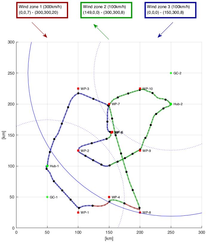
Proposition 2.3. Let C be a constant with C ≥ maxu∈U hu . Then the linear approxima-
tion
~ u k2 ≤ %alt rz (t) + %̃init ,
k~ru (t) − G (2.3’)
u
14Au
%u
ruz (t)
E
Figure 3: Maximal operating range %u of a UAV for antenna height Au and altitude ruz (t).
p
with %̃init = %init + 2Au E − A2u and coefficients %alt , %init solving
2C 3 alt 2 init 3 π −1 E−C
E−C q
E−C 2
3 % + C % = E 2 − sin E − E 1− E ,
3
2 32
− 2E3 1 − E−C (9)
E
2 alt init 2 π −1 E−C
E−C q
E−C 2
C % + 2C% = E 2 − sin E − E 1− E ,
minimizes the quadratic error to the altitude-dependent maximum operating range at time
step t ∈ Tf .
Proof. The maximum range of UAV u ∈ U can be displayed as in figure 3. Applying the
Pythagorean theorem, the maximum range is calculated by
p p
%u (ruz (t)) = 2Au E − A2u + 2Eruz (t) − (ruz (t))2 , u ∈ U , t ∈ Tf , (10)
where E is the radius of the earth and Au is the height of the antenna.
Due to the nonlinearity of this expression, we use the continuous least squares method
to find the best approximation in terms of a linear function f (x) = %alt x + %init . Since
the antenna height Au is constant, the first term in (10) is an additive constant and only
shifts the whole function. Thus it can be neglected in the least squares approximation,
leading to the problem
Z C p 2
min 2Eru (t) − (ru (t)) − (% ru (t) + % ) druz (t),
z z 2 alt z init
(11)
˜
%alt ,%init 0
with C ≥ maxu∈U hu representing a sufficiently large altitude as upper limit of the integral.
By integration and solution of the remaining minimization problem, the parameters %alt
and %init are given by (9). Finally, the constant maximum operating range %u in (2.3) is
replaced by the linear function %alt ruz (t) + %̃init to obtain (2.3’).
2.4 Restricted Airspaces
Equations (2.15) and (2.16) in model (2) allow to incorporate restricted airspaces for the
UAVs, but only cubic ones which are parallel to the coordinate axes. To compare the
respective coordinates of UAV u ∈ U and the restricted airspace q ∈ Q at time step t ∈ T
i
and report if it is inside the area, two binary variables f iu,q f u,q are necessary for every
15coordinate direction i ∈ {x, y, z}, one per side. Using this approach, also more complex
restricted airspaces can be modeled by a union of these cubic ones, but only at the expense
of many additional binary variables.
To describe restricted airspaces by arbitrary polyhedrons, we assume its NqQ describing
hyperplanes to have coordinate form with normal vector ~cq,i (t) and right-hand side crhs
q,i (t)
Q
for i = 1, . . . , Nq and q ∈ Q. Thus, every restricted airspace q ∈ Q is represented by
n o
Q 3 rhs Q
Aq (t) = ~x ∈ R |~cq,i (TtU) · ~x ≤ cq,i (TtU), i = 1, . . . , Nq . (12)
Similar to the parameters, the related binary variables f (t) are redefined to fu,q,i (t), with
fu,q,i (t) = 1 if UAV u ∈ U is outside of the restricted airspace q ∈ Q regarding hyperplane
i = 1, . . . , NqQ at time step t ∈ T , and fu,q,i (t) = 0 otherwise. Then equations (2.15) and
(2.16) are replaced by
~cq,i (TtU) · ~ru (t) ≥ crhs
q,i (TtU) − M
dist
(1 − fu,q,i (TtU))
∀u ∈ U , q ∈ Q, i = 1, . . . , NqQ , t ∈ Tf , (2.15’)
NqQ
X
fu,q,i (t) ≥ 1 ∀u ∈ U , q ∈ Q, t ∈ T , (2.16’)
i=1
providing a more general approach to model restricted convex airspaces with again one
binary variable per side.
2.5 Wind
In the basic model (2), the wind is assumed to blow constantly everywhere within the
considered area. By introducing the fine time steps, the wind can change in every fine
time step t ∈ Tf . To allow a more accurate influence of weather conditions, we want to
include the possibility of different wind zones within the mission area. But this comes with
the restriction that wind changes only in time steps t ∈ T . For simplicity, the computation
of the position (2.5) is modified to
(∆tf )2 i
rui (t + 1) = rui (t) + ∆tf vui (t) + w̃ui (t) + au (t)
2
∀u ∈ U , t ∈ Tf− , i ∈ {x, y}, (2.5’)
where w̃ui (t) is the influence of wind for UAV u ∈ U in coordinate direction i ∈ {x, y} at
time step t ∈ Tf− .
As a first approach, altitude-dependent wind zones could be added since the wind
intensity and its direction can change with increasing altitude, e.g., the jetstream has to
be taken into account for mission planning in altitudes between 8 to 12 2kilometers. To
x y
incorporate this into our model, the wind vector w~ l (t) = wl (t), wl (t) ∈ R is now defined
for every altitude band l ∈ Lu . Since the variable su,i,j (t) cannot change in every fine step,
there is a discretization error between two time steps if the altitude layer is changed. To
reduce its influence, we consider a convex combination of the wind between time steps
t, t + nf + 1 ∈ T at every fine time step t ∈ Tf . Thus, the influence of wind is calculated
by
X
w̃ui (t) = (1 − µ) wli (TtU)su,i,j (TtU) + µwli (VtW)su,i,j (VtW)
l∈Lu ,j∈Vu
∀u ∈ U , t ∈ Tf− , i ∈ {x, y}, (13)
16t mod (n +1)
f
with µ = nf +1 and VtW = TtU + nf + 1. But this method requires again constant
wind direction within every altitude band over the whole mission area.
To overcome this drawback, a second approach is possible. In the same way as for
the restricted airspaces in section 2.4, a set P of wind zones is defined, described by NpP
hyperplanes
n o
APp (t) = ~x ∈ R3 |~np,i (TtU) · ~x ≤ nrhs P
p,i (TtU), i = 1, . . . , Np , (14)
with normal vectors ~np,i (t) and right-hand sides nrhs
p,i (t).
Furthermore, new binary variables wu,p,i (t) ∈ {0, 1} are introduced with wu,p,i (t) = 1,
if UAV u ∈ U is within wind zone p ∈ P regarding hyperplane i ∈ APp at time step t ∈ T .
In contrast to the restricted airspaces, now additional constraints and an auxiliary binary
variable ωu,p (t) are necessary to map the variables wu,p,i (t) to a single binary decision and
to ensure that wind is only taken into account when UAV u ∈ U is in midair. Therefore,
the decision if UAV u is affected by wind zone p at time step t is modeled by
~nu,p,i (TtU) · ~ru (t) ≥ nrhs
p,i (TtU) − M
dist
wu,p,i (TtU)
∀u ∈ U , p ∈ P, i = 1, . . . , NpP , t ∈ Tf , (2.35)
NpP
X
wu,p,i (t) ≤ NpP + ωu,p (t) − 1 ∀u ∈ U , p ∈ P, t ∈ T , (2.36)
i=1
NP
X
p
wu,p,i (t) ≥ NpP ωu,p (t) ∀u ∈ U , p ∈ P, t ∈ T , (2.37)
i=1
X
ωu,p (t) ≤ |P|bu (t) ∀u ∈ U , t ∈ T . (2.38)
p∈P
Analogue to the first approach, the variable wu,p (t) can only change at time step t ∈ T .
Thus, the convex combination with t̃ is applied again and the influence of wind is calculated
by
X
w̃ui (t) = (1 − µ) wpi (TtU)ωu,p (TtU) + µwpi (VtW)ωu,p (VtW)
p∈P
∀ u ∈ U , t ∈ Tf− , i ∈ {x, y}, (2.39)
t mod (nf +1)
where again µ = and VtW = TtU + nf + 1. For this approach, the number of
nf +1
P
binary variables within the model increases by p∈P (|APp | + 1) per time step and UAV.
3 Collision Avoidance
Compliance with safety distances in aviation is crucial due to the disastrous consequences
of its failure. Therefore, the parts of a planning model computing collision-free flight tra-
jectories should be examined excessively. In the following, we consider a two dimensional
and a three dimensional setting to examine the modelled collision avoidance (2.17) and
(2.18).
A class of two-dimensional benchmark instances, called Random Circle Problems
(RCPs) [7], has a wide application in collision avoidance and conflict resolution. In this
problem class, a set of aircrafts is randomly arranged on a circle. At the beginning, all
UAVs maintain the safety distances, head towards the circles center, and have their re-
spective destination on its opposite side. The deviation from the shortest connection is
17minimized for every participant. With an increasing number of aircrafts, it is a challenging
problem to conflict resolution approaches due to its fast increasing violations of the safety
distance if no countermeasures are taken.
We adapt these benchmark instances to our setting, assuming every participating UAV
has the same technical characteristics. Thus, there are no waypoints and the start locations
of the participating UAVs are distributed randomly along a circle of radius rRCP , with
their respective end location on the opposite side. The operating range is neglected since
every UAV must be able to reach its end location. Thus, the whole circle is within its
operating range. In the beginning, every UAV is heading towards the center of the circle
and all safety distances are ensured. To incorporate this into the model, a new constraint
vu (0) = γu · ~1 · C~ −R
~0 ∀u ∈ U , (15)
u
is added, where C ~ is the location of the center of the considered circle and the new variable
γu scales the given direction to ensure the limits of the velocity.
Due to the absence of waypoints and the altitude, many constraints can be neglected
and also many binary variables are unnecessary or must be redefined, i.e., su,i,j (t) changes
to su,j (t) indicating whether UAV u ∈ U is within throttle band j ∈ V1 at time step t ∈ T
and the variables bu (t) and bu (t) are substituted by b− u (t) since all UAVs start in midair
and have to stop at their end location.
We minimize the deviation of the shortest connection by the number of necessary time
steps T min , such that every UAV reaches its respective end location. This number is not
known a priori and increases the more UAVs are participating. Only a lower bound T min
is given by the number of time steps it takes for a single UAV to fly along the diameter
of the circle with maximum velocity. Setting T to a sufficiently large value and read
T min from the optimal solution can be an ineffective way since the number of constraints
and variables is time-dependent, leading to a possibly too large model. Therefore, we
use an approach from [2], solving the RCP sequentially for an increasing number of time
steps, starting with T = T min , until a feasible solution is found or its existence cannot
be determined within a given computation time. This procedure has the advantage of
working without any objective function since the first found feasible solution gives the
value of T min .
To ensure that the safety distances are observed at every time step, it has to hold
maxi∈{x,y} εi
∆t ≤ , (16)
V1
where V 1 = maxi∈L1 v 1,i is again the maximum of the altitude-dependent maximum ve-
locities of the first UAV. Due to the assumption of identical technical characteristics of
all participating UAVs, the first UAV can be chosen without loss of generality. Without
condition (16), a pair of UAVs, complying with the safety distance between them, could
swap their positions within one time step by flying through each other. The resulting
resolution of the time is sufficient to obtain smooth trajectories. Thus, we renounce on
fine time steps in this case.
The following result gives a heuristical solution for the two-dimensional RCP.
Proposition 3.1. Consider the two-dimensional RCP with center C ~ ∈ R2 , radius rRCP ∈
2
R+ , safety distances ~ε ∈ R+ , time step length ∆t ∈ R+ , n ∈ N participating UAVs, and
v ∈ R+ their maximum velocity. Then it holds
& '
2rRCP + (π − 2)kC~ − ~rn (t0 )k
min
T ≤ , (17)
v∆t
18with
t0 = min {k~ru1 (t + 1) − ~ru2 (t + 1)k ≤ k~εk | u1 , u2 ∈ {1, . . . , n}; u1 < u2 } . (18)
t∈Z+
Proof. Every UAV starts at its random starting location and heads towards the center C ~
~
with maximum speed. To avoid conflicts near the center C, all UAVs are assigned to a
smaller circle with center C~ and radius rub ≤ rRCP before the first conflict would occur.
Along this smaller circle, the UAVs rotate around its center on a semicircle and then fly
to their respective end locations. This approach generates a feasible solution if the safety
distances are observed during the rotation. Therefore, it is necessary to ensure at least the
distance k~εk between any pair of UAVs. Let t0 be the last time step with this property. It
is be computed by
t0 = min {k~ru1 (t + 1) − ~ru2 (t + 1)k ≤ k~εk | u1 , u2 ∈ {1, . . . , n}; u1 < u2 } . (19)
t∈Z+
~ −~rn (t0 )k, where the position of any UAV at time step t0
The radius rub is then given by kC
can be chosen since they all have equal distance to the center. Without loss of generality,
we take the position of UAV n. For the described solution, every UAV must fly a distance
of 2(rRCP − rub ) + πrub units to reach its end location. Thus, there are
2rRCP + (π − 2)rub
T = (20)
v∆t
time steps necessary to complete this trajectory. Substitution of rub leads to the upper
bound of T min given in (17).
Furthermore, the quality of the described heuristic solution can be calculated.
Corollary 3.2. For the two-dimensional RCP with minimum number of time steps T min ,
it holds
T min π
1 ≤ min ≤ . (21)
T 2
Proof. In the worst case, there are two UAVs u1 , u2 ∈ U starting with kR ~ 0 k = k~εk.
~ u0 − R u2
1
Then it follows rub = rRCP and the trajectory of every UAV is πrRCP . Since all UAVs
have the same constant maximum velocity v, it holds T min = 2rRCP v and the number of
time steps T min depends only on the radius rRCP , leading to T min = πrRCP v = π2 T min .
Thus, in a general setting the desired estimate (21) is obtained by combining the definition
of T min with the described worst case and rearranging it.
For the case of evenly distributed UAVs, the result of proposition 3.1 can be computed
without the knowledge of t0 .
Corollary 3.3. Consider the Circle Problem with n ∈ N evenly distributed UAVs with
maximum velocity v ∈ R+ , radius rRCP ∈ R+ , safety distances ~ε ∈ R2+ , and time step
length ∆t ∈ R+ . Then it holds
(π−2)
2rRCP + π k~
2 sin( n
εk
)
T min ≤
.
(22)
v∆t
Proof. In the evenly distributed case, every pair of UAVs has the same distance. Thus,
their start locations are the corners of a regular polygon with circumradius rRCP . Since all
UAVs head towards the center with the same velocity, they stay corner points of a regular
19polyhedron with decreasing side length. The radius rub of the smaller circle is then the
circumradius of a regular polyhedron with n corners and side length ~ε. It is computed by
k~εk
rub = (23)
2 sin πn
Substituting this term into (20) gives the upper bound (22).
The model in the two-dimensional case is given by the constraints (2.1), (2.2), (2.5’),
(2.6), (2.8’), (2.9’), (2.11), (2.17), (2.18), (2.20i) – (2.20iv), (2.21), (2.22), (2.33), (2.34),
and (15), where all terms with vuz,+ (t) are neglected, due to the absence of altitude changes.
Furthermore, the variables bu (t) and bu (t) have to be substituted by b− u (t) since all UAVs
start in midair and should only stop at their respective end locations.
Since in ordinary air traffic the aircrafts are not restricted to a single altitude and
to fully evolve the potential of our model, we extend the concept of RCPs into three
dimensions. Therefore, minimum and maximum altitudes h and h are incorporated as
lower and upper bound of the altitude ruz (t) of every UAV u ∈ U at time step t ∈ Tf ,
respectively. All UAVs are positioned analog to the two-dimensional case, but with initial
altitude R0,z ∈ h, h .
The result of proposition 3.1 can also be adapted for the three-dimensional RCP.
~ ∈ R3 , radius rRCP ∈
Proposition 3.4. Consider the three-dimensional RCP with center C
R+ , minimum and maximum altitude h and h, safety distances ~ε ∈ R3+ , and time step
length ∆t ∈ R+ . Let nl = b h−h εz c and the sets U1 , . . . , Unl be a partition of U = {1, . . . , n}.
Furthermore, every participating UAV has maximum velocity v ∈ R+ , maximum climb
and descent rate v z,+ and v z,− , and initial altitude R0,z . Then it holds
(& '
2rRCP + (π − 2)kC~ − ~rn (t0 )k |R0,z − h + (i − 1)εz |
min i
T ≤ max +
i∈{1,...,nl } v∆t v z,+ ∆t
0,z )
|R − h + (i − 1)εz |
+ , (24)
v z,− ∆t
with
t0i = min {k~ru1 (t + 1) − ~ru2 (t + 1)k ≤ k~εk | u1 , u2 ∈ Ui ; u1 < u2 }
t∈Z+
∀i ∈ {1, . . . , n}. (25)
Proof. For the given altitude range h, h and vertical safety distance εz , it is possible to
stack nl = b h−h εz c UAVs one above each other at the same x- and y-coordinates. Thus,
every partition {Ui }i∈{1,...,nl } of the set U = {1, . . . , n} decomposes the three-dimensional
RCP into nl two-dimensional RCPs considering only the UAVs Ui , respectively. According
to this, the number of time steps to perform the three-dimensional trajectory of every UAV
u is the sum of the number of time steps for its trajectory in the two-dimensional problem
and the number of time steps necessary for the altitude changes.
To arrange all two-dimensional RPCs into the altitude range h, h , one of them is
located at the lower or upper altitude limit and the vertical distance between two of them
is at least εz . Without loss of generality, we assign the problem considering the UAVs of
subset U1 to the altitude h. Then, the necessary number of time steps for the altitude
changes of every UAV u ∈ Ui are computed by
0,z 0,z
z |R − h + (i − 1)εz | |R − h + (i − 1)εz |
Ti = + ∀i ∈ {1, . . . , nl }. (26)
v z,+ ∆t v z,− ∆t
20Table 6: Data for the UAV technical parameters according to [8].
Description Parameter Unit UAV-1 UAV-2
km
Minimum velocity vu h 130 167
km
Maximum velocity vu h 232 204
Military static thrust at s/l FuN kp 1250 64
Maximum initial climb rate v z,+,0
u
m
s 8 2
Maximum fuel Fu kg 2000 150
kg
Fuel surplus for climbing ξu min 0.2 0.02
Empty weight mu kg 4000 540
Thus, the number of necessary time steps in the three-dimensional case is computed by
& '
~ − ~rn (t0 )k
2rRCP + (π − 2)kC |R0,z − h + (i − 1)εz |
Ti = +
v∆t v z,+ ∆t
0,z
|R − h + (i − 1)εz |
+ ∀i ∈ {1, . . . , nl }, (27)
v z,− ∆t
with t0 from proposition 3.1. The maximum of these Ti is the desired upper bound (24).
The model in the two-dimensional case is given by the constraints (2.1), (2.2), (2.5’) –
(2.9’), (2.11), (2.17), (2.18), (2.20i) – (2.20iv), (2.21) – (2.23), (2.30), (2.31), (2.33), (2.34),
(15), and the constraint
h ≤ ruz (t) ≤ h ∀u ∈ U , t ∈ Tf . (28)
Similar to the two-dimensional case, the variables bu (t) and bu (t) are substituted by b−
u (t).
4 Computational Results
To test the derived results, we apply the extended model (2) with objective (3’) to different
instances considering real-world UAVs. These are:
UAV-1. Heron TP UAV [Eitan] - Israel (Air Force), since 2012.
UAV-2. RQ-5A Hunter UAV - United States (Army), since 1996.
The data for the technical parameters of the UAVs are taken from [8] and can be found
in Table 6 to Table 8.
As length of one time step, ∆t = 0.1h is assumed. Regarding the maximum operating
range, we choose in (9) C range = 15km, E = 6371km, and Au = 0.005km for all u ∈ U
. Thus, we obtain the optimal values m := 23.30 and ñ := 116.61, leading to the linear
approximation displayed in figure 4. For the altitude and throttle dependend climb rate
we assume v z,+ z,+,0
u,i,j = v u for all UAVs u ∈ U , altitude bands i ∈ Lu , and throttle bands
j ∈ Vu .
The operational range δu,w of UAV u ∈ U to waypoint w ∈ W is set to a value within
the second highest altitude band to reject the UAVs staying at maximium altitude all the
time. According to this, we choose the values δ1,w = 10km and δ2,w = 3km.
21Table 7: Altitude and throttle band related data of UAV-1 according to [8].
Altitude- Altitude velocity descend rate fuel cons.
km m kg
Throttle band (in km) (in h ) (in s) (in min )
Altitude band 1 0.001– 3.658 130 8 2.08
loiter speed
Altitude band 1 0.001– 3.658 204 24 2.60
cruise speed
Altitude band 1 0.001– 3.658 232 24 5.23
military speed
Altitude band 2 3.658– 7.315 130 8 1.53
loiter speed
Altitude band 2 3.658– 7.315 204 24 1.91
cruise speed
Altitude band 2 3.658– 7.315 232 24 3.85
military speed
Altitude band 3 7.315– 10.972 130 8 1.06
loiter speed
Altitude band 3 7.315– 10.972 204 24 1.33
cruise speed
Altitude band 3 7.315– 10.972 232 24 2.66
military speed
Altitude band 4 10.972– 13.716 130 8 0.70
loiter speed
Altitude band 4 10.972– 13.716 204 24 0.88
cruise speed
Altitude band 4 10.972– 13.716 232 24 1.78
military speed
22You can also read