Cognitive prediction of obstacle's movement for reinforcement learning pedestrian interacting model
←
→
Page content transcription
If your browser does not render page correctly, please read the page content below

Journal of Intelligent Systems 2022; 31: 127–147 Research Article Thanh-Trung Trinh* and Masaomi Kimura Cognitive prediction of obstacle's movement for reinforcement learning pedestrian interacting model https://doi.org/10.1515/jisys-2022-0002 received February 19, 2021; accepted October 31, 2021 Abstract: Recent studies in pedestrian simulation have been able to construct a highly realistic navigation behaviour in many circumstances. However, when replicating the close interactions between pedestrians, the replicated behaviour is often unnatural and lacks human likeness. One of the possible reasons is that the current models often ignore the cognitive factors in the human thinking process. Another reason is that many models try to approach the problem by optimising certain objectives. On the other hand, in real life, humans do not always take the most optimised decisions, particularly when interacting with other people. To improve the navigation behaviour in this circumstance, we proposed a pedestrian interacting model using reinforcement learning. Additionally, a novel cognitive prediction model, inspired by the predictive system of human cognition, is also incorporated. This helps the pedestrian agent in our model to learn to interact and predict the movement in a similar practice as humans. In our experimental results, when compared to other models, the path taken by our model’s agent is not the most optimised in certain aspects like path lengths, time taken and collisions. However, our model is able to demonstrate a more natural and human-like navigation behaviour, particularly in complex interaction settings. Keywords: agent, cognitive prediction, navigation, pedestrian, reinforcement learning MSC 2020: 68T42, 68U99, 91E10 1 Introduction Constructing a human-like pedestrian navigation model is a problem that requires much attention from many research fields. The studies in the robotics domain, for example, are required to address this problem to build robots that are capable of manoeuvring in real-world environments [1–3]. Another example is the studies in urban planning, in which the pedestrian navigation behaviour needs to be constructed to analyse the possible activities of the people moving in the area [4,5]. Consequently, potential risks could be early detected and eliminated to ensure the necessary safety precautions for an infrastructure project. Different approaches have been considered to address this problem. The majority of these are physics-based, such as using forces [6] or fluid dynamics [7], to realise the pedestrian’s movement. Other approaches replicate the pedestrian behaviour by using rule-based models [8] or more recently, using neural networks [9]. They usually aim at optimising certain objectives, such as shortest path or minimising the number of collisions. These approaches are sufficient to simulate common pedestrian situations as well as in certain scenarios like evacuation or traffic congestion. * Corresponding author: Thanh-Trung Trinh, Graduate School of Engineering and Science, Shibaura Institute of Technology, Koto City, Tokyo 135-8548, Japan, e-mail: nb18503@shibaura-it.ac.jp Masaomi Kimura: Department of Computer Science and Engineering, Shibaura Institute of Technology, Koto City, Tokyo 135-8548, Japan, e-mail: masaomi@shibaura-it.ac.jp Open Access. © 2022 Thanh-Trung Trinh and Masaomi Kimura, published by De Gruyter. This work is licensed under the Creative Commons Attribution 4.0 International License.
128 Thanh-Trung Trinh and Masaomi Kimura
However, when replicating the close interaction between pedestrians, for example, when the pedes-
trian needs to avoid another person who suddenly changes his direction, these models often create unreal-
istic behaviour. There are two possible reasons for that. First, these models often ignore the cognitive
factors of human pedestrians in the interactions. In real life, human pedestrians do not interact with others
using forces. When moving, humans do not feel the forces of repulsion from surrounding objects, but
instead, the cognitive system is used to process the information and make decisions. The human cognitive
system is remarkably complex and is an important research object in many different scientific fields, such as
cognitive science and behavioural psychology. Several studies have adopted the ideas in cognitive science
into their applications, such as autonomous robots [10], and achieved favourable results. However, to our
best knowledge, these ideas have not been considered in the pedestrian simulation domain. Another reason
is that humans do not always make optimised decisions [11]. Although people usually aim at the best
solution, the choices are often affected by different determinants such as personal instinct and human
biases. By optimising certain factors like shortest path or minimise the number of collisions, the resulted
behaviour might be unnatural or unrealistic to real-life pedestrians.
As a result, we tried to address the problem of simulating the pedestrian’s interacting process using
reinforcement learning. Similar to a concept of the same name in behavioural psychology, reinforcement
learning is a machine learning paradigm in which the agent gradually learns to interact with the environ-
ment via trial-and-error progression. This practice has the likeness of how humans learn many behaviours
in real life, including interacting with other pedestrians. In addition, we also explored various concepts in
cognitive science to incorporate into our pedestrian interaction model. In particular, we propose a cognitive
prediction model which is inspired by the predictive system in the human brain. The difference between our
cognitive prediction and the prediction in many studies is that, while these studies aim at the accuracy of
the prediction, the focus of our research is to imitate the prediction in the human cognitive process. By
integrating the prediction with the reinforcement learning model, the navigation behaviour in pedestrian
interaction scenarios would be improved.
The rest of this article is organised as follows: In Section 2, the related studies are presented. In Section 3,
we explain the background concepts, consisting of reinforcement learning and Proximal Policy Optimisation
(PPO) algorithm. The main attention of the article is Section 4: Methodology, in which we demonstrate our
pedestrian interacting model with the interaction task learning and the predicting of the agent. The imple-
mentation and evaluation of the model are presented in Section 5. In Section 6, we discuss our results; and
finally, we conclude this article in Section 7.
2 Related works
Early models in pedestrian interacting simulation often treat pedestrians as force-based objects, using the
Newtonian mechanics to form the forces or accelerations applied to the pedestrians. Social force model,
introduced by Helbing and Molnar [6], is a notable model that many subsequent models are built upon. The
core idea of Social force model is that the acceleration applied to the pedestrian agent will be driven by
the sum of driving forces, agent interact forces and wall interact forces. These forces draw the agent close to
the destination and repulse the agent from walls and other agents. Generally, the agents are similar to
magnetic objects which can attract to or repel from each other and obstacles. The Social force model is
simple to implement and could be sufficient for modelling a large crowd in straightforward situations. Many
later studies have tried to improve the Social force model, for example by introducing heading direction [12]
or proposing relations between velocity and density [13]. However, in specific situations which involve
human cognition tasks, these models are usually not able to demonstrate a natural interaction behaviour
between pedestrians.
Many studies were conducted to improve the interactions between pedestrians, considering human
behaviour factors. Instead of force-based, these models are usually agent-based. As an example, the paper
by Bonneaud and Warren [8] proposed an approach for a pedestrian simulation model, taking account of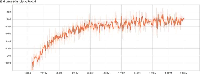
Cognitive prediction of obstacle’s movement 129
speed control behaviours and wall following, meaning the agent would navigate along the walls in the
corridor. Another example is a study focusing on the dynamic nature of the environment by Tekmono and
Millonig [14], in which the agent imitates the method humans find a path when being uncertain about
which doors are open. The agents in these models are rule-based, which means the behaviours are con-
structed using a finite set of rules. As a result, it often lacks flexibility in the choice of actions, as it could be
impossible to build these rules based on the understanding of behavioural psychology in its entirety.
The use of reinforcement learning in the agent-based model has recently become more prevalent.
Prescott and Mayhew [15] proposed a reinforcement learning method to train the agent basic collision
avoidance behaviour. Recently, Everett et al. [16] introduced a novel method for the agent to avoid colli-
sions, using reinforcement learning with deep learning. The resulted behaviours of these models are very
competent; however, the effect of human cognition is still lacking. Other studies have been trying to resolve
this problem. For instance, Chen et al. [17] proposed a deep reinforcement learning model with the agent
respecting social norms in situations such as passing, crossing and overtaking. We also proposed a rein-
forcement learning model considering the risk of the obstacle [18]; however, the model only accommodates
the pedestrian path-planning process.
Regarding research in prediction, while the studies on highly accurate prediction are extensive, espe-
cially in the robotic domain, there is not much research in the prediction by the human cognitive system.
Ikeda et al. [19] proposed an approach to the prediction of the pedestrian’s navigation employing the sub-
goal concept, meaning the navigation path would be segmented into multiple polygonal lines. We have also
addressed the concept of human prediction in our previous study [20]. However, the prediction is only
fitting for the long-term path planning of the pedestrians. In the interacting stage, on the other hand,
this often happens concurrently with the continuous actions of the agent. Within the studies in human
neuroscience, Bubic et al. [21] discussed the mechanism of the prediction in the human brain, which could
provide helpful insight into the cognitive prediction, especially in the pedestrian navigating process.
Table 1 represents a literature matrix of the works related to this study. From the literature matrix, it
could be seen that there is currently no study that utilises reinforcement learning for the interaction
behaviour of pedestrians. Risk is also a factor that is often overlooked, although it has been determined
to be a determinant factor in the pedestrian’s navigation behaviour.
3 Background
3.1 Reinforcement learning
The concept of reinforcement learning was first coined by Surton and Barto [22]. In reinforcement learning,
the agent needs to optimise the policy, which specifies the actions that will be taken under each state of the
observed environment. For each action taken, a reward signal will be given to encourage or discourage the
action. The aim of the agent is to maximise the cumulative reward in the long term. Because certain actions
could receive an intermediate negative reward but may achieve the highest conclusive reward, a value
function is necessary to estimate the present state of the agent.
The formulation for a reinforcement learning problem is often modelled as a Markov Decision Process
(MDP). An MDP is a tuple ( , , P , R, γ ) where is a finite set of states; is the set of agent’s actions; P is
the probability function which describes the state transitions from s to s′ when action a is taken, R is the
reward function immediately given to the agent; γ ∈ [0, 1] is the discount factor. To solve a reinforcement
learning problem is to find the optimal policy π : → that maximises long-term cumulative reward. The
value function for the state s would be presented as:
∞
V (s) = max E⎡ ⎤
⎢ ∑ γ R(st , π (st ))⎥ .
t (1)
⎣t=0 ⎦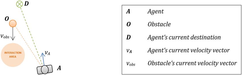
130
Table 1: Literature matrix of the related work
No Title Method Setting Findings
1 Social force model for pedestrian dynamics [6] Physics-based Basic navigation Pedestrian behaviour is driven by attraction forces to the points of interest
and repulsion forces from walls and obstacles
2 Walking ahead: The headed social force model [12] Physics-based Basic navigation The navigation of pedestrians is affected by their heading direction
3 Basics of modelling the pedestrian flow [13] Physics-based Basic navigation The relation between the pedestrian’s velocity and the required space to
navigate contributes to the Social force model
4 A behavioural dynamics approach to modelling realistic Agent-based Basic navigation Pedestrians follow the walls while navigating within the environment
pedestrian behaviour [8]
Thanh-Trung Trinh and Masaomi Kimura
5 A navigation algorithm for pedestrian simulation in Agent-based Path planning Utilising an optimisation method on a navigation matrix using maximum
dynamic environment [14] neighbourhood value to simulate the agent’s navigation towards a
possible opened door
6 Modelling and prediction of pedestrian behaviour based Agent-based Pedestrian Pedestrian agent navigates by partitioning the navigation path into
on the sub-goal concept [19] prediction multiple sections passing certain points following the sub-goal concept
7 Obstacle avoidance through reinforcement learning [15] Reinforcement learning Collision avoidance Reinforcement learning could be employed for the pedestrian agent to
perform basic obstacle avoidance actions
8 Collision avoidance in pedestrian-rich environments with Deep RL Collision avoidance Pedestrian agent learns the navigation and obstacle avoidance behaviour
deep reinforcement learning [16] using a deep reinforcement learning framework
9 Socially aware motion planning with deep reinforcement Deep RL Path planning A deep reinforcement learning model for pedestrian agents for interacting
learning [17] circumstances such as passing, overtaking, and overtaking
10 The impact of obstacle’s risk in pedestrian agent’s local Deep RL Path planning The risk from the obstacle could significantly affect the path planned by
path-planning [18] the pedestrian before navigation
11 Point-of-conflict prediction for pedestrian path- Deep RL Path planning A prediction model in the path planning process of the pedestrian agent
planning [20]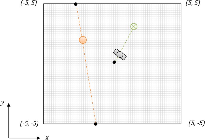
Cognitive prediction of obstacle’s movement 131
3.2 PPO algorithm
PPO algorithm, proposed by Schulman et al. [23], is a reinforcement learning algorithm using a neural
network approach to optimise the agent’s policy via a training process. The loss function of the neural
t , the deviation of the expected reward compared to the
network is constructed using an advantage value A
current state’s average reward. The clip objective of the loss function is presented as
t , clip(rt (θ ) , 1 − ε, 1 + ε )A
Lclip(θ ) = ˆ [min(rt (θ )A t )], (2)
π (a ∣ s )
where rt = π θ (ta ∣ts ) and ε is a clipping hyper-parameter. The clipping helps the training become more
θ old t t
stable, as the previous policy will not be overwritten by a worse policy in a noisy environment.
With the inclusion of policy surrogate and value function error term, the loss function in the PPO
algorithm is formulated as follows:
Lclip + VF + S (θ ) = ˆ [Lclip(θ ) − c1L VF (θ ) + c2S[πθ ](st )], (3)
where c1 and c2 are coefficients, S represents entropy bonus and L VF is the squared-error loss.
4 Methodology
The procedure of navigating in the environment of a human pedestrian could be categorised into three
levels [24]. In the first level, strategic level, the pedestrian needs to initiate the planning, such as deter-
mining the destination and planning the means to get there. The second level is the tactical level, in which
the pedestrian needs to plan the navigation path to achieve the intermediate desired goal, such as reaching
the local destination while considering possible obstructions that may hinder the navigation. For instance,
if there are obstructions like physical obstacles or other pedestrians, the agent also needs to plan forward so
that the path will not conflict with their navigation. The third level, which is the operational level, will
handle the agent’s operational dynamics such as movement or gesture controls. At this level, the agent
must act appropriately according to the short-term states of the environment.
The focus of our research in this article is the interacting process, which happens at the operational
level. An example of this interaction is when the pedestrian is getting close to another person, but that
person suddenly changes the movement in an unpredictable manner that could collide with the pedes-
trian’s planned path. In this situation, the agent needs to continuously observe the other person’s every
action, and accordingly decide which interaction or movement to make. For example, if that person moves
to the left of the pedestrian, he could go to the right or slow down to observe more responses from the other
person.
Typically, when the navigation needs to proceed to this process, the pedestrian is already close to the
obstacle, within a distance of a few metres. There is also a chance of one obstacle possibly conflicting with
the navigation of the pedestrian. The model for our setting is illustrated in Figure 1. The pedestrian agent A
has to try to get the destination D and also avoid the obstacle O (if exists). In usual circumstances, the agent
Figure 1: Pedestrian interacting environment setting.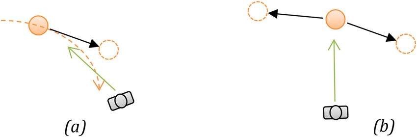
132 Thanh-Trung Trinh and Masaomi Kimura
does not always avoid the obstacle in its current position. Instead, the agent will predict the obstacle’s
navigating behaviour and avoid the future interaction area.
This learning process is similar to a child learning how to get to the destination and avoid colliding with
any obstacle. Once the behaviour is learned, he can naturally do the task simply from experience without
the need of learning again. However, as the child grows up, he would encounter many situations that he
would need to predict the movement of an obstacle to avoid stiff social behaviour. Without a proper
prediction, a pedestrian, much like the child, is likely to more frequently collide with the obstacle.
Therefore, we design our model focusing on two tasks: learning task and prediction task. The learning
task helps the agent learn the natural behaviour of navigating. The prediction task simulates the human
prediction of the obstacle’s upcoming position, which subsequently the pedestrian will avoid instead of the
obstacle’s current position.
Table 2 presents the definitions for the notations used in this article.
Table 2: Notations used in the article
Notation Definition
δA(t,)D The distance from the agent to its destination at the time t
δA(t,)O The distance from the agent to the obstacle at the time t
Ri, t The reward for the agent’s actions for the i th behaviour
κi Coefficient of the reward for the the i th behaviour
(t )
NGO The cumulative reward for the agent’s actions for all behaviours in GO category
NNB(t ) The cumulative reward for the agent’s actions for all behaviours in NB category
vt The agent’s speed at the time t
ϕt The agent’s angle at the time t
danger, size, risk The danger level, size and risk of the obstacle, respectively
τ Current time in prediction task
c Confidence rate
ε Predictability rate
4.1 Learning task
Our model uses reinforcement learning for the learning task. In reinforcement learning, the agent is
provided with different states of the environment, and it has to perform the actions corresponding to
each state. For every step, the actions which the agent carried out would affect the current states of the
environment. By specifying a reward for that result, we could instruct the agent to encourage the actions if
the reward is positive, or otherwise discourage the actions. The way the agent learns through reinforcement
learning has many similarities with the way humans learn in real life, and accordingly, it would be
beneficial to create the natural behaviour of the pedestrian agent.
To realise the reinforcement learning model for the pedestrian interaction learning task, we need to
address the following problems: designing the agent’s learning environment and proper rewarding
approach for the agent’s actions.
4.1.1 Environment modelling
Figure 2 presents the design of the learning environment for our model. Our training environment is an area
of 10 by 10 m. In each training episode, the pedestrian agent starts at (0, 0), which is the centre of the
environment. The agent will be heading to an intermediate destination, placed at a distance randomised
between 2 and 4.5 m and could be in any direction from the agent. This could be considered as a sub-goal [19]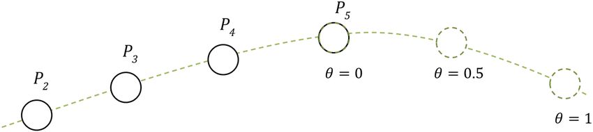
Cognitive prediction of obstacle’s movement 133
Figure 2: Learning task training environment.
of the agent for the long-term planned navigation path. For example, with the agent’s planned path to the
goal presented in our pedestrian path-planning model [18] consisting of ten component path nodes, the
intermediate destination would be the closest component node to which the agent is heading, as demon-
strated in Figure 3. The choice between planning and interacting (or the long-term task and the sub-goal task)
could be selected by using a goal-based agent system. Another approach is to realise a task allocation model
for the path-planning task and the pedestrian interacting task, similar to the method proposed by Baghaei and
Agah [25].
Figure 3: Agent’s destination as a sub-goal.
An obstacle could be randomly generated inside the environment. The obstacle is defined as another
pedestrian that could walk into the pedestrian agent’s walking area or a slow-moving physical obstacle
such as a road marking machine. We chose not to include a fast-moving object like a car in our definition of
obstacle. In that case, the entire area exclusive for its movement will be too dangerous for a pedestrian and
will be excluded from the agent’s navigation area. Regarding static obstacles, like an electric pole or a water
puddle, these could have been addressed in the planning process and could not interfere with the pedes-
trian agent’s path. From the definition, the obstacle will be randomly initialised between (−5, 5) and (5, 5) in
each training episode. After that, it will move at a fixed speed to its destination, randomly positioned134 Thanh-Trung Trinh and Masaomi Kimura
between (−5, −5) and (5, −5). With this modelling, the pedestrian agent’s path might collide with the
obstacle’s movement in any direction.
Our previous study [18] suggests that the obstacle’s danger level could moderately impact how the
agent navigates. For example, if the human pedestrian encounters a less dangerous obstacle such as
another regular pedestrian, he may alter his navigation just a bit to avoid a collision. However, if the
obstacle is a moving construction machine, the pedestrian should try to steer away from the obstacle to
avoid a possible accident.
Based on the idea of danger level, we propose a new definition called risk. Different to the obstacle’s
danger level, risk is the perception of the possibility that the danger could affect the agent. For instance, if
the agent feels an object could be dangerous, the risk would be appropriately high. However, if the chance
of the danger affecting the agent is low, the risk is accordingly reduced. Both danger level and risk in our
research represent the concepts in the agent’s cognitive system and do not reflect the actual danger of the
obstacle.
Another important factor is the size, which is the affected area of the obstacle. For instance, if the
obstacle is a group of multiple pedestrians walking together instead of one, the whole group should be
treated as a single large-sized obstacle, as suggested by Yamaguchi et al. [26]. In our model, the size of the
obstacle is randomised between 0.5 and 2; the danger level is randomised between 0 and 1 at the beginning
of each training episode. When the prediction of the obstacle’s movement is used, the risk of the obstacle
will be used instead of its danger level. The formulation of risk is presented in Section 4.2.3.
4.1.2 Agent’s observations and actions
In each step, the agent will observe various states of the environment before taking action. We have
considered two possible approaches to the design of the agent’s observations and actions. The first
approach is using Euclidean coordinates. This means the relative position of the obstacle and the destina-
tion as well as the obstacle’s direction in Euclidean coordinates will be observed. For example, assuming
the current agent’s position and obstacle’s position are (xa, ya) and (xo, yo), respectively, the agent needs to
observe the related position of the obstacle, in this case, that would be the two values (xo − xa) and ( yo − ya).
Since a neural network is used for training, this could lead to a problem of finding a relationship between
the coordinates and the rewarding. For instance, when the agent moves, the x (or y) coordinate may
increase or decrease. However, the increment or decrement of the value does not have a direct correlation
with the increment or decrement of the cumulative reward. Increasing the number of network’s hidden
layers could be more effective, but even then it would be more complicated for the neural network to find an
optimal policy.
The second approach, which is using radial coordinate, could resolve this problem. Instead of using the
coordinates in x and y values, the agent’s observations and actions would instead use the distance and
angle (relative to the local position and heading of the agent). This is helpful for the neural network to
specify the relationship between the input and the output. For instance, a low angle and a short distance to
the obstacle means that the obstacle is close; therefore, going straight (angle close to 0) could lead to a
lower reward value.
The typical downside of using radial coordinate is angle calculation, e.g. calculation of the change in
distance and angle if both the agent and the obstacle are moving. However, in the interacting process, the
interval between two consecutive steps is very small; therefore, the changes in the distance and angle are
minimal. For this reason, we adopt the radial coordinate approach for the observations and actions of the
agent.
More specifically, the observations of the environment’s states consist of: (1) the distance to the current
destination; (2) the body relative direction to the destination (from agent’s forward direction); (3) the
presence of the obstacle. The obstacle is considered present only if it is within the agent’s field of vision.
If the obstacle is observable by the agent, the agent will also observe: (4) the distance to the obstacle; (5) theCognitive prediction of obstacle’s movement 135
body relative direction to the obstacle; (6) the obstacle’s body relative direction to the agent (from the
obstacle’s forward direction); and (7) the obstacle’s speed, size and danger level.
The possible actions which the agent could perform consist of: (1) the desired speed and (2) the angle
change in the direction from the current forwarding direction. The above step will be repeated until the
agent reaches the destination, the agent gets too far from the destination or it takes too long for the agent to
reach the destination. After that, the total reward will be calculated to let the agent know how well it has
performed the task. The details of the rewarding will be explained in the next section. Finally, the environ-
ment will be reinitialised, and the agent will repeat the above steps. The set of agent’s observations and
actions, as well as the cumulative reward, is sent to be trained in a neural network aiming at maximising the
cumulative reward value.
4.1.3 Rewarding behaviour
We design the rewarding behaviour for our model based on the idea of human comfort, as suggested from
our previous study [27] in the path-planning process, which also utilised reinforcement learning. The idea
was brought by Kruse et al. [1], proposing a concept of how different factors in robot movements make
humans feel natural or comfortable. This concept is effective in our rewarding mechanism thanks to its
correlation with the method humans learn in real life. For instance, in pedestrian movement in real-life,
certain manners could be considered “natural,” like walking at a consistent speed or moving in a straight
direction to the flow of the navigation. Such manners need to be learned gradually from when a person is a
child until he is grown up. By providing the appropriate rewarding, our model’s pedestrian agent would be
able to learn a human-like walking behaviour.
There are numerous factors in the concepts of human comfort. The ones used in our model, which are
relevant to the pedestrian interacting process, are listed below. These factors are grouped into two cate-
gories: Goal Optimisation (GO) and Natural Behaviour (NB).
The category GO consists of the behaviours which encourage the agent to achieve the goal in the most
efficient way. The following factors are put under this category.
4.1.3.1 Reaching destination reward
The agent receives a small penalty every step. This is to encourage the agent to achieve the goal as swiftly as
possible. The agent also receives a one-time reward when reaching the destination. This also leads to the
termination of the current episode and resets the environment. The formula for this reward at time t is
calculated by:
(t )
⎧ Rstep , if δA, D ≥ δmin,
R1, t = (4)
⎨ Rgoal , if δA(t,)D < δmin,
⎩
where δA(t,)D is the distance between the agent and its destination at the time t ; Rstep is a small constant
penalty value for every step that the agent makes; Rgoal is the constant reward value for reaching the
destination.
4.1.3.2 Matching the intended speed
The agent is rewarded for walking at a desired speed. This value varies between people. For example, a
healthy person often walks at a faster speed than the others, while an older person usually moving at a
slower speed.
The reward for this is formulated as follows:136 Thanh-Trung Trinh and Masaomi Kimura
R2, t = −∥vt − vdefault∥, (5)
where vt is the current speed and vdefault is the intended speed of the agent.
4.1.3.3 Avoid significant change of direction
Constantly changing direction could be considered unnatural in human navigation. Appropriately, the
agent is penalised if the change in direction of the agent is greater than 90 ∘ in 1 s. The reward for this
behaviour is formulated as follows:
ϕΔ
R3, t = −Rangle , if > 90, (6)
Δt
where ϕΔ is the change in agent’s direction, having the same value as action (2) of the agent; Δt is the delta
time, the time duration of each step; and Rangle is the constant penalty value for direction changes.
The category NB consists of the behaviours which encourage the agent to behave naturally around
humans. As the navigation model in our research is fairly limited, such interactions as gestures or eye
movement cannot be implemented. Consequently, for this category, we currently have one factor.
4.1.3.4 Trying not to get too close to another pedestrian
The reward for this behaviour is formulated as follows:
⎧− danger, if size δA(t,)O < 1,
⎪ (t )
⎪⎛ δA, O − 1 ⎞
R4, t = ⎜ − 1⎟danger, if 1 ≤ size δA(t,)O < S , (7)
⎨ S−1
⎪⎝ ⎠
⎪ 0, if size δA(t,)O ≥ S ,
⎩
where δA(t,)O is the distance between the agent and the obstacle at time t ; danger and size are the danger level and
the size of the obstacle, respectively; S is the distance to the obstacle which the agent needs to start interacting
with. As mentioned in Section 4.1.1, danger is the agent’s perception of the obstacle’s danger. This will be updated
with risk when a prediction of obstacle’ movement is formed, which will be presented in Section 4.2.3.
In normal circumstances, for example, when a pedestrian is walking alone or when he is far away from
other people, the pedestrian does not have to worry about how to interact naturally with others. As a result,
the behaviours listed in the NB category need less attention than other behaviours listed in the GO category.
On the contrary, when the pedestrian is getting close to the other, the GO behaviours should be considered
less important. As a result, the cumulative reward for each training episode is formulated as follows:
n
= (t )
∑h(NGO (t )
, NNB ), (8)
t=1
where h is a heuristic function to combine the rewards for achieving the goal and the rewards for providing
(t )
the appropriate human behaviour; n is the number of steps in that episode; NGO is the sum of the cumulative
(t )
rewards for all behaviours in GO category at time t and NNB is the sum of the cumulative rewards for all
behaviours in NB category at time t .
(t )
NGO = κ1R1, t + κ2R2, t + κ3R3, t , (9)
(t )
NNB = κ4R4, t , (10)
where κ1 is the coefficient for reaching destination rewarding; κ2 is the coefficient for matching intended
speed rewarding; κ3 is the coefficient for changing direction avoidance rewarding; κ4 is the coefficient for
collision avoidance rewarding.Cognitive prediction of obstacle’s movement 137
Different people have different priorities for each previously mentioned behaviour. As a result, with
different coefficient values of κ1 , κ2 , κ3 and κ4 , an unique pedestrian personality could be formulated.
The heuristic function is implemented in our model as follows:
n
= (t )
∑(γNGO (t )
+ (1 − γ )NNB ), (11)
t=1
where γ is a value ranging from 0 to 1, corresponding to how far the agent is from the obstacle and also the
size of the obstacle. The reason for including the size of the obstacle in the calculation of γ is that when an
obstacle is bigger, it would appear closer to the pedestrian, and the pedestrian may want to be further away
from the obstacle as a result. Therefore, γ is specified in our model as follows:
1
γ= , (12)
δA, Osize + 1
where δA, O is the distance between the agent and the obstacle; size is the observed size of the obstacle.
4.2 Prediction task
The predictive process happens in almost every part of the brain. This is also the cause of many bias signals
sent to the cognitive process, leading to the behaviour in which humans act in real life [21]. In the human
brain, the prediction is made using information from past temporal points, then it would be forwarded to be
compared with actual feedback from sensory systems. The accuracy of the prediction is then used to update
the predictive process itself.
The prediction task helps the agent avoid colliding with the obstacle more efficiently. Without using a
prediction, the pedestrian might interrupt the navigation of the other pedestrian or even collide with. This
behaviour is more frequently observable in younger pedestrians, whose prediction capability has not been
fully developed.
The prediction task could happen in both the path-planning process and the interacting process. For
example, when a person observes another pedestrian walking from afar, he could form a path to avoid the
collision. In our previous research, we proposed a prediction model for the path-planning process by
combining both basic direction forwarding and using a path-planning reinforcement learning model to
estimate the possible point-of-conflict [20]. The evaluation result shows that the pedestrian agent could plan
a more efficient and realistic navigation path.
The prediction in the interacting process is, however, different from the prediction in the path-planning
process. While in the path-planning process, the agent only needs to project an approximate position of the
obstacle in order to form a path, in the interacting process the agent will need to carefully observe every
movement of the obstacle to expect its next actions. This will be carried out continuously when the agent is
having the obstacle in sight.
For this reason, a simple position forwarding prediction could not be sufficient. The first problem with
this is that when the obstacle is moving with a certain pattern (e.g., the obstacle is moving along a curve, as
shown in Figure 4a), a position forwarding prediction using only the obstacle’s direction is usually
Figure 4: The problems with the position forwarding prediction model. (a) Obstacle moves along a curve; (b) Obstacle is
uncertain about its orientation.138 Thanh-Trung Trinh and Masaomi Kimura
incorrect. The second problem is that when the obstacle is uncertain about its orientation and choosing to
move in two opposite directions. The agent may see the position in the centre is safe to navigate (as shown
in Figure 4b), while actually, it is usually the contrary.
In order to solve these problems, we had to look into the mechanism of the predictive process. Based on
that, we set up three steps for the prediction task, presented as follows:
Step 1 – Estimation: Based on the previous movement of the obstacle, the pedestrian agent forms a
trajectory of its movement. Subsequently, the agent specifies the location in that trajectory that he thinks
the obstacle would be at the current moment.
Step 2 – Assessment: The difference between the predicted location and the actual current position of
the obstacle is measured. This indicates how correct the prediction was, meaning how predictable the
movement of the obstacle was. If the predicted location is close to the actual position, it means the move-
ment of the obstacle is fairly predictable, thus the agent could be more confident in predicting the future
position of the obstacle.
Step 3 – Prediction: The agent forms a trajectory of the obstacle’s movement based on the current
movement. Combining with the difference calculated in Step 2, the agent predicts the future position of the
obstacle on that trajectory. If the difference is small, meaning that the agent is confident with the prediction,
he would predict a position further in the future and vice versa.
Figure 5: Prediction task model.
Figure 5 illustrates the modelling of the prediction task. P1, P2 , P3, P4 and P5 are the sampled positions of
the obstacle’s movement, with P5 is the obstacle’s current position. Pe is the projected position of the
obstacle from P1 to P4 and Ppredict is the predicted position of the obstacle. The flowchart for the prediction
process is presented in Figure 6.
As an example, if a pedestrian obstacle is going straight in one direction, its movement could be easily
figured. Consequently, the difference between its predicted location and its actual current position should
be fairly small. The agent then will be able to predict the obstacle’s position further in the future and will be
able to comfortably avoid it. On the other hand, if the pedestrian is moving unpredictably, it will be very
difficult for the agent to guess its movement. In this case, the predicted location of the obstacle in the future
would be mostly incorrect. Consequently, avoiding the near future or even the current projection of the
obstacle would be a better decision.Cognitive prediction of obstacle’s movement 139
Figure 6: Prediction process flowchart.
4.2.1 Estimation
The recent position data of the obstacle are stored together with its respective time information in a data
structure by logging the data every fixed timeframe. To avoid the incorrect data being logged, the timeframe
should be longer than the time duration between two continuous frames.
First of all, the agent needs to form a trajectory of the obstacle’s movement from the past positions. To
do that, the agent will need to choose some samples from previously recorded location data of the obstacle,
then perform interpolation to get a parametric representation of the movement.
To help the agent with choosing the sample and performing interpolation, we propose a concept called
confidence rate. The confidence rate of the agent, denoted by c , is a value which is dependent on the
accuracy of the agent’s previous prediction. With a high confidence rate, the agent could be more comfort-
able interpolating using a wider time span. The confidence rate will be calculated in the assessment step,
presented in Section 4.2.2.
For the interpolation process, we used two Lagrange polynomial interpolations. One interpolation is
used for the set of (xi , ti ) and the other is used for the set of ( yi , ti ). For the interpolating polynomial
presented in the form of a cubic function, four sets of samples corresponding to t1 … t4 are required.
Given the current time τ , the value ti is calculated as follows:
ti = τ − (5 − i )Δ, (13)
with
Δ = cγ1, (14)
where c is the confidence rate ranging from 0 to 1; γ1 is a time constant discount. For example, if the agent is
very confident (c = 1) and the samples chosen from the pedestrian obstacle’s previous movement of 2 s,
then γ1 could be 0.4.
We set a minimum value of 0.3 for Δ as in reality, human perception cannot recognise the object’s
micro-movement. Therefore, in the case of a low confidence rate (e.g., when the previous prediction140 Thanh-Trung Trinh and Masaomi Kimura
was greatly incorrect), the pedestrian agent will still use samples from the obstacle’s previous 1.5 s
approximately.
The four sets of the corresponding (xi , ti ) and ( yi , ti ) are used to specify the x = x (t ) and y = y (t )
functions using Lagrange interpolation. Specifically, the x = x (t ) function is formulated from (x1, t1)…(x4, t4)
as follows:
(t − t2 )(t − t3)(t − t4) (t − t1)(t − t3)(t − t4)
x= x1 + x2
(t1 − t2 )(t1 − t3)(t1 − t4) (t2 − t1)(t2 − t3)(t2 − t4)
(15)
(t − t1)(t − t2 )(t − t4) (t − t1)(t − t2 )(t − t3)
+ x3 + x4 .
(t3 − t1)(t3 − t2 )(t3 − t4) (t4 − t1)(t4 − t2 )(t4 − t3)
The y = y (t ) function is similarly specified.
The estimation of the current position of the obstacle Pe(xe , ye ) at the current time τ is defined
by: (xe , ye ) = (x (τ ) , y (τ )).
4.2.2 Assessment
The predictability of the obstacle’s movement is calculated using the distance δe between the obstacle’s
current position (x5, y5) and the estimated position of the agent (xe , ye ) as calculated above. If δe is small, it
means the movement is predictable. On the contrary, if δe is large, it means the movement is not as the agent
expected. An example of this is when a pedestrian encounters an obstacle, which is another pedestrian
walking in the opposite direction. When trying to avoid running into the obstacle, the pedestrian observes
that the movement of the obstacle was going to his left-hand side. However, the obstacle makes a sudden
change and walk to the right instead. This makes the movement of the obstacle seemingly unpredictable,
and thus the pedestrian needs to be more careful when planning to interact.
We defined a value predictability rate as ε , determined by:
1
ε= ,
5 (16)
( δe
D
+1 )
where D is the average distance between the first and the last sample points P1 and P4 .
The confidence rate c will then be calculated using the predictability rate. The confidence rate gets
higher or the agent is more confident when ε is consecutively at a high value and vice versa. The formula-
tion for calculating the confidence rate could be different for each person, as some people could be more
confident after several correct predictions than others.
The formulation for calculating the confidence rate ct at time t is presented as follows:
ct = ct − 1 + γ2 (εt − ct − 1) , (17)
where γ2 is the discount for the change in confidence rate, with γ2 = 0 meaning the confidence rate is not
dependent on the prediction rate, and γ2 = 1 meaning the confidence rate will always equal the prediction
rate. Practically, γ2 should be from 0.3 to 0.6.
4.2.3 Prediction
Similar to the estimation step, we also use Lagrange interpolation in the Prediction to form the functions
x = x¯ (t ) and y = y¯ (t ) for the projection of the movement. In this step, however, the sample positions used
are P2 to P5 (the current position of the obstacle), respectively. Specifically, the function x = x¯ (t ) for the four
sets of samples (x2 , t2 )…(x5, t5) is presented as:Cognitive prediction of obstacle’s movement 141
(t − t3)(t − t4)(t − t5) (t − t2 )(t − t4)(t − t5)
x= x2 + x3
(t2 − t3)(t2 − t4)(t2 − t5) (t3 − t2 )(t3 − t4)(t3 − t5)
(18)
(t − t2 )(t − t3)(t − t5) (t − t2 )(t − t3)(t − t4)
+ x4 + x5.
(t4 − t2 )(t4 − t3)(t4 − t5) (t5 − t2 )(t5 − t3)(t5 − t4)
The y = y¯ (t ) function is similarly specified.
The prediction of the obstacle is determined from the functions x = x¯ (t ) and y = y¯ (t ) at the time
ti = τ + θ , where τ is the current time and θ is the forward time duration in the future. Consequently, if
the agent wants to predict the location of the obstacle at 1 s in the future, θ would be 1. Figure 7 demon-
strates how different θ value affects the resulted prediction of the obstacle.
Figure 7: Resulted predictions with different θ .
θ depends on the confidence rate c . If the agent is confident with the prediction, he will predict an
instance of the obstacle at a further point in the future. On the contrary, if the agent is not confident, for
example when the obstacle is moving unpredictably, he would only choose to interact with the current state
of the obstacle (θ close to 0). The estimation of θ in our model is formulated as follows:
θ = cεγ3, (19)
where γ3 is a time constant discount. For example, when the agent is confident, the current prediction is
correct and the forward position of the obstacle could be chosen at 1 s in the future, γ3 could be set to 1.
To summarise, the function to calculate the predicted position (xp, yp) of the obstacle could be for-
mulated as follows:
(xp, yp) = (x¯ (τ + cεγ3) , y¯ (τ + cεγ3)) . (20)
Finally, the predicted position of the obstacle will be assigned to the observation of the agent as
presented in Section 4.1. More specifically, instead of observing the current position of the obstacle, the
agent will use the predicted position (xp, yp) of the obstacle.
The risk of the obstacle, as mentioned in Section 4.1.1, will be updated depending on the confidence
rate of the agent. One reason for this is when an obstacle is moving unpredictably, it could be hard to expect
where it could go next, which leads to a higher risk assessed by the agent. The relation between the
obstacle’s risk and danger level is defined as follows:
r = danger + (1 − danger)(1 − c ) , (21)
where r is the risk, danger is the danger level of the obstacle perceived by the agent and c is the confidence
rate of the agent. That means if the agent is confident with the movement of the obstacle, the perceived risk
will be close to the danger level observed by the agent. However, if the confidence rate is low, the risk will
be increased correspondingly.
5 Implementation and discussion
Our proposed model was implemented with C# using Unity 3D. We prepared two separate environments for
the implementation. One environment is used for the agent training of the learning task and the other for142 Thanh-Trung Trinh and Masaomi Kimura
implementing the prediction task as well as to validate our model. The source code for our implementation
could be found at https://github.com/trinhthanhtrung/unity-pedestrian-rl. The two environments are
placed inside the Scenes folder by the names InteractTaskTraining and InteractTaskValidate, respectively.
Figure 8 presents our implementation application running in the Unity environment.
Figure 8: A screenshot from the implementation application.
For the training of the learning task, we used the Unity-ML library by Juliani et al. [28]. The environ-
ment’s states together with the agent’s observations and actions are constructed within Unity. The signals
are then transmitted via Unity-ML communicator to their Python library to be trained using a neural
network. Afterwards, the updated policy will be transferred back to the Unity environment. For our
designed training environment, the pedestrian agent has the cumulative reward converged after 2 million
steps, using a learning rate of 3 × 10⁻⁴ . The computer we used for the training is a desktop computer equipped
with a Core i7-8700K CPU, 16 GB of RAM and NVIDIA GeForce GTX1070 Ti GPU. With this configuration, it took
1 h 40 min to complete the process. The statistics for the training is shown in Figure 9.
Figure 9: Learning task training statistics.
For the predicting task, we created a script called movement predictor and assigned it to the pedestrian
agent. The position records of the obstacle are stored in a ring buffer. The advantage of using a ring buffer is
the convenience of accessing its data: with the confidence rate specified, the time complexity to get the dataCognitive prediction of obstacle’s movement 143
of the obstacle’s past locations is always O(1). The values γ1, γ2 and γ3 in (14), (17), (19) are set to 1.7, 0.45,
and 1.1, respectively.
The demonstration of our pedestrian interacting behaviour could be observed from the following
page: https://github.com/trinhthanhtrung/unity-pedestrian-rl/wiki/Demo. The user could freely control
an obstacle and interact with the agent. In our experiment, we controlled the obstacle to walk and interact
with the agent in similar behaviour as an actual person using existing pedestrian video datasets. From the
demonstration, it could be seen that the movement of the pedestrian agent bears many resemblances with
the navigation of actual humans. The pedestrian agent is able to successfully avoid the obstacle most of the
time and reach the destination within a reasonable amount of time. This result suggests that basic naviga-
tion behaviour could be achieved by the agent by utilising reinforcement learning, thus confirming this
study’s hypothesis as well as the suggestion by other researchers [29]. By incorporating the prediction
process, the agent also expressed avoidance behaviour by moving around the back of the obstacle instead
of passing at the front, similar to how a human pedestrian moves. In case of an obstacle with unpredictable
behaviour, the agent shows certain hesitation and navigates more carefully. This also coincides with
human movement behaviour when encountering a similar situation, consequently introducing a more
natural feeling when perceiving the navigation, corresponding to our expectations.
On the other hand, several behavioural traits of human navigation were not presented in the navigation of
our model’s implementation. An example is that a human pedestrian in real life may stop completely when
the collision is about to happen. This is for the pedestrian to carefully observe the situation and also to make it
easier for the other person to respond. In our model, the agent only slightly reduces its velocity. Another
example is when interacting with a low-risk obstacle, the agent may occasionally collide with the obstacle.
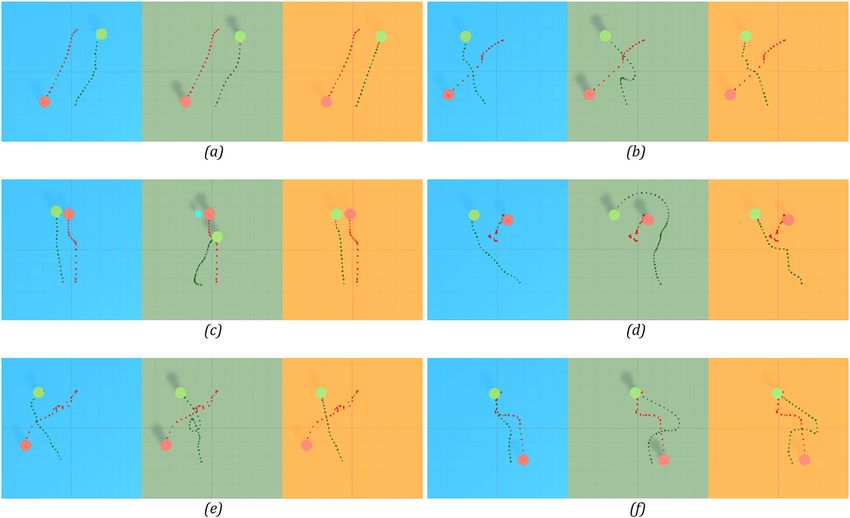
To evaluate our model, we compared our results with a Social Force Model (SFM) implementation and
the built-in NavMesh navigation of Unity. Some examples of the implementation are demonstrated in
Figure 10. In each situation, our cognitive reinforcement learning model is on the left (blue background),
the Social force model implementation is in the middle (green background), and the Unity NavMesh
implementation is on the right (yellow background). The green circle represents the agent and the red
Figure 10: Example interacting situations between agent and obstacle in comparison with Social Force Model and Unity
NavMesh. The green circle represents the agent and the red circle represents the obstacle. (a) The agent and the obstacle move
in two opposite directions; (b) The obstacle crosses path with the agent; (c) The obstacle obstructs the agent's path to the
destination; (d) The obstacle moves slowly around the agent; (e) The obstacle moves slowly intersecting the agent's path; (f)
The obstacle unexpectedly changes its direction.144 Thanh-Trung Trinh and Masaomi Kimura
circle represents the obstacle. The green and the red spots are the periodically recorded positions of the
agent and the obstacle, respectively.
Upon observation of each model’s behaviour, the difference in the characteristics of its movement could
be noticed. As the SFM model is realised using a force-based method, the movement of the pedestrian agent
in SFM is very similar to a magnetic object. The appearance of an obstacle could push away the agent when
it is being close. The agent in the Unity NavMesh implementation often takes the shortest path approach.
However, as the agent only considers the current state of the environment, it may occasionally take a longer
path when the obstacle moves. On the other hand, the behaviour of the agent in our model is more
unpredictable, although certain factors such as taking the shorter path and collision avoidance are still
considered. Except for the NavMesh implementation, both implementations of our model and SFM could
demonstrate the behaviour of changing the agent’s speed. While the agent in SFM often changes the speed
to match the obstacle’s velocity, the agent in our model tends to slow down when being close to the
obstacle.
In the most basic situations, when there are two pedestrians walking in opposite directions as simu-
lated in (a), all models could demonstrate acceptable navigating behaviour. These are also the most
common situations observed in real life. However, the difference between the implementations is most
evident when in certain scenarios in which the obstacle does not follow the usual flow of the path, such as
in other situations presented in Figure 10. These are modelled from the real-life pedestrians in the cases
when, for instance, a person crossed the path, a person was walking while looking at his phone without
paying much attention to the others or a person suddenly noticed something and changed his path towards
that place. While our implementation shows natural navigation in all test scenarios, the SFM and NavMesh
implementations show many unnatural behaviours. This could be seen in situation (f) for NavMesh imple-
mentation, where the agent takes a wide detour to get to the destination. For SFM implementation, the
agent demonstrates much more inept behaviour, notably seen in situations (b), (d), (e), and (f). Another
problem of the SFM’s implementation could be seen in (c). In this circumstance, the pedestrian agent is
unable to reach its destination, as the force from the obstacle keeps pushing the agent away. On the
contrary, the problem with NavMesh’s agent is that the agent continuously collides with the obstacle.
This is most evident in the situation (d) and (e), in which the agent got very close to the obstacle, then
walked around the obstacle, greatly hindering the obstacle’s movement. Arguably, this behaviour could be
seen in certain people; however, it is still considered impolite or ill-mannered. The agent in our imple-
mentation suffers less unnatural behaviour compared to the others. Take the situation (f) for example, while
the obstacle was hesitant, the agent could change the direction according to how the obstacle moves.
We also compared our implementation with SFM and NavMesh using the following aspects: the path
length to reach the destination, the navigation time and the collision time (i.e. the time duration that the
agent is particularly close to the obstacle). These are some common evaluation criteria, which are used in
many studies to evaluate the human likeness of the navigation. To evaluate these aspects, we ran a total of
121 episodes of the situations modelled from similar settings from real life. Each episode starts from when
the agent starts navigating to when the destination is reached, or when the end time limit of the simulated
situation has been reached. The collision time is specified by measuring the time that the distance between
the agent and the obstacle is less than the sum of the radius values of the agent and the obstacle. The
average results are shown in Table 3. Compared to our model, the Social force model agent took a con-
siderably longer path as the agent always wanted to keep a long distance from the obstacle. Consequently,
the average time to complete the episode of the Social force model agent is much higher than ours.
Table 3: Comparisons with social force model and unity NavMesh in average length, time and collisions
Cognitive RL Social force model Unity NavMesh
Average path length (m) 5.134 5.608 4.987
Average navigation time (s) 4.142 4.965 3.881
Average collision time (s) 1.182 0.291 1.267You can also read