Characterizing coastal phytoplankton seasonal succession patterns on the West Antarctic Peninsula
←
→
Page content transcription
If your browser does not render page correctly, please read the page content below
19395590, 0, Downloaded from https://aslopubs.onlinelibrary.wiley.com/doi/10.1002/lno.12314, Wiley Online Library on [05/02/2023]. See the Terms and Conditions (https://onlinelibrary.wiley.com/terms-and-conditions) on Wiley Online Library for rules of use; OA articles are governed by the applicable Creative Commons License
                                                                                                                                       Limnol. Oceanogr. 9999, 2023, 1–17
                                                                                    © 2023 The Authors. Limnology and Oceanography published by Wiley Periodicals LLC on
                                                                                                  behalf of Association for the Sciences of Limnology and Oceanography.
                                                                                                                                                  doi: 10.1002/lno.12314

Characterizing coastal phytoplankton seasonal succession patterns
on the West Antarctic Peninsula
Schuyler C. Nardelli ,1* Patrick C. Gray ,2 Sharon E. Stammerjohn ,3 Oscar Schofield                                                         1
1
 Rutgers University Center for Ocean Observing Leadership, Rutgers University, New Brunswick, New Jersey
2
 Duke University Marine Lab, Duke University, Beaufort, North Carolina
3
 Institute of Arctic and Alpine Research, University of Colorado, Boulder, Colorado

          Abstract
             In coastal West Antarctic Peninsula (WAP) waters, large phytoplankton blooms in late austral spring fuel a
          highly productive marine ecosystem. However, WAP atmospheric and oceanic temperatures are rising, winter
          sea ice extent and duration are decreasing, and summer phytoplankton biomass in the northern WAP has
          decreased and shifted toward smaller cells. To better understand these relationships, an Imaging FlowCytobot
          was used to characterize seasonal (spring to autumn) phytoplankton community composition and cell size dur-
          ing a low (2017–2018) and high (2018–2019) chlorophyll a year in relation to physical drivers (e.g., sea ice and
          meteoric water) at Palmer Station, Antarctica. A shorter sea ice season with early rapid retreat resulted in low
          phytoplankton biomass with a low proportion of diatoms (2017–2018), while a longer sea ice season with late
          protracted retreat resulted in the opposite (2018–2019). Despite these differences, phytoplankton seasonal suc-
          cession was similar in both years: (1) a large-celled centric diatom bloom during spring sea ice retreat; (2) a peak
          summer phase comprised of mixotrophic cryptophytes with increases in light and postbloom organic matter;
          and (3) a late summer phase comprised of small (< 20 μm) diatoms and mixed flagellates with increases in wind-
          driven nutrient resuspension. In addition, cell diameter decreased from November to April with increases in
          meteoric water in both years. The tight coupling between sea ice, meltwater, and phytoplankton species
          composition suggests that continued warming in the WAP will affect phytoplankton seasonal dynamics, and
          subsequently seasonal food web dynamics.

   Coastal waters along the West Antarctic Peninsula (WAP)                      Phytoplankton blooms along the WAP initiate in the austral
host a highly productive, ice-dependent marine ecosystem                        spring when increased solar irradiance alleviates light limitation,
fueled by large, seasonal phytoplankton blooms reaching                         and sea ice melt stratifies the upper water column and confines
chlorophyll a (Chl a) concentrations > 20 mg m3 (Vernet                        phytoplankton in well-lit surface waters (Vernet et al. 2008;
et al. 2008; Ducklow et al. 2013; Kim et al. 2018). Average pri-                Venables et al. 2013). Macronutrients and micronutrients are
mary productivity in the WAP is  182 g C m2 yr1, which is                    generally replete in coastal WAP waters (Kim et al. 2016; Sherrell
similar to other continental shelf areas in Antarctica (Arrigo                  et al. 2018; Carvalho et al. 2020), thus upper water column
et al. 2008), but four times lower than other productive coastal                stratification is considered the primary driver of phytoplankton
regions in the world’s oceans (Vernet and Smith 2007).                          productivity (Garibotti et al. 2005a; Vernet et al. 2008; Car-
                                                                                valho et al. 2020). Interannual phytoplankton dynamics are
                                                                                tightly coupled to krill recruitment (Saba et al. 2014), and
*Correspondence: scn50@scarletmail.rutgers.edu
                                                                                krill in turn are the main food source for penguins, seals,
This is an open access article under the terms of the Creative Commons          whales, and other predators (Ducklow et al. 2013),
Attribution-NonCommercial License, which permits use, distribution and          suggesting a strong bottom-up control of the ecosystem.
reproduction in any medium, provided the original work is properly cited
and is not used for commercial purposes.
                                                                                Thus, studying how coastal phytoplankton communities
                                                                                respond to physical drivers is imperative for understanding
Additional Supporting Information may be found in the online version of         ecosystem structure and function.
this article.
                                                                                   The coastal WAP phytoplankton community is comprised
Author Contribution Statement: S.N. and O.S. designed the study                 of diatoms, cryptophytes, mixed flagellates, prasinophytes,
and analysis. S.N. and S.S. acquired data. S.N., S.S., and P.G. performed       and haptophytes, with diatoms making up the highest per-
data analysis. S.N. prepared figures and drafted the original manuscript.
S.N., P.G., S.S., and O.S. helped with interpretation of data and edited        centage of annual biomass (Varela et al. 2002; Garibotti
the manuscript.                                                                 et al. 2005a; Schofield et al. 2017). However, different

                                                                            1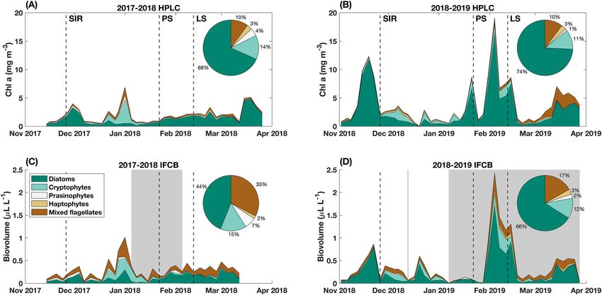
19395590, 0, Downloaded from https://aslopubs.onlinelibrary.wiley.com/doi/10.1002/lno.12314, Wiley Online Library on [05/02/2023]. See the Terms and Conditions (https://onlinelibrary.wiley.com/terms-and-conditions) on Wiley Online Library for rules of use; OA articles are governed by the applicable Creative Commons License
Nardelli et al.                                                                           WAP coastal phytoplankton seasonal succession

phytoplankton species require specific abiotic conditions for            This technique uses marker pigments of phytoplankton groups
optimal growth, causing both seasonal and interannual vari-             to assess their contributions to overall abundance. Few studies
ability in community composition. Earlier studies have tried            have looked at higher taxonomic resolution and cell size
to reconstruct seasonal succession at Palmer Station; however,          distributions over seasonal scales along the WAP.
validation of these hypotheses is still an open question as the            Our study utilized an imaging-in-flow cytometer to character-
results are either based on phytoplankton accessory pigments            ize seasonal and interannual phytoplankton diversity at Palmer
only capable of resolving general taxa (Schofield et al. 2017),          Station, Antarctica, with a focus on local sea ice and meltwater
or do not span a full austral spring to autumn range (Garibotti         impacts. We sampled both a high and low Chl a year to investi-
et al. 2005a). In general, these studies found three successional       gate (1) interannual differences in the physical environment
phases in the coastal WAP: (1) a diatom-dominated bloom                 and corresponding differences in phytoplankton communities,
comprised primarily of large centric diatoms associated with            and (2) potential mechanisms driving phytoplankton seasonal
spring sea ice retreat and upper water column stratification in          succession. Results showed that despite significant differences in
November/December, (2) a cryptophyte-dominated commu-                   sea ice dynamics and phytoplankton biomass between years,
nity associated with low Chl a, decreased nutrient stocks, and          there were consistent seasonal succession patterns. In addition,
shallow mixed layer depths in December/January, and (3) a               environmental disturbances (e.g., spring sea ice retreat, upper
diatom-enriched assemblage associated with low Chl                      water column mixing, glacial melt, and sea ice melt) throughout
a including small diatoms, haptophytes, and unidentified fla-             the growing season drove changes in phytoplankton commu-
gellates in February/March.                                             nity composition that could not be described using HPLC alone.
   Significant environmental change is impacting the produc-             These findings provide insights into regulation of WAP seasonal
tive WAP ecosystem. One of the fastest warming regions on               phytoplankton dynamics and help hypothesize how ongoing
Earth, WAP winter air temperatures and surface ocean temper-            warming and melting might impact future coastal phytoplank-
atures have increased by > 6 C and > 1 C, respectively, since         ton communities.
1951 (Meredith and King 2005; Turner et al. 2005). In
response, 90% of marine glaciers were in retreat as of 2016,
                                                                        Methods
the annual sea ice season has decreased by > 92 d since 1979,
and there is no longer perennial sea ice in the northern WAP            Sample collection
(Stammerjohn et al. 2012; Cook et al. 2016). Ocean warming,                Annual sample collection at Palmer Station, Antarctica
sea ice and glacial retreat, and glacial melt have in turn              (Fig. 1) has been conducted by the PAL-LTER since 1991 at
impacted the phytoplankton community, with significant                   two locations: an inshore station (Sta. B, bottom depth of
decreases in January mean phytoplankton biomass along the                75 m) and an offshore station (Sta. E, bottom depth of
northern WAP corresponding with a shift from large                       200 m). These stations are sampled twice per week from
(> 20 μm) to small-celled (< 20 μm) phytoplankton (Montes-              approximately early November (when the sea ice cover breaks
Hugo et al. 2009). It is hypothesized that this size shift is           up) to late March. Inclement weather and heavy sea ice can
driven by increasing cryptophyte (cell diameters of  6.5–              impede sampling in this region, leading to occasional gaps in
9 μm) abundance in coastal regions that are often associated            the dataset. Our study focused on two austral summer field
with low salinity meltwater (Moline et al. 2004; Mendes                 seasons: 2017–2018 (16 November–26 March), which had
et al. 2013; Schofield et al. 2017). The reasons why                     lower than average Chl a and was preceded by a shorter than
cryptophytes might outcompete diatoms in low-salinity                   average winter sea ice duration, and 2018–2019
waters are not well understood, but are hypothesized to be              (02 November–28 March), which had higher than average Chl
related to an advanced light-adaptation system that allows              a and was preceded by a longer than average winter sea ice
them to thrive in stratified surface waters with high irradi-            duration (Fig. S1). Because we were interested in the impacts
ances (Kaňa et al. 2012; Mendes et al. 2018a). The increased           of sea ice and glacial meltwater on inshore phytoplankton
spatial extent of low salinity surface waters is predicted to           communities, our analysis exclusively used surface samples
increase the prevalence of smaller-celled phytoplankton                 from Sta. B, which is adjacent to the Marr Ice Piedmont
communities along the WAP (Moline et al. 2004), with impor-             (Fig. 1). For each sampling event, a SeaBird Electronics Seacat
tant implications for food web structure and trophic energy             SBE 19plus sensor (measuring salinity, temperature, and
transfer efficiency (Sailley et al. 2013).                               depth) was profiled down to 60 m. These data were averaged
   The Palmer Long-Term Ecological Research Project                     into 1-m depth bins. In addition, surface seawater samples
(PAL-LTER) was established in 1991 to investigate how warming           were collected with a 4 L Niskin bottle and stored in a cold,
and sea ice loss will change the structure of the pelagic ecosys-       dark environment until sample processing at Palmer Station.
tem and biogeochemistry along the WAP. The project has previ-
ously used high-performance liquid chromatography (HPLC)                Phytoplankton pigment analysis
analysis of pigment data to characterize the taxonomic composi-            Concentrations of Chl a and accessory pigments were mea-
tion of phytoplankton assemblages (e.g., Schofield et al. 2017).         sured via HPLC. Whole seawater (1–2 L) was filtered onto GF/F

                                                                    2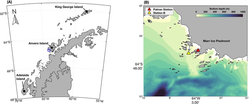
19395590, 0, Downloaded from https://aslopubs.onlinelibrary.wiley.com/doi/10.1002/lno.12314, Wiley Online Library on [05/02/2023]. See the Terms and Conditions (https://onlinelibrary.wiley.com/terms-and-conditions) on Wiley Online Library for rules of use; OA articles are governed by the applicable Creative Commons License
Nardelli et al.                                                                                    WAP coastal phytoplankton seasonal succession

Fig. 1. (A) Map of the West Antarctic Peninsula with the blue box indicating the extents of the Palmer region shown in (B).

filters (pore size = 0.7 μm, diameter = 25 mm), flash-frozen in                  equivalent spherical diameter, area, and biovolume of each
liquid nitrogen, and stored at 80 C for analysis after the field              cell. Processed images were then sorted into 40 taxonomic
season. The samples were shipped to Rutgers University (New                    groups using a medium complexity convolutional neural net-
Brunswick, NJ), where they were run on the HPLC system fol-                    work ( 2,000,000 parameters) that was created and validated
lowing methods in Carvalho et al. (2020). Using the output                     using WAP phytoplankton (Nardelli et al. 2022). Processed
HPLC pigment data, phytoplankton taxonomic composition                         images, along with their predicted identifications, associated
was quantitatively determined in CHEMTAX V1.95 using pig-                      features, and metadata were uploaded to the web application
ment ratios derived from WAP phytoplankton (Kozlowski                          EcoTaxa (Picheral et al. 2017; https://ecotaxa.obs-vlfr.fr),
et al. 2011). Output phytoplankton groups include diatoms,                     where predicted images were manually validated.
cryptophytes, prasinophytes, haptophytes, and mixed flagel-                         Identification of individual cells was performed to the
lates (including both dinoflagellates and other phytoflagel-                     highest possible taxonomic resolution given image resolution,
lates). Although there are alternative methods to quantify                     for example, most diatoms were identified to genus/species
Antarctic Peninsula phytoplankton taxonomic groups from                        level and most phytoflagellates were identified to class level
CHEMTAX data (e.g., Mendes et al. 2018b), we used methods                      (cryptophyte, haptophyte, and prasinophyte; see Table 1),
from Kozlowski et al. (2011) to remain consistent with previ-                  with guidance from Hasle et al. (1997) and Scott and March-
ously published datasets from the PAL-LTER.                                    ant (2005). Mixed flagellates included dinoflagellates
                                                                               (e.g., Gymnodinium spp., Gyrodinium spp., and others),
Phytoplankton species and cell size analysis                                   silicoflagellates (e.g., Dictyochales spp.), and other unidentified
   For species identification and cell size distributions, 5 mL                 phytoflagellates.        Prasinophytes       primarily      included
of each surface sample was analyzed with an Imaging                            Pyramimonas spp. and Pterosperma spp., and haptophytes pri-
FlowCytobot (IFCB; McLane Labs). The IFCB is an imaging-in-                    marily included Phaeocystis antarctica. Diatoms were divided
flow cytometer that uses a combination of imaging and flow                       into centric and pennate groups (see Table 1). Unidentified
cytometric technology to collect images and measure Chl                        centric discoid cells included Thalassiosira spp., Coscinodiscus
a fluorescence and scattered light for each particle ( 10–                     spp., Minidiscus chilensis, Porosira spp., Actinocyclus actinochilus,
150 μm) in each water sample (Olson and Sosik 2007).                           Asteromphalus hookeri, and Stellarima microtrias, among others.
Samples were passed through a 150 μm Nitex screen prior to                     Unidentified pennate cells included Banquisia belgicae,
analysis to prevent large cells from clogging the IFCB’s flow                   Membraneis spp., Navicula spp., Fragilariopsis spp., and
cell. Cells with major axis length < 20 pixels (5.88 μm) were                  Nitzschia spp., among others. Chains of unidentified centric
eliminated from the analysis as the resolution of the images                   and pennate diatom species were included in the > 20 μm
was insufficient to provide clear identification.                                category.
   Images were extracted from IFCB files and processed using                        In addition, aggregated metrics for all phytoplankton cells
methods and software from Sosik and Olson (2007) (https://                     and for the six broad taxonomic groups (centric diatoms, pen-
github.com/hsosik/ifcb-analysis/wiki). Image processing cre-                   nate diatoms, cryptophytes, mixed flagellates, haptophytes,
ates a set of 233 features describing each image including                     and prasinophytes) were calculated for each sample. These

                                                                           3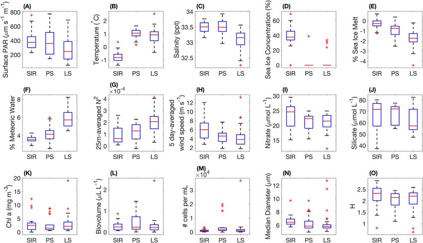
19395590, 0, Downloaded from https://aslopubs.onlinelibrary.wiley.com/doi/10.1002/lno.12314, Wiley Online Library on [05/02/2023]. See the Terms and Conditions (https://onlinelibrary.wiley.com/terms-and-conditions) on Wiley Online Library for rules of use; OA articles are governed by the applicable Creative Commons License
Nardelli et al.                                                                         WAP coastal phytoplankton seasonal succession

Table 1. Median phytoplankton cell size (μm) for each taxonomic group in each successional phase using IFCB data.

                                          Spring ice retreat                     Peak summer                              Late summer
Taxonomic groups                     n             Medianstd             n            Medianstd                    n          Medianstd
Cryptophytes                        9133             8.511.18          10,723          8.671.46                 2305           8.671.71
Mixed flagellates                   18,993            5.812.38          18,933          5.612.05                29,944          5.631.73
Haptophytes                         5695             6.751.99           2253           5.680.75                 3273           5.690.77
Prasinophytes                       3148             8.401.52           1180           7.971.21                  991           8.362.61
Diatoms                            24,164            5.945.32          31,301          5.751.97                20,075          6.193.79
  Centric diatoms                   7026             7.078.86           3097           7.854.05                 5061           12.894.42
    Chaetoceros spp.                545              6.309.81            26            9.776.56                  88            14.679.45
    Corethron pennatum               97             31.0818.76           0                NA                       12          38.8112.15
    Eucampia antarctica              29             43.1814.90           1               84.45                      1             44.05
    Dactyliosolen spp.               9              13.1610.76           0                NA                        3           8.771.16
    Odontella weissflogii             1                 53.29              0                NA                        0              NA
    Probiscia spp.                   7              47.1419.13           3            45.4714.60                 2            45.9413.26
    Unidentified 0–10 μm             4835             6.900.83           2033           6.971.05                 1388           7.130.97
    Unidentified 10–15 μm            716             12.151.31           858           12.531.35                 2609           13.221.19
    Unidentified 15–20 μm            217              16.061.21          150           16.061.11                  874           15.911.03
    Unidentified > 20 μm             570             39.8720.92          26            27.729.96                  84            29.779.43
  Pennate diatoms                  17,138            5.572.58          28,204          5.671.12                15,014          5.811.97
    Amphiprora spp.                  46             16.984.51             0               NA                       0                NA
    Cocconeis spp.                   4              14.253.45            13           12.057.47                   25           12.843.83
    Cylindrotheca spp.              228              9.812.14            1               10.84                      6           9.060.75
    Licmophora spp.                  7              16.156.46            16           15.494.73                  19            14.566.86
    Pseudo-nitzschia spp. chains    371             14.733.74            15           12.032.71                  113           14.124.21
    Unidentified 0–10 μm            15,987            5.510.92          27,955          5.660.72                14,227          5.751.12
    Unidentified 10–15 μm            352             11.171.20           168           11.081.14                  573           10.971.13
    Unidentified 15–20 μm             58             17.721.41           13            16.341.52                  34            17.451.47
    Unidentified > 20 μm              85             24.776.64            23           24.885.04                   17           25.035.27

include total biovolume (sum biovolume of all cells in a sam-         in 2018–2019, samples were preserved on 13 December and
ple divided by the mL of water sampled), total abundance              from 07 January to 28 March. On 22, 26, and 28 December
(total number of cells in a sample divided by the mL of water         2017, live samples were collected alongside preserved samples
sampled), and median cell diameter.                                   for comparison. On average, total biovolume and cell abun-
   Since IFCB-derived phytoplankton biovolume and HPLC-               dance of preserved samples were underestimated by 48.07%
derived Chl a concentrations were both estimates of total phy-        and 36.36%, respectively, when compared to live samples
toplankton biomass for each method, we compared the two               (Fig. S2A,B). However, relative changes in biovolume and
using Kendall rank correlation to confirm general agreement.           abundance were similar between the three samples
To validate taxonomic precision, IFCB data were separated             (Fig. S2A,B), as were the relative percentages of different taxo-
into broad taxonomic groups matching those derived from               nomic groups (Fig. S2C–E). Cryptophytes and prasinophytes
HPLC (diatoms, cryptophytes, prasinophytes, haptophytes,              were consistently found at higher percentages in preserved
mixed flagellates). Then, the methods were compared for each           vs. live samples, indicating a potential preservation bias
taxonomic group by evaluating the Kendall rank correlation            toward these groups (on average 17.38% more cryptophytes
between percent taxa in each sample for both methods.                 and 32.86% more prasinophytes in preserved samples;
   In both years, preserved samples (5 mL whole seawater in           Fig. S2C–E).
50% glutaraldehyde) were collected during times when the                 To quantify phytoplankton diversity from IFCB data, the
IFCB was not available (i.e., undergoing maintenance or               Shannon diversity index (H) was used, which describes the
aboard the vessel on the annual 1-month WAP cruise).                  number and richness of groups sampled:
Fixed samples were flash-frozen in liquid nitrogen and stored                                          X
                                                                                                      R
at 80 C for analysis after the field season. In 2017–2018,                                    H ¼         pi ln pi ,
samples were preserved from 05 January to 05 February, and                                            i¼1

                                                                  4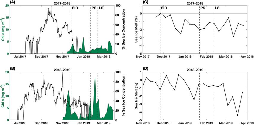
19395590, 0, Downloaded from https://aslopubs.onlinelibrary.wiley.com/doi/10.1002/lno.12314, Wiley Online Library on [05/02/2023]. See the Terms and Conditions (https://onlinelibrary.wiley.com/terms-and-conditions) on Wiley Online Library for rules of use; OA articles are governed by the applicable Creative Commons License
Nardelli et al.                                                                            WAP coastal phytoplankton seasonal succession

where pi is the proportion of individuals in the ith group iden-        at Columbia University (New York, NY), where they were
tified in the dataset and R is the total number of groups identi-        analyzed following methods in Carvalho et al. (2020).
fied in the data set. Higher values of H suggest that there are             Mixed layer depths could not be confidently predicted
both more groups represented in the data set and more mem-              (QI < 0.5; Lorbacher et al. 2006) at Sta. B due to the shallow
bers of each of those groups. An H value of zero indicates only         water depth ( 60 m). Thus, mean Brunt–Väisälä frequency
one group present in the dataset.                                       (N2) values were calculated for the top 25 m using methods
                                                                        from Carvalho et al. (2017) to quantify and compare upper
Ancillary data                                                          water-column stability within and between our two sampling
    Sea ice metrics were calculated from satellite-derived daily        years.
sea ice concentration (%) data determined using the GSFC                   Wind speed (m s1; RM Young, Model 05108-45) and pho-
Bootstrap algorithm version 3.1 and extracted for the                   tosynthetically active radiation (PAR; μmol s1 m1; Licor,
25 km  25 km satellite pixel closest to Palmer Station. Fol-           Model LI 190) measurements were obtained from an auto-
lowing methods in Stammerjohn et al. (2008), day of ice-edge            mated weather station located just behind Palmer Station.
advance was calculated as the first day when sea ice concentra-          Five-day means of wind speed (current day and the four previ-
tion exceeded a 15% threshold for at least 5 consecutive days;          ous days) and daily mean PAR were calculated from
day of ice-edge retreat was calculated as the last day before sea       2-min data.
ice concentration dropped below a 15% threshold after being
above 15% for at least 5 consecutive days; sea ice duration is          Statistical analyses
the number of days between the day of advance and the day                   One-way analysis of variances with Kruskal–Wallis post hoc
of retreat, and number of sea ice days are the number of days           tests were conducted for each environmental variable (sea ice
between the day of advance and day of retreat where sea ice             concentration, PAR, surface temperature, surface salinity, per-
concentration is > 15%.                                                 cent meteoric water, percent sea ice meltwater, N2, wind
    Meltwater composition was derived from oxygen isotope               speed, nitrate, phosphate, and silicate) and phytoplankton
composition (δ18O) once per week. Water from each surface               variable (Chl a concentration, H, and IFCB-derived phyto-
sample was drawn into a 50 mL glass vial, sealed with a stop-           plankton biovolume, abundance, and median diameter), to
per and aluminum crimp, and stored in a dark, +4 C box.                determine whether values were significantly different between
Samples were transported to the National Environmental Iso-             the two field seasons.
tope Facility at the British Geological Survey (Keyworth, Not-              To assess relationships between environmental and phyto-
tinghamshire, UK). There, an Isoprime 100 mass spectrometer             plankton variables, we conducted a principal components analy-
plus Aquaprep device were used to analyze δ18O using the                sis (PCA) on all data from both years, using z-scores from
CO2 equilibration method. Measurements were calibrated                  environmental (sea ice concentration, PAR, surface temperature,
against internal and international standards (e.g., VSMOW2              surface salinity, percent meteoric water, percent sea ice meltwa-
and VSLAP2). An analytical reproducibility of  0.02‰ was               ter, N2, wind speed, nitrate, and silicate) and phytoplankton
obtained with duplicate analysis. Using δ18O and surface salin-         (percent biovolume attributed to centric diatoms, pennate dia-
ity data, we quantitatively separated sea ice melt from mete-           toms, cryptophytes, mixed flagellates, prasinophytes, and
oric water (glacial melt, precipitation, and runoff from snow           haptophytes) variables. Linear interpolation was used to fill in
melt) by solving a three-endmember mass balance equation                missing values in the environmental data—this included 7 values
(see methods and endmember values in Meredith et al. 2021).             in the nitrate and silicate data, and 39 values in the percent
Using this mass balance equation, negative values for sea ice           meteoric water and sea ice melt data over both seasons (δ18O
melt are possible and are indicative of net sea ice formation           was only sampled once per week). Using a k-means cluster analy-
(i.e., more sea ice grew in situ than melted in situ due to lat-        sis on the same dataset, a silhouette test identified three clusters
eral advection). Glacial meltwater discharge is a dominant              representing successional phases: a Spring Ice Retreat Phase, a
meteoric source in the coastal and nearshore regions of the             Peak Summer Phase, and a Late Summer Phase. Kendall rank cor-
WAP (Meredith et al. 2013, 2017, 2021), but here we will con-           relation tests were used to quantify relationships found in the
tinue to refer to this derived metric as “meteoric water” to            PCA. Nonparametric statistics were used due to the non-normal
explicitly reflect the fact that it comprises both precipitation         data distributions for most variables.
and glacial meltwater inputs.
    Surface samples were analyzed for nitrate plus nitrite
(NO3 + NO2; hereafter called nitrate due to the very low              Results
concentration of nitrite), phosphate (PO43), and silicate              HPLC vs. IFCB taxonomy comparison
(Si[OH]4). Each surface sample (1 L) was filtered through                  HPLC-derived Chl a concentrations were significantly posi-
GF/F filters (pore size = 0.7 μm, diameter = 25 mm) and stored           tively correlated to IFCB-derived biovolume concentrations
at 20 C in 15 mL acid-rinsed Falcon centrifuge tubes. The             (Fig. S3). The two methods yielded similar timing and magni-
samples were shipped to Lamont Doherty Earth Observatory                tude of biomass peaks within each field season, with notable

                                                                    5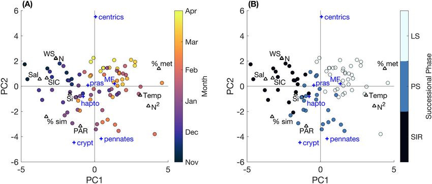
19395590, 0, Downloaded from https://aslopubs.onlinelibrary.wiley.com/doi/10.1002/lno.12314, Wiley Online Library on [05/02/2023]. See the Terms and Conditions (https://onlinelibrary.wiley.com/terms-and-conditions) on Wiley Online Library for rules of use; OA articles are governed by the applicable Creative Commons License
Nardelli et al.                                                                                WAP coastal phytoplankton seasonal succession

Fig. 2. Spring to autumn (A and B) HPLC-derived chlorophyll a and (C and D) IFCB-derived biovolume for each phytoplankton group. Pie chart insets
show total percent (A and B) chlorophyll a or (C and D) biovolume for each group over the entire field season. Gray areas in plots C and D indicate
periods when IFCB results are based on preserved samples. Vertical dashed lines indicate the overall mean date of each seasonal succession phase
(SIR = Spring Ice Retreat Phase, PS = Peak Summer Phase, and LS = Late Summer Phase).

differences including much lower relative peaks for IFCB-                   (138 d in 2017 vs. 178 d in 2018), and less total sea ice days
derived biovolume on 19 November 2018 and 21 January                        (125 d in 2017 vs. 177 d in 2018; Fig. 3A,B). Sea ice was rap-
2019 compared to HPLC-derived Chl a (Fig. 2).                               idly advected from the region in 2017, dropping from 49% on
    In addition, there were significant, positive correlations               27 November to 0% on 03 December (Fig. 3A). In 2018, there
between percent taxa calculated with each method for dia-                   was an initial drop in sea ice concentration from 96% on
toms, cryptophytes, prasinophytes, and mixed flagellates                     02 November to 29% on 05 November, but sea ice remained
(Fig. S4A–D), and a nonsignificant, positive correlation for                 steady at an average of 34.8% until it retreated on
haptophytes (Fig. S4E). However, IFCB classification over-                   26 December, with intermittent advection in and out of the
predicted mixed flagellates compared to HPLC classification,                  region until 16 January (Fig. 3B).
illustrated by the skew of points above the 1 : 1 line in                      Consistent with rapid advection, there were no positive sea
Fig. S4D, and by the greater total percent of mixed flagellates              ice melt contributions to coastal surface waters in 2017
classified by the IFCB than by HPLC for the entire field season               (Fig. 3C), while there were significant positive contributions
(23% greater in 2017–2018 and 7% greater in 2018–2019;                      in November and December in 2018 (Fig. 3D). δ18O-derived
Fig. 2). Similarly, IFCB classification underpredicted diatoms               freshwater sources (sea ice melt and meteoric water) reflect the
compared to HPLC classification, illustrated by the skew of                  net seasonal freshwater balance, so negative values of percent
points below the 1 : 1 line in Fig. S4A, and by the lesser total            sea ice melt indicate that seasonally, there was net sea ice
percent of diatoms classified by the IFCB than by HPLC for                   growth in the Palmer region (i.e., more sea ice grew here than
the entire field season (24% lesser in 2017–2018 and 8% lesser               melted here). Thus, negative values in November and
in 2018–2019; Fig. 2). Despite discrepancies between methods,               December 2017 likely indicate that sea ice was grown in the
IFCB data provided information that HPLC data could not,                    Palmer region the previous autumn–winter and melted else-
including cell size and species composition within taxonomic                where in spring, whereas positive values in December and
groups (Table 1).                                                           January 2018 indicate local spring melting that exceeds the
                                                                            previous autumn–winter local growth. During the sampling
Interannual differences                                                     period (01 November–31 March), sea ice concentrations were
   Compared to the winter of 2018, the winter of 2017 had a                 significantly higher in 2018–2019 than in 2017–2018
later fall sea ice-edge advance date (17 July 2017 vs. 01 July              (Table S1). Aside from interannual differences in sea ice due to
2018), an earlier spring sea ice-edge retreat date (02 December             wind-driven advection, the physical and biogeochemical envi-
2017 vs. 26 December 2018), shorter sea ice season duration                 ronments were relatively similar between the 2 yr, except for

                                                                        6
19395590, 0, Downloaded from https://aslopubs.onlinelibrary.wiley.com/doi/10.1002/lno.12314, Wiley Online Library on [05/02/2023]. See the Terms and Conditions (https://onlinelibrary.wiley.com/terms-and-conditions) on Wiley Online Library for rules of use; OA articles are governed by the applicable Creative Commons License
Nardelli et al. WAP coastal phytoplankton seasonal succession
Fig. 3. Spring to autumn (A and B) chlorophyll a concentration (green) overlaid with daily percent sea ice concentration (black line) for (A) 2017–2018
and (B) 2018–2019. Percent sea ice melt for (C) 2017–2018 and (D) 2018–2019, where positive values indicate net seasonal sea ice melt and negative
values indicate net seasonal sea ice formation. Vertical dashed lines indicate the overall mean date of each seasonal succession phase (SIR = Spring Ice
Retreat Phase, PS = Peak Summer Phase, and LS = Late Summer Phase).
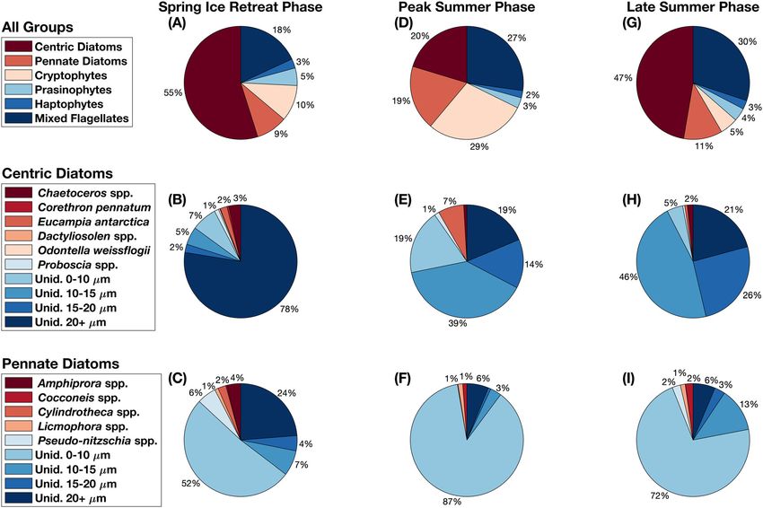
higher temperatures in 2017–2018, and higher concentrations season occurred. This Spring Ice Retreat Phase bloom contained
of nitrate and silicate in 2018–2019 (Table S1). the highest diversity of the season (Fig. 5O) and was comprised
Phytoplankton data showed significantly higher Chl of high centric diatom abundance (55% of total biovolume), and
a concentrations in 2018–2019, but significantly lower comparatively high seasonal prasinophyte (5% total biovolume,
H values indicating fewer species and less evenness in species mainly Pyramimonas spp.) and haptophyte abundances (3% total
abundance (Table S2). Taxonomically, there were greater per- biovolume, mainly P. antarctica; Fig. 6A; Table 1). These centric
cent diatom and haptophyte biovolumes in 2018–2019, and diatoms were 78% unidentified discoid cells with diameters
greater percent mixed flagellate and prasinophyte biovolumes > 20 μm, likely consisting of a mix of large, chain-forming dia-
in 2017–2018 (Fig. 2 pie charts; Table S3). toms including Thalassiosira spp. (Fig. 6B). Centric diatom species
including Chaetoceros spp., C. pennatum, and Eucampia antarctica,
Spring–autumn successional trends and pennate diatom species including Amphiprora spp.,
PCA results showed seasonal changes in the environment Cylindrotheca spp., and Pseudo-nitzschia spp. chains had their
that were reflected in phytoplankton successional changes highest cell counts during this phase (Table 1).
averaged over both field seasons (Fig. 4). The three calculated The Peak Summer Phase was a transition phase character-
clusters occurred sequentially in time, with cluster 1 (Spring ized by relatively high surface temperatures (mean = 1.0 C)
Ice Retreat Phase) centered at 26 November, cluster 2 (Peak and surface salinities (mean = 33.5 ppt), low wind speeds
Summer Phase) centered at 22 January, and cluster 3 (Late (mean = 4.3 m s1) and moderate water column stability
Summer Phase) centered at 12 February (Fig. 4; Table S5). See (mean = 1.2 104), less sea ice melt (mean = 0.9%) but
Figs. S5–S8 for the full timeseries of each dataset. higher meteoric water percentages (mean = 4.2%), lower nutri-
Compared to the other two phases, the Spring Ice Retreat ent concentrations (mean nitrate = 21.1 μmol L1, mean
Phase was characterized by relatively high sea ice concentrations phosphate = 1.6 μmol L1, and mean silicate = 67.0 μmol L1),
(mean = 39%) and sea ice melt (mean = 0.3%), high wind and high but variable PAR (mean = 399.7 μm s1 m1; Fig. 5;
speeds (mean = 6.1 m s1) and corresponding lower water col- Table S5). Sea ice concentrations were negligible during this
umn stability (mean = 9.2 105), high nutrient concentrations phase (mean = 1.8%; Fig. 5D; Table S5). The Peak Summer
(mean nitrate = 23.5 μmol L1, mean phosphate = 1.7 μmol L1, Phase had the lowest Chl a concentrations but highest IFCB-
and mean silicate = 67.1 μmol L1), cold surface water tempera- derived biovolume and abundance values, and the lowest phy-
tures (mean = 0.7 C) and high surface water salinities toplankton diversity of the season (Fig. 5K–M,O). The Peak
(mean = 33.5 ppt; Fig. 5; Table S5). As sea ice concentrations Summer Phase was associated with high cryptophyte abun-
dropped below 50% in November, the first bloom of the dance (29% total biovolume), mixed flagellate abundance (27%
719395590, 0, Downloaded from https://aslopubs.onlinelibrary.wiley.com/doi/10.1002/lno.12314, Wiley Online Library on [05/02/2023]. See the Terms and Conditions (https://onlinelibrary.wiley.com/terms-and-conditions) on Wiley Online Library for rules of use; OA articles are governed by the applicable Creative Commons License
Nardelli et al. WAP coastal phytoplankton seasonal succession
Fig. 4. PCA results showing loadings: triangles for environmental variables (Temp = temperature, Sal = salinity, WS = wind speed, SIC = sea ice concen-
tration, % sim = % sea ice melt, % met = % meteoric water, N = nitrate, and Si = silicate) and + for phytoplankton variables (centrics = centric diatoms,
pennates = pennate diatoms, crypt = cryptophytes, MF = mixed flagellates, pras = prasinophytes, and hapto = haptophytes), with values multiplied by
10 for readability; and circles represent the coordinate for each sample based on the magnitude of PC1 and PC2 and in (A) are color coded by date, and
in (B) are color coded by the three successional phases determined by k-means clustering (SIR = Spring Ice Retreat Phase, PS = Peak Summer Phase,
LS = Late Summer Phase). The first two principal components represent 24.5% variance and 14.16% variance, respectively.
Fig. 5. Boxplots showing aggregated (A–J) environmental and (K–O) phytoplankton data over the 2 yr for the three successional phases: Spring Ice
Retreat Phase (SIR), Peak Summer Phase (PS), and Late Summer Phase (LS). In each box plot, the horizontal red line represents the median value, the top
and bottom box limits represent the 25th and 75th percentiles, whiskers represent the full range of non-outlier observations, and red + symbols represent
outliers.
819395590, 0, Downloaded from https://aslopubs.onlinelibrary.wiley.com/doi/10.1002/lno.12314, Wiley Online Library on [05/02/2023]. See the Terms and Conditions (https://onlinelibrary.wiley.com/terms-and-conditions) on Wiley Online Library for rules of use; OA articles are governed by the applicable Creative Commons License
Nardelli et al. WAP coastal phytoplankton seasonal succession
Fig. 6. Percent biovolume for (A, D, G) all taxonomic groups, (B, E, H) centric diatoms and (C, F, I) pennate diatoms during the (A–C) Spring Ice
Retreat Phase, (D–F) Peak Summer Phase, and (G–I) Late Summer Phase. Data are aggregated over both years for each phase. The percentage labels for
groups with values < 1% were not included. Unid. = Unidentified.
total biovolume), and pennate diatom abundance (19% of total (mean = 33.1 ppt), highest meteoric water percentages
biovolume; Fig. 6D; Table 1). The pennate diatom community (mean = 5.9%), highest water column stability (mean =
was 87% comprised of unidentified cells with diameters 2.0 104), low but variable wind speeds (mean = 4.3 m s1),
< 10 μm (likely including Fragilariopsis spp. and Nitzschia spp.; and low nutrient concentrations (mean nitrate = 21.3
Fig. 6F). μmol L1, mean phosphate = 1.5 μmol L1, and mean
The Peak Summer Phase pennate diatom community was silicate = 61.9 μmol L1; Fig. 5; Table S5). Sea ice concentra-
especially prevalent in early February 2019 (relative to 2018), tions were negligible during this phase (mean = 3.2%;
when there was a large pennate diatom bloom associated with Fig. 5D). The Late Summer Phase was associated with rela-
high water column stability (peak biovolume of 2.43 μL L1 on tively high centric diatom abundance (47% total biovolume)
4 February; Fig. 2). A wind event from 25 January to 28 January and mixed flagellate abundance (30% total biovolume;
(mean 5.34 m s1) co-occurred with a drop in N2, a peak in Fig. 6G; Table 1). Of the centric diatoms, 46% were uni-
salinity, a drop in percent meteoric water, and a peak in nutri- dentified discoid cells with a diameter between 10 and 15 μm
ents (Figs. S5F,H,J,L, S6B,D,F). Just after this wind event, surface and 26% were unidentified discoid cells with a diameter
PAR increased dramatically and wind speeds dropped, causing between 15 and 20 μm (likely including smaller Thalassiosira
percent meteoric water to peak on 04 February corresponding spp. and M. chilensis; Fig. 6H). Pennate diatom species includ-
with a dramatic dip in surface temperature, and the lowest ing Cocconeis spp. and Licmophora spp. had their highest cell
salinity, highest N2 value, highest Chl a value, and lowest counts during this phase (Table 1).
nutrient concentrations of the field season (Figs. S5B,D,F,H,J,L, Matching seasonal succession patterns, phytoplankton
S6B,D,F). median cell size decreased during both field seasons (Figs. 5N,
The Late Summer Phase was characterized by relatively S9). This trend was positively correlated with a decrease in
lower but variable PAR (mean = 282.5 μm s1 m1), high sur- salinity from spring to autumn during both field seasons
face temperatures (mean = 0.9 C), the lowest surface salinities (Kendall; 2017–2018: p = 9.45 104 and τ = 0.38; 2018–
919395590, 0, Downloaded from https://aslopubs.onlinelibrary.wiley.com/doi/10.1002/lno.12314, Wiley Online Library on [05/02/2023]. See the Terms and Conditions (https://onlinelibrary.wiley.com/terms-and-conditions) on Wiley Online Library for rules of use; OA articles are governed by the applicable Creative Commons License
Nardelli et al. WAP coastal phytoplankton seasonal succession
2019: p = 0.04 and τ = 0.22), suggesting increasing freshwater spring (September–October) can precondition the water column
might be responsible for the decrease in cell size. Surface salin- due to its effect on sea ice and consequently percent sea ice
ity, percent meteoric water, and upper water-column stability melt, which in turn could either serve to enhance (as in 2018–
were tightly linked during both years (Fig. 4), with low salinity 2019) or dampen (2017–2018) surface freshening and stratifica-
corresponding to high percent meteoric water (Kendall; 2017– tion, influencing phytoplankton biomass and species composi-
2018: p = 2.38 105 and τ = 0.66; 2018–2019: tion. Although the spring ice-edge retreated later in 2018–2019
p = 1.88 105 and τ = 0.62) and high N2 values (Kendall; than in 2017–2018 (26 December vs. 03 December), the initial
2017–2018: p = 4.61 1012 and τ = 0.70; 2018–2019: phytoplankton bloom occurred earlier due to relatively low
p = 2.75 1012 and τ = 0.67). Higher N2 values were also ( 30%) sea ice coverage starting in early November, allowing
correlated with lower wind speeds (Kendall; 2017–2018: adequate light for phytoplankton growth. Sea ice then slowly
p = 3.83 104 and τ = 0.39; 2018–2019: p = 4.93 106 melted through mid-January, further enhancing surface stratifi-
and τ = 0.47), while higher nitrate concentrations were corre- cation and stabilizing the upper water column, conditions opti-
lated with higher wind speeds (Kendall; 2017–2018: p = 0.03 mal for phytoplankton growth that in turn contributed to
and τ = 0.24; 2018–2019: p = 0.01 and τ = 0.30; Fig. 4). significantly higher Chl a concentrations in 2018–2019 (Rozema
et al. 2017). In contrast, in 2017, there was > 50% sea ice cover-
age through most of November, likely inhibiting light penetra-
Discussion
tion and subsequent phytoplankton growth. Dramatic reduction
This work reveals the mechanisms of winter sea ice dynam- in sea ice coverage at the end of November indicates rapid,
ics influencing interannual phytoplankton biomass and dia- wind-driven advection of sea ice from the region, leading to neg-
tom abundance, as well as the importance of meteoric water ative sea ice melt percentages near Palmer Station and allowing
in structuring water column stability later in the summer sea- high variability in N2, likely contributing to the significantly
son in tandem with a shift toward smaller phytoplankton cell lower Chl a concentrations seen during this field season
sizes (e.g., pennate diatoms < 10 μm). Despite significant dif- (Rozema et al. 2017).
ferences in sea ice extent and total phytoplankton biomass It is possible that with rapid wind-driven advection of sea
between years, phytoplankton successional patterns were ice from the region in 2017, less sea ice algae were released to
remarkably similar and driven by consistent seasonal drivers seed the coastal region near Palmer Station. This can be com-
(e.g., solar irradiance, temperature, and freshwater inputs), pared to 2018 when sea ice lingered and contributed more
while storm/wind events drove more ephemeral differences meltwater and potentially more seed populations, with higher
between years (e.g., the early February 2019 event). Phyto- associated Chl a concentrations in 2018–2019 than in 2017–
plankton species composition and cell size information col- 2018 (Ackley and Sullivan 1994; van Leeuwe et al. 2018). Ear-
lected by the IFCB was invaluable for gaining this more in- lier sea ice advance in the autumn is expected to entrain
depth understanding of seasonal and interannual phytoplank- higher concentrations of algae, therefore, the 16 d earlier sea
ton dynamics at Palmer Station. ice advance in autumn 2018 might also have contributed to
increased phytoplankton concentrations in the 2018–2019
Drivers of interannual phytoplankton differences field season (Garrison et al. 1983).
Along the WAP, phytoplankton demonstrate strong inter- Silicate and nitrate were found at significantly higher con-
annual and regional variability, seasonally timed with light centrations in 2018–2019 than in 2017–2018. Typically, years
availability and spring sea ice retreat. As day length increases with reduced sea ice and higher wind-driven mixing lead to
in austral spring, solar warming and sea ice melt help to stabi- higher nutrient injection into surface waters from deeper,
lize the upper water column allowing phytoplankton to nutrient-rich waters (Annett et al. 2010). Following this logic,
remain near the surface in waters with higher light availability we would expect to see higher nutrient concentrations in
(Vernet et al. 2008; Venables et al. 2013). These conditions ini- 2017–2018. However, there were faster wind speeds at the
tiate large diatom-dominated spring blooms (Mitchell and start of the growing season in 2018 (Spring Ice Retreat Phase
Holm-Hansen 1991; Prézelin et al. 2000) as we saw in both mean = 6.5 m s1) than in 2017 (Spring Ice Retreat Phase
field seasons. Similar to other studies, we found that both lon- mean = 5.0 m s1) that could have contributed to higher ini-
ger winter sea ice durations (Saba et al. 2014; Rozema tial concentrations. In addition, there were much larger nutri-
et al. 2017; Schofield et al. 2017) and a slower rate of ice-edge ent drawdown events by high biomass blooms in 2018–2019
retreat in spring to early summer (Garibotti et al. 2005a; than in 2017–2018 that would be expected to lower seasonal
Annett et al. 2010; Gonçalves-Araujo et al. 2015) contributed nutrient concentrations, emphasizing that wind-driven
to high phytoplankton abundance and a diatom-dominated mixing must have more than compensated for the larger
community. nutrient drawdown in 2018–2019 (Fig. S5K,L).
Winter sea ice duration was 40 d shorter in 2017 than in Taxonomically, there were proportionally more mixed fla-
2018, and the phytoplankton community had less diatoms gellates and prasinophytes in 2017–2018 and proportionally
and more mixed flagellates. Wind speed and direction in early more diatoms and haptophytes in 2018–2019. Dominance of
1019395590, 0, Downloaded from https://aslopubs.onlinelibrary.wiley.com/doi/10.1002/lno.12314, Wiley Online Library on [05/02/2023]. See the Terms and Conditions (https://onlinelibrary.wiley.com/terms-and-conditions) on Wiley Online Library for rules of use; OA articles are governed by the applicable Creative Commons License
Nardelli et al. WAP coastal phytoplankton seasonal succession
diatoms and haptophytes (e.g., P. antarctica) has been associ- where they can supplement photosynthesis with phagotrophy
ated with the marginal sea ice zone (Garibotti et al. 2005a), (Goes et al. 2014). However, we saw an increase in surface
which could explain why we saw higher proportions of both water biomass during the Peak Summer Phase when PAR and
in 2018–2019. Low light environments (e.g., deep mixed layer temperature were high, matching other regional studies (Biggs
depths) have been found to favor mixed flagellates (Schofield et al. 2019; Pan et al. 2020). High-light environments could
et al. 2017; Carvalho et al. 2020), thus a significantly higher give mixotrophs a competitive advantage over heterotrophs,
proportion of mixed flagellates in 2017–2018 may be related as they can supplement their carbon supply with photosyn-
to variable N2 during that field season. In addition, there was thesis (Edwards 2019). In addition, cryptophytes are especially
higher overall community diversity in 2017–2018, as large dia- well-adapted to high-light environments due to specialized
tom blooms in 2018–2019 were dominated by only a few tax- protective pigments (Mendes et al. 2018a). Contrary to other
onomic groups. This finding was unexpected, as Lin et al. WAP studies (Moline et al. 2004; Schofield et al. 2017; Mendes
(2021) found less diverse phytoplankton assemblages associ- et al. 2018a), we did not find significant correlations between
ated with higher sea surface temperatures, deeper mixed cryptophytes and low salinity, macronutrients, or percent
layers, and low sea ice extent along the WAP. Water column meteoric water. Thus, it is likely that biotic successional pat-
stability was not significantly different between our two study terns drove this rise in cryptophytes rather than specific abi-
years, so it is possible that analyzing additional years with sig- otic environmental drivers.
nificantly different physical conditions may elicit the patterns In 2018–2019, the Peak Summer Phase also had a very
seen by Lin et al. (2021). large, stability-induced pennate diatom bloom, likely com-
prised of Fragilariopsis spp. and Nitzschia spp. This bloom had
Drivers of phytoplankton seasonal succession almost twice as much biomass as any other bloom seen over
Following phytoplankton trends found in previous years both field seasons, possibly because the wind event that pre-
near Palmer Station (Garibotti et al. 2005a; Schofield ceded the bloom resuspended iron as well as macronutrients,
et al. 2017), we confirmed three distinct successional phases and because smaller diatoms have both high maximum
in both field seasons despite variability in the environmental growth rates and an enhanced ability to accelerate growth
drivers: a Spring Ice Retreat Phase dominated by large-celled rates (Behrenfeld et al. 2021). This bloom of small pennate
diatoms, followed by a Peak Summer Phase dominated by diatoms also co-occurred with a pulse of meteoric water and
cryptophytes, followed by a Late Summer Phase dominated by increased surface stratification (i.e., very high N2), which has
small-celled diatoms. The phytoplankton growing season is been observed in other field studies (Beans et al. 2008; Höfer
initiated during the Spring Ice Retreat Phase as solar irradiance et al. 2019; Pan et al. 2020). An experimental study by
increases (Venables et al. 2013). Matching our results, van Hernando et al. (2015) using phytoplankton from Potter Cove,
Leeuwe et al. (2022) found two ice-associated phytoplankton Antarctica found that low salinity conditions (30 PSU)
phases: an initial phase of flagellates such as Pyramimonas spp. increased the proportion of small pennate diatoms ( 0% on
and P. antarctica caused by seeding during sea ice melt (which day 4 to 95% on day 8) and decreased the proportion of
we saw in higher relative abundance during the Spring Ice large centric diatoms ( 90% on day 2 to 0% on day 7), and
Retreat Phase), followed by an increase in large centric dia- hypothesized that this was due to differing osmotic stress tol-
toms, such as Thalassiosira spp. and Chaetoceros spp., which erances. Meteoric water can also carry micronutrients (Annett
are not present within the sea ice but thrive as the upper water et al. 2017) that can influence species selection and growth
column stratifies providing optimal light conditions. This rates, however, micronutrients were not measured in our
large, stability-induced spring centric diatom bloom has been study. Thus, the pulse of meteoric water during this bloom
seen in other Antarctic studies (Garibotti et al. 2005a,b; Costa could have selected for small pennate diatoms with high
et al. 2020, 2021) and Arctic studies (Lafond et al. 2019; growth rates.
Ardyna et al. 2020). Overall growth conditions are maximized During the Late Summer Phase, increases in wind-driven
in years with protracted sea ice retreat (Annett et al. 2010), mixing replenished nutrients (including iron) to surface
when greater local sea ice melt enhances surface stratification waters and allowed for small diatoms (typically 10–20 μm cen-
and promotes phytoplankton growth, illustrated by higher tric diatoms) to bloom. Previous studies show that iron con-
peak biomass and a greater proportion of large, centric dia- centrations are important for shifting phytoplankton
toms seen in 2018 compared to 2017. composition from a phytoflagellate-dominated community to
Because the large diatom bloom during the Spring Ice a diatom-dominated community (Boyd et al. 2000). In the
Retreat Phase reduced nutrient concentrations, the next suc- Palmer region, iron supply primarily comes from shallow sedi-
cessional phase (Peak Summer Phase) favors mixotrophic phy- ments delivered to surface waters by wind-driven vertical
toplankton such as cryptophytes (Gast et al. 2014; Trefault mixing (Sherrell et al. 2018). We did not sample iron in this
et al. 2021), that can both photosynthesize and consume par- study, but previously collected seasonal data in the Palmer
ticulate organic matter amassed over earlier bloom phases. region showed a six-fold increase from late-January to mid-
Cryptophytes are often found in deeper, low-light conditions February with increases in wind speed and a deepened mixed
1119395590, 0, Downloaded from https://aslopubs.onlinelibrary.wiley.com/doi/10.1002/lno.12314, Wiley Online Library on [05/02/2023]. See the Terms and Conditions (https://onlinelibrary.wiley.com/terms-and-conditions) on Wiley Online Library for rules of use; OA articles are governed by the applicable Creative Commons License
Nardelli et al. WAP coastal phytoplankton seasonal succession
layer depth (Carvalho et al. 2016), which matches the timing In our IFCB samples, we excluded all cells with a major axis
of this phase. The Late Summer Phase is characterized by vari- length less than 20 pixels (5.88 μm) prior to analysis, as these
able mixed layer depths (as inferred from 25 m-averaged N2), small cells are below the quantifiable limit of detection based
driven by contrasting increases in wind speed and meteoric on instrument resolution, and thus have a high probability of
water inputs. These variable conditions may limit the duration being misclassified. P. antarctica is mostly found in the flagel-
and magnitude of this small diatom bloom. Instead, higher late stage during summer in the WAP region below 64 S, with
wind-mixing and decreasing daylength in the late summer cell diameters < 5 μm (Kozlowski et al. 2011; Biggs et al. 2019).
could select for species that do well in turbulent, low-light Since P. antarctica is the dominant haptophyte in our region
environments, resulting in the increased proportion of mixed (Annett et al. 2010), IFCB methods likely underestimated
flagellates that we found (Schofield et al. 2017; Carvalho haptophyte abundances with the exclusion of cells < 5.88 μm,
et al. 2020). leading to the nonsignificant relationship found between IFCB
Over the course of both field seasons, we observed decreas- and HPLC-estimated haptophyte percent composition. This
ing median cell diameter associated with increasing percent also could be the reason for the slight overprediction of
meteoric water and decreasing salinity. Stronger surface strati- prasinophytes using HPLC compared to IFCB, and thus the
fication due to increased freshwater inputs can reduce nutri- weaker correlation between the two methods (Garibotti
ents in surface waters, giving an advantage to smaller et al. 2003).
phytoplankton with high surface-area-to-volume ratios and There were a few notable discrepancies in overall abun-
reduced sinking rates (Li et al. 2009). However, macronutri- dance between the two methods, particularly on 19 November
ents do not appear to be limiting in either field season, and 2018 and 21 January 2019, where HPLC showed peaks in Chl
ratios of Si : N > 2 also suggest no significant limitation by a that were absent or lessened when portrayed by IFCB
iron or other micronutrients (Clarke et al. 2008). As men- biovolume. This discrepancy may not be an error in method-
tioned above, increased meteoric water inputs could cause cell ology and could instead reflect high Chl a to biovolume ratios
size and composition shifts via differing tolerances to low during these 2 d. However, a potential source of error could be
salinity, especially for diatoms (Hernando et al. 2015), and via classification within “detritus” and “multiple” categories. Phy-
micronutrient inputs (Annett et al. 2017). Since diatoms toplankton cells were commonly seen attached to detritus par-
contributed the highest annual percent composition to the ticles, or in large conglomerations. These images were
population in low (44% in 2017–2018) and high (66% in eliminated from the analysis as they could not be reliably
2018–2019) Chl a years, cell size shifts in diatoms have a large sorted into a single taxonomic group. Although it is possible
contribution to the decreasing spring to autumn trend seen in that excluding these groups reduced the biovolume in some
overall phytoplankton cell size. samples, this does not seem to be the case for the days in
question, as total biovolume including non-phytoplankton
HPLC vs. IFCB-derived abundance and taxonomy particles was still very low (see fig. 2 in Nardelli et al. 2022).
In general, HPLC and IFCB-derived biomass and percent Although both peaks were dominated by centric diatoms
taxa estimates agreed. There were positive, significant correla- which typically have diameters > 10 μm in this region (Annett
tions between overall biomass for the two methods and for all et al. 2010), there are some species with diameters < 5.88 μm
taxonomic groups except haptophytes. Similar to other WAP (e.g., M. chilensis), therefore the size cut-off could be responsi-
studies (Kozlowski et al. 2011), the strongest relationships ble for this difference between methods. The absent 21 January
between HPLC and imaging (e.g., IFCB and microscopy) 2019 peak could also be the result of preservation bias in the
methods were found for cryptophyte and diatom percent com- IFCB analysis, as preserved samples were found to have 48%
positions, and weaker relationships were found for less biovolume than live samples. While some of these dis-
prasinophytes and mixed flagellates. Our results showed that crepancies are errors, some highlight the strength of using
HPLC methods underpredicted mixed flagellates relative to these methods in conjunction: HPLC reliably integrates pig-
IFCB methods, in agreement with Kozlowski et al. (2011), who ments from the whole community regardless of cell size, while
suggests this is due to misclassifications of other cells within automated microscopy can add discriminative ability and
this group during microscopic analysis. Alternatively, some information on nonpigmented cells.
studies (e.g., Garibotti et al. 2003; Mascioni et al. 2021) have
found mixotrophic and heterotrophic dinoflagellates in the Conclusions
WAP, which might be undercounted by HPLC because they This study is one of the first to use both HPLC and an
have relatively less photosynthetic pigments (e.g., January imaging flow cytometer to examine WAP phytoplankton com-
2018 in Fig. 2). This might be quite important for years with munity seasonal succession. While this study contrasts low
low sea ice and Chl a concentrations that have relatively higher vs. high Chl a years, it is important to note that the succession
dinoflagellate abundance (Schofield et al. 2017), and would pattern described in this study is a local phenomenon derived
suggest that IFCB or microscopy might be more reliable from two seasons. Other studies at Palmer Station (Moline
methods for quantifying mixed flagellate abundance. et al. 2004; Schofield et al. 2017), along the PAL-LTER cruise
12You can also read