BIS Working Papers At the crossroads in the transition away from LIBOR: from overnight to term rates by Basil Guggenheim and Andreas Schrimpf ...
←
→
Page content transcription
If your browser does not render page correctly, please read the page content below
BIS Working Papers
No 891
At the crossroads in the
transition away from
LIBOR: from overnight to
term rates
by Basil Guggenheim and Andreas Schrimpf

Monetary and Economic Department

October 2020

JEL classification: D47, E43, G21, G23

Keywords: LIBOR, interest rate benchmarks, SOFR, loan
market, financial reform
BIS Working Papers are written by members of the Monetary and Economic
Department of the Bank for International Settlements, and from time to time by other
economists, and are published by the Bank. The papers are on subjects of topical
interest and are technical in character. The views expressed in them are those of their
authors and not necessarily the views of the BIS.

This publication is available on the BIS website (www.bis.org).

©   Bank for International Settlements 2020. All rights reserved. Brief excerpts may be
    reproduced or translated provided the source is stated.

ISSN 1020-0959 (print)
ISSN 1682-7678 (online)
At the crossroads in the transition away from LIBOR:
from overnight to term rates∗
Basil Guggenheim Andreas Schrimpf
Swiss National Bank BIS & CEPR
basil.guggenheim@snb.ch andreas.schrimpf@bis.org
This version: October 8, 2020
Abstract
This note evaluates ways of how new floating-rate loans can be based on risk-free overnight (O/N)
rates, the chosen successors to LIBOR (e.g. SOFR in the US). So far, O/N rates have not been widely
adopted in the loan market, as this market is used to know the term rate at the beginning of an interest
period. The loan market would prefer to replace LIBOR with another forward-looking term rate,
i.e. a term rate that is known at the beginning and reflects expectation. However, these term rates
currently do not exist and have several disadvantages. Instead of a forward-looking term rate one
can also use past realizations of O/N rates to define a term rate at the beginning of an interest rate
period. A common objection by using past realizations of O/N rates is that this introduces a lagged
behavior (or ‘basis’), which can be especially severe in periods when policy rates change rapidly.
In this note, we evaluate the basis and show ways how to minimize it. We conclude that the ideal
option to reduce the basis is to use a shortened observation period when computing term rates based
on past O/N rate realizations.
JEL Classification: D47, E43, G21, G23
Keywords: LIBOR, interest rate benchmarks, SOFR, loan market, financial reform
∗ We thank Claudio Borio, David Bowman, Stijn Claessens, Darrell Duffie, Torsten Ehlers, Matthias Jüttner, Cyril Monnet,
Olav Syrstad, Christian Upper, Vlad Sushko, Matthias Will, Phil Wooldridge and seminar participants at the Swiss National
Bank and BIS for helpful comments. The views, opinions, findings, and conclusions or recommendations expressed in this
note are strictly those of the authors. They do not reflect the views of the Swiss National Bank nor those of the Bank of
International Settlements (BIS). The Swiss National Bank and the Bank of International Settlements take no responsibility for
any errors or omissions in, or for the correctness of, the information contained in this note.1 Introduction
The transition away from the London Interbank Offered Rate (LIBOR)—which underpins a vast amount
of contracts in the financial system as a benchmark—faces several challenges.1 All of the identified
successor rates, known as risk-free rates (or RFRs), are overnight (O/N) interest rates, but LIBOR is a
forward-looking term reference rate. Term rates have a tenor beyond overnight, e.g. three months.
For benchmark rate reform to be ultimately successful, the crucial step is the wide adoption of RFRs
in cash products, especially in the loan market. For this purpose, term reference rates are needed. But
the devil here is in the details. In LIBOR-based cash products, interest rate payments are known at the
beginning of an interest rate period (see also Figure 1). Most variable rate cash products are based on
quarterly payments, where three-month LIBOR allows to pre-determine the interest rate payment of
the counterparties at the beginning of an interest period. These obligations are then paid at the end of
the interest rate period. LIBOR has the desirable feature of being pre-determined, which in turn has had
an influence on how some of the market’s ‘plumbing’ (e.g. how IT systems for cash flow management)
has been set up.
However, pre-determinedness is not the only feature of LIBOR. LIBOR also reflects interest rate
expectations for specific longer-term tenors and is therefore a so-called forward-looking term rate. This
feature could be offered by RFRs in case the RFR-based derivatives market would be used to construct
a forward-looking RFR term rate. Such an approach, which is discussed among market participants,
faces several disadvantages, though.2 RFR-based derivatives market are currently not yet very liquid.3
Although this market should become more mature, it is unlikely that the bulk of transactions will match
the maturity of the forward-looking RFR term rates desired to be constructed. Such circumstances
would thus require a rather complex methodology for term rate construction.4 A forward-looking
rate constructed from derivatives also tends to be more volatile on a day-to-day basis compared to a
1 See e.g. Schrimpf and Sushko (2019) for an overview on the characteristics of the new risk-free rates that will eventually
replace LIBOR. For an earlier overview on the misconduct related to LIBOR and the necessary reform efforts, see Duffie and
Stein (2015).
2 In most LIBOR currency areas, term rates based on derivatives do not yet exist and waiting for these rates reduces the
time left to transition away from LIBOR. In the UK, test rates are now published since July 2020. In the US, a forward-looking
term rate might be provided end-2021, in case SOFR-based derivative markets are liquid enough.
3 See volumes published by LCH for cleared derivatives based on IBORs and on RFRs.
4 RFRs typically follow closely the evolution of central bank policy rates, which in turn are typically adjusted in discrete
steps during the easing or tightening cycles of the central bank. To rely on derivatives would hence require to first estimate
the future path of this “staircase behavior”, which would require expectations on when hikes or cuts occur. Such a complex
methodology would in any case be required in the case futures contracts are used, as they do not have constant maturity.
And, such an approach would also be required in case OIS contracts are used, when (due to sparsity of transactions for a
given tenor) transactions for other tenors would need to be relied upon in the term rate construction.
1Figure 1: Possible Designs of a Variable-rate Cash Product
LIBOR-world (past)
Next interest payment in 3 months is already
known today
Forward-Looking and pre-determined
t - 3M today t + 3M
In advance In arrears
Based on last period Next interest payment not
pre-determined known today
Compounded RFR (future)
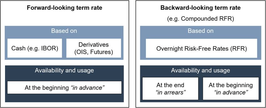
The Figure shows the typical design of a variable-rate cash product. By using a term rate that is pre-determined such as
LIBOR, the next interest payment is known at the beginning of each interest period. By contrast, all RFRs are overnight rates.
There are two ways of constructing term reference rates based on realisations of RFRs. One method, known as compounding
‘in arrears’, relies on the realisation of overnight rates over the same period as the interest rate period, and hence is only known
at the end of the period. The second method, known as compounding ‘in advance’, relies on compounded realisations of RFRs
over the same horizon as the interest rate period, but lagged by one interest rate period so as to arrive at a pre-determined
reference rate.
compounded rate, as expectations can shift quickly.5 What is more, having a liquid underlying market
is a core requirement for benchmarks, as noted in the FSB (2014) and IOSCO (2013) publications.6 While
there has been a strong push in recent years to develop derivatives markets based on RFRs such as SOFR
in the US and these markets have indeed grown over the past years, liquidity in RFR-linked derivatives
is still not sufficient to support robust benchmarks. Another downside is that liquidity in derivatives
markets can quickly evaporate during crises. The main problem of LIBOR is the lack of the underlying
activity supporting the benchmark rate. To avoid repeating the same mistake, it is preferable that
products reference robust and reliable benchmarks, i.e. the RFRs themselves and not the RFR-based
derivative markets.
RFRs can be used to construct term rates by compounding the (overnight) RFRs over the relevant
period. By doing so, this term rate is known at the end of an interest period, which is typically referred
to as compounded RFR ‘in arrears’. One could argue that in the ideal post-LIBOR world, all products
should use a compounded RFR ‘in arrears’ as a term rate. In fact, some derivatives markets have been
5 In Switzerland, the above arguments were the main reasons why a forward-looking rate based on derivatives was not
recommended by the national working group, as stated in the minutes of October 2018.
6 In the UK and EU, the usage of a benchmark in contracts can be prohibited in case the underlying market becomes illiquid
and the relevant regulator declares the benchmark non-representative. See EU Benchmark Regulation.
2able to function well based on this approach for quite some time. Using compounded O/N interest rates
‘in arrears’ is standard to settle the payment obligations in Overnight Indexed Swaps (OIS).7 Ideally, a
compounded RFR ‘in arrears’ would be used for both derivatives and for variable rate cash products.
This in turn would allow to perfectly hedge cash products and to price fixed rate products, e.g. based
on OIS. Therefore, it would be ideal to also use a compounded RFR in cash products.8 Indeed, over
the past two years several floating rate notes (FRNs) based on SOFR and SONIA have been issued.9
However, adoption of compounded RFRs ‘in arrears’ in the loan market (with the exception of SARON
in Switzerland) has been sluggish so far. Various factors—some of them related to how market plumb-
ing is set up—make a transition to an ‘in arrears’ approach difficult for certain groups of cash market
participants. For this reason, many market participants have adopted a “wait and see” approach until
the existence of a forward-looking term rate. A cash market waiting for a forward-looking term rate
leads to a chicken-and-egg problem, in the sense that it is hard for the derivatives market to become
liquid in absence of a deep cash market (and vice versa). Yet, for many cash market applications, it is
not so much the forward-looking element that is necessary, but rather the fact of being able to know the
rate ahead of the interest rate period, i.e. to have a pre-determined rate.
In this note, we propose to solve this chicken-and-egg problem by using past RFRs known at the
beginning of an interest rate period in order to define a pre-determined term rate. One can think
of the approach—sometimes also referred to as a compounded RFR ‘in advance’—as a lagged ver-
sion of the ‘in arrears’ approach. Just like LIBOR, the ‘in advance’ approach offers the benefit of pre-
determinedness that certain participants in cash markets require. To be sure, this approach however
does not replicate the forward-looking nature of LIBOR, nor does it contain a credit and liquidity-
sensitive component that fluctuates with banks’ marginal funding costs (see Schrimpf and Sushko
(2019), Syrstad and Klingler (2019), Berndt, Duffie and Zhu (2020), and Bowman, Chiara and Vojtech
(2020) for recent discussions).10 However, an important implication of our findings is that for a range of
applications it is rather the pre-determinedness that matters and not so much the feature that the term
7 OIS are the most common derivative product based on overnight rates. An OIS is an interest rate swap in which it is
agreed to exchange a payment based on the difference between the fixed rate and the compounded overnight rate. The
payments occur at the end of each interest period until the OIS contract reaches its maturity. The OIS rate is the fixed leg of
such a swap, and reflects the expected path of the overnight rate over the contract term.
8 See also the work done by the National Working Group on Swiss Franc Reference Rates (NWG), which recommends using
a compounded SARON, the Swiss RFR, wherever possible. See NWG (2018).
9 See also a Table published by LMA, which lists out RFR referencing loans or a Table published by ICMA on RFR based
FRNs. Furthermore, several banks started to launch SARON-based mortgages.
10 While a deeper analysis is outside of the scope of this note, a credit and liquidity-sensitive component could be beneficial
for financial market participants to trade and hedge risks related to the evolution of funding market conditions. It is conceiv-
able that the term RFRs we advocate could in principle also be combined with other approaches capturing credit-sensitivity.
In this context, see Berndt et al. (2020) who propose a methodology for constructing a credit-sensitive complement to SOFR.
3rate is forward-looking. An approach based on past RFRs alone (even if lagged) can work reasonably
well in many cash market applications, and we provide some practical guidance that can help market
participants with the use of such RFR term reference rates. It could also serve as a useful option in
currency areas with less developed derivatives markets, in particular emerging market economies.
The main counter-argument against the ‘in advance’ methodology is that the rate, while being pre-
determined, will be sluggish to respond when interest rate expectations change. By construction, a
backward-looking rate will not be as responsive as say a forward-looking term rate based on RFR-
derivatives would be. The lagged behavior of a compounded RFR ‘in advance’ may at times create a
mismatch to a compounded RFR ‘in arrears’. This ‘basis’ is simply the difference between two consecu-
tive compounded rate and can be especially pronounced when the central bank adjusts its policy rates
during an easing or tightening cycle.11
This note analyses two main ways how market participants can manage the basis that stems from
using an “in advance” term rate in cash products. As a first step, we derive what we call the ‘advance’
basis and illustrate under what conditions it arises. We then show that the basis by using an ‘in advance’
rate can be priced. The estimated basis at the start of the financial contract in turn can be used as an
adjustment factor to match the present value of an “ideal” contract using an RFR compounded ‘in
arrears’. One can also think of this adjustment factor as a convenience premium to have the reference
rate pre-determined. Furthermore, we show that this adjustment factor can be hedged by either using
existing derivatives, such as an OIS, or through contractual features. The second option to reduce the
basis is to rely on shorter observation periods prior to the interest period when calculating the pre-
determined term rate. In this way, the term rate becomes more responsive, as not the entire past period
is used for the calculation. Our empirical analysis suggests that using a shortened observation period
is indeed a sensible way to reduce the basis from using an “in advance” term rate. For instance, using
the RFRs compounded over the week prior to the interest period to determine the interest payments for
the next three months, leads to a basis which is low on average and also not too volatile. At the same
time, the approach still allows for payments to be on a quarterly basis.
To investigate the various approaches, we rely on empirical data for the effective federal funds rate
(EFFR), which is also an O/N rate like the identified RFRs. While EFFR is not the chosen RFR in the US,
we use it in our examples due to the longer history than the secured overnight funding rate (SOFR).12
11 Note that for reasons that become clearer below, usage of a forward-looking term rate based on derivatives, will also
entail a basis that can be substantial at times.
12 LIBOR is fixed in five currencies and therefore the same analyses could be done for the other RFRs chosen by the author-
ities in these jurisdictions. However, the key messages would remain unchanged.
4This is especially important when we compare backward-looking RFR term rates to forward-looking
term rates based on derivatives (there is only a short history of OIS linked to SOFR, but there is a long
history and deep OIS market linked to EFFR).
Our findings have several key practical implications. The approaches analyzed here could help
foster the usage of a compounded RFR ‘in advance’ in case a pre-determined rate is needed. Hence,
they may be especially relevant for smaller market participants in cash markets, that otherwise could
occur high switching costs in their back-office operations towards an ‘in arrears’ reference rate. As
the ‘in advance’ term rate already exists and is underpinned by the robust RFRs, usage of the rate in
cash contracts may help to accelerate the transition away from IBOR-style benchmarks. The approach
we focus on in this note ensures a robust anchor for term rates, as the construction is solely based on
the RFRs themselves that are underpinned by strong market activity and trading volume.13 Deter-
mining the ideal methodology for pre-determined interest payments, will play an important role in a
post-LIBOR world. Experience with the current reform and similar past episodes suggests that once a
tipping point has been reached (McCauley, 2001) and a benchmark is widely used, it is challenging to
transition away from it. It is therefore important to identify the ideal methodology for benchmark rate
construction from the start, i.e. before it is actually used.
The remainder of this note is structured as follow. Section 2describes the current preferences for a
pre-determined term rate. Section 3 investigates the behavior of compounded backward-looking terms
rates and the basis that results from using forward-looking rates based on derivatives and compounded
rates ‘in advance’. Section 4 discusses several practical ways to reduce the ‘in advance’ basis. Section 5
provides a summary of the properties of various term reference rate approaches. Section 6 concludes.
2 Why do some end-users prefer a pre-determined term rate?
Consultations with end-users of financial benchmarks in various currency areas indicate that there
are some important groups of users, notably small to medium-sized corporates and retail clients that
have expressed a preference for pre-determined term reference rates. Financial institutions and large
corporates, by contrast, have indicated that a pre-determined rate is for most products not required,
13 In the FSB (2014) and IOSCO (2013) publications it is stated that a benchmark should be based on a robust underlying
basis, i.e. is based on a liquid market segment where ideally the calculation of the benchmark is based on actual transactions.
This is questionable in the case of LIBOR (see, e.g. Bailey, 2017). The newly identified RFRs, however, are all robust, which was
one of the main criteria why they were recommended as successor rates to LIBOR. A robust underlying basis, in combination
with a strong governance structure, minimises the risk for manipulation and allows for a credible benchmark.
5with some partially already starting to use RFRs compounded ‘in arrears’.14 The working group in the
UK states that, while ideally a RFR compounded ‘in arrears’ should be used as a term rate, about 10%
of the total loan volume is currently not feasible with an ‘in arrears’ structure.15 The number of loans
for which an ‘in arrears’ structure is not workable is likely to be higher as most loans relate to smaller
and less sophisticated borrowers.
It is worth to have a closer look at why certain clients express a preference for a pre-determined term
rate. As discussed above, for most of these market participants it is not so much the forward-looking
component that LIBOR used to provide that matters, but rather the pre-determinedness of the interest
rate. To these market participants, cash flow certainty has the following advantages:
Cash flow management: Smaller market participants do not have a sophisticated treasury team and
therefore would need to increase their liquidity holdings to mitigate the increased cash flow uncer-
tainty. This would result in higher costs for those market participants. By having an account at the
lending institution these costs can be reduced, but still additional liquidity would need to be held at
this account. For sophisticated market participants, this argument is less relevant, as they could in
principle hedge cash flow uncertainty via derivatives such as an OIS.16
IT-systems: Most IT systems that are currently in use require cash-flow certainty. In a standard
‘in arrears’ structure, the final interest rate is known on the last day of an interest period. There are
modified ‘in arrears’ structures which allow for a few additional days, but even these options are not
compatible with legacy systems. LIBOR became widely used at a time when IT-systems required mostly
manual input. So far, most systems are not yet capable of handling a rate that is only known at the end
of an interest rate period.17 This issue can be solved in the long run, but it might not be possible for some
system providers to do so before the cessation of LIBOR. It could also be an issue for market participants
in currency areas other than the LIBOR currencies, where system providers feel less pressure to adapt.
Current hedging instruments: LIBOR has been a cornerstone of financial markets for decades, and
many hedging instruments and market conventions have evolved around it. For example, market par-
ticipants with assets and/or liabilities in several currencies use FX swaps and/or cross currency basis
swaps (CCBS) to concentrate cash flow management in a single currency. These instruments are based
on knowing the rate at the beginning. To solve this issue, existing instruments can be combined with an
14 See e.g. FSB interim report 2019.
15 See Use Cases of Benchmark Rates by UK WG above.
16 A fixed-rate receiver OIS at the beginning of each interest period could be conducted to achieve cash flow certainty.
17 Infrastructure providers in Switzerland have updated their systems to include also the possibility of a term reference rate
compounded ‘in arrears’.
6OIS contract. Also, new instruments, e.g. RFR-based CCBS are being developed. That said, experience
tells that market development for such new instruments is not a rapid process as new conventions need
to be established and that it takes time until these markets are liquid.
Legal restrictions: In some jurisdictions, retail loans require a longer notification period. In the US
for instance, consumer regulations define a minimum notification period of 45 days for retail loans. EU
consumer regulation does not itself define such a minimum notification period, but the text leaves this
possibility open for member states.18 Those regulations were written before RFRs were recommended
as successor rates to LIBOR. However, an amendment is unlikely. Furthermore, an ‘in arrears’ structure
is not compatible with Islamic finance, which requires a pre-determined interest rate.
Tough legacies: Additionally to new contracts which can be designed to use RFRs, there are outstand-
ing LIBOR-based contracts with a maturity beyond 2021. Of those outstanding LIBOR contracts there
are some contracts which cannot be transitioned to a compounded ‘in arrears’ RFR, e.g. due to technical
or legal reasons. Currently there are new regulations proposed and discussed, which can solve legal
issues. Nevertheless, a pre-determined rate might still be required in order to solve technical issues.19
To sum up, due to the aforementioned reasons some groups of market participants express a pref-
erence for a rate known at the beginning of the interest rate period, as opposed to a term rate based on
compounding ‘in arrears’. However, for all above reasons the rate only needs to be pre-determined—
it does not need to contain a forward-looking element by reflecting market expectations.20 Hence, a
‘backward-looking rate in advance’ can serve as a viable alternative rate to an in-arrears RFR in those
circumstances.
3 Characteristics of alternative term rates
In this section, we illustrate the characteristics of various types of term references rates. To this end, we
compare them with the ideal case of an ‘in arrears’ RFR term rate. We thus explicitly calculate the basis
from using either a backward-looking ‘in advance’ rate or a forward-looking rate based on derivatives,
as the difference with respect to the ‘in arrears’ rate (which serves as reference for these comparisons).
As an illustration, we first start by looking at the Secured Overnight Financing Rate (SOFR), which
18 In
German law there does not seem to be such a requirement.
19 See
the proposed legislation by the UK Government.
20 The only exception are products, where the notional can change after or during each interest period, e.g. trade finance.
Products with a variable notional should ideally use an RFR compounded ‘in arrears’ or contractual agreements for a delayed
compensation in case an RFR compounded ‘in advance’ is used. However, in most products the notional remains constant
until maturity.
7is the recommended alternative for U.S. dollar (USD) LIBOR.21 Figure 2 depicts the development of
SOFR since 2002 (light blue line). As the first publication of SOFR was only on August 4, 2018, we
used proxies for SOFR provided by Bowman (2019) that stretch back a longer period. The compounded
SOFR ‘in arrears’ for the last 90 calendar dates is shown with the dark blue line in the graph.22 The
compounded rates lag SOFR, as they are depicted at the end of each 3-months period (in line with the
‘in arrears’ structure).
Figure 2: SOFR and compounded SOFR (90 days)
in
% percent
5.00
4.00
3.00
2.00
1.00
0.00
2002 2004 2006 2008 2010 2012 2014 2016 2018 2020
SOFR 3M SOFR in arrears
Sources: Bloomberg, Bowman (2019), authors calculations
The Figure shows the overnight rate SOFR and the 3-months compounded SOFR rate ‘in arrears’.
The first important point to note by looking at Figure 2 is that the compounded SOFR is far less
volatile than SOFR itself. Even the spike, which occurred in September 2019, did not have a significant
effect on compounded SOFR.23 Especially for smaller and less sophisticated market participants it is
beneficial to have a term reference rate that is not too volatile in order to facilitate their cash flow
management.
The compounded RFR ‘in arrears’ can be considered as an ideal case against which various pre-
determined term rates can be compared. In the following, we will hence look at the ‘basis’, computed
as the difference between various pre-determined term rates and the ‘in arrears’ rate C3m,i which serves
as the reference for these comparisons:
21 See the webpage of the Alternative Reference Rates Committee (ARRC) for further information. The ARRC is a group
of private-market participants convened by the Federal Reserve Board and the New York Fed to help ensure a successful
transition from USD LIBOR to a more robust reference rate, its recommended alternative, the SOFR.
22 The formula how to calculate the compounded SOFR can be found in the Appendix.
23 Figure A.2 in the appendix compares day to day volatility of different rates and shows that forward-looking rates are far
more volatile than a compounded rate (see also user guide on SOFR).
8α3m,i = OIS3m,i − C3m,i (1)
β 3m,i = C3m,(i−1) − C3m,i . (2)
The forward basis α captures the mismatch of using a forward-looking term rate based on derivatives
(here OIS) and the compounded SOFR in arrears. In a similar vein, the advance basis β is computed as
the difference in the compounded SOFR in advance and the compounded SOFR in arrears. i refers to
the first day of the period. Hence, β 3m,i is the difference of the compounded rate over the last lagged
3-months period up to date i (‘in advance’ rate) minus the compounded rate over the next 3-months
period (‘in arrears’ rate). This means that β 3m,i is only known at i + 3m, that is, after the path of SOFR
is known to allow for the computation of the ‘in arrears’ rate.
Figure 3: Basis of pre-determined term rates: illustration for EFFR
in percentage points
PP %
in percent
2.00 6.00
5.00
1.00 4.00
3.00
0.00 2.00
1.00
-1.00 0.00
2002 2004 2006 2008 2010 2012 2014 2016 2018 2020
alpha beta EFFR (rhs) 3M EFFR in arrears (rhs)
Sources: Bloomberg, authors calculations
The Figure shows the overnight rate EFFR and the 3-months compounded EFFR rate ‘in arrears’. The forward basis α is the
difference between the fixed rate of OIS linked to EFFR and the compounded EFFR ‘in arrears’. The maturity of both rates
is three months (3m). The advance basis β is the difference between the in 3-months advance compounded EFFR minus the
3-months compounded ‘in arrears’ EFFR.
Figure 3 depicts the behavior of various types of term rates, using EFFR for illustration. EFFR and
OIS rates where EFFR is the underlying O/N rate have already a history of 20 years and (unlike SOFR)
do not require the usage of proxies. While EFFR is not the chosen RFR in the US, the main insights
derived from the analysis of EFFR will also carry over for SOFR or other RFRs. The graph shows both
the daily O/N rate and the 3-months compounded term rate ‘in arrears’. In addition, the graph shows
the two basis measures for the 3-months compounded ‘in advance’ EFFR and a forward-looking rate
(α3m,i ). For the latter, we rely on the 3-months OIS rate which is linked to EFFR.
9As expected, both bases are close to zero during times of constant interest rates. In case of abrupt
unexpected interest rate changes, e.g. around the great financial crisis in 2008, there is a large increase
in both basis measures. The main reason is that neither the ‘in advance’ term rate nor the OIS rate
capture the extent the Fed cut policy rates in this period.24 The graph also shows that the forward basis
between 2010 and 2016—the period when short-term interest rates were close to their effective lower
bound—is close to zero. This suggests that excess returns in the OIS market have been close to zero in
this period.25
In contrast to the forward basis (which can be affected by term premiums embedded in the pricing
of money market derivatives, at least conceptually), the advance basis should on average be zero when
looking over a longer-run interest rate cycle. However, for a single interest period the advance basis can
be substantial. Figure 4 illustrates the link between the length of the contract period and the average
advance basis. It depicts the advance basis for each 3-months interest period (β 3m,i ) and how on average
the advance basis decreases with increasing length of contracts. The average advance basis by using 3-
months interest periods over the next two years starting at i is denoted as β 3m,2Y . For five-year contracts
e.g. starting 2010, the average advance basis (β 3m,5Y ) was zero, as interest rate remained constant until
2015.
Figure 4: Average advance basis depending on contract length
in percentage points
PP
2.00
1.50
1.00
0.50
0.00
-0.50
-1.00
2002 2004 2006 2008 2010 2012 2014 2016 2018 2020
beta i EFFR 1Y beta 2Y beta EFFR 5Y beta
Source: Bloomberg, authors calculations
The Figure shows the advance basis of EFFR for 3-months interest periods (β 3m,i ) and the average advance basis for certain
contract lengths, e.g. the average advance basis for 3-months interest periods over the next two years ( β 3m,2Y ). The average
basis is shown at the beginning of the period of each contract.
24 For an in depth analysis of monetary policy expectation errors and excess returns in money market derivatives, see
Schmeling, Schrimpf and Steffensen (2020).
25 Excess returns in derivatives occur either due to wrong expectations or due to term premium component embedded in
the derivatives pricing. See e.g. Longstaff (2000), Schmeling et al. (2020) or Fuhrer, Guggenheim and Juttner (2019).
104 Minimizing the advance basis
This section analyzes two different approaches of minimizing the advance basis that arises when using
a compounded RFR ‘in advance’. The first approach is to use a constant adjustment factor in order
to compensate for the advance basis. The adjustment factor in turn can be determined based on the
pricing in the OIS market. The second approach is to use a shorter observation period (say only one week)
to reduce the advance basis while interest periods are still three months.26
4.1 How to price and hedge a pre-determined adjustment factor
In order to price an ‘in advance’ product, one can compare its present value with that of an ‘in arrears’
product. Consider first an example, where for simplicity we do not discount the future cash flows.
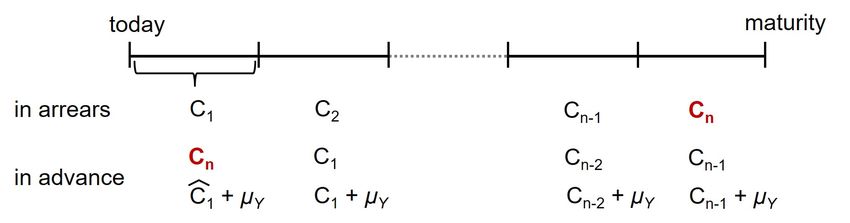
Figure 5 illustrates a cash product with n interest rate periods, where Ci is the compounded ‘in arrears’
rate of period i. Hence, Ci is always only known at the end of each period i. In the ‘in advance’ product,
each compounded rate is by definition lagged by one period. But, even though the interest payments
are delayed by one period, they are not lost. Only the compounded rate of the last period (Cn ) is lost
by using an ‘in advance’ structure. Hence, the difference in the present value of the two products is
primarily driven by the last compounded interest rate (Cn ).
Figure 5: Pricing the adjustment factor (µY )
The Figure illustrates a simplified stream of interest rate payments (Ci ) for an ‘in arrears’ product. If the ‘in advance’ product
uses Cn for the first cash flow, both products have roughly the same present value. Cn has to be estimated ex ante and can
be split over the various interest periods (µY ). As µY is a fixed number agreed at the beginning of the contract, requirements
regarding the underlying data basis are less stringent.
To achieve the same present value, the simplest approach would just be to use an estimate of the
last cash flow C
cn as the first rate of the ‘in advance’ structure. The first rate does not have to fulfil
26 All options described in this note define the interest payment at the beginning of a period. There are even further options
to achieve a pre-determined interest rate as described in the guide for overnight rates, such as the option ‘interest rollover’. In
these additional options, past interest payments influence the next interest payment. While this feature conflicts with current
standards, it shows that there are many ways to avoid using a forward-looking rate and still have a pre-determined interest
rate.
11the requirements of a benchmark rate to be robust, as it could be bilaterally agreed on between the
two counterparties at the start of the contract. Alternatively, one can also agree on using an estimation
of C1 at the start of the contract (C
c1 ) and add to each compounded rate a constant adjustment factor
(µY ), where Y denotes the duration of the contract in years. By including this adjustment factor, the ‘in
advance’ product achieves the same present value as the ‘in arrears’ product. As µY is constant and is
bilaterally agreed on at the start of the contract, it does not need to be based on a robust underlying
market as would be the case for interest rate benchmarks.
The following simple formula can be used to price µY (see the Appendix C for the derivation):
cn − C
C c1
µY = . (3)
n
The adjustment factor depends on the difference in interest rates between the beginning and the
end of the contract as well as on the number of periods n during the life of the contract. Hence, the
adjustment factor decreases with shorter interest periods, and it decreases with the duration of the
contract for unchanged period lengths, as both increases n. In case of identical interest rates at the
beginning and the end of the contract, the adjustment factor is zero, independent from the duration of
the contract, the lengths of interest rate periods or the interest rate path.
Ex post, the adjustment factor is known, as it is the difference between the present value of an
‘in arrears’ and an ‘in advance’ product, i.e. the average advance basis over the life of the contract.
However, this is not known ex ante. In order to estimate the adjustment factor, the formula below can
be used. The main input into the formula is an estimate of the last period’s expected cash flow C
cn .
To this end, the OIS rate with a similar maturity (Y) as the cash contract can be used, as shown in the
equations below.27
Cn − C1 Cn + C1
OISY ≈ + C1 = (4)
2 2
Cn = 2OISy − C1 (5)
cn − C
C c1
µY = (6)
n
2(OISy − C
c1 )
µY ≈ (7)
n
27 The OIS rate reflects the expectation of the average underlying O/N rate over the maturity of the OIS contract. Instead
of the OIS rate, one can also use a forward starting in Y years, which reflects the expected average of the underlying rate only
over the last interest period, i.e. C
cn . This would result in a better estimation, as it does not depend on the expected interest
rate path until the last period. However, forwards may not be available for longer maturities.
12The above equation for the adjustment factor can be used as a simple rule of thumb to price the
expected advance basis over the life of the contract. By applying the adjustment factor, the expected
present value of the ‘in advance’ structure matches that of the ‘in arrears’ structure.
The following equation gives the advance basis with adjustment factor:
γ3m,2Y = C3m,(i−1) + µY − C3m,i . (8)
How well the estimation for the advance basis matches the realised advance basis ex post, crucially
depends on the quality of interest rate expectations. As an example, in 2004, before the Federal Reserve
under Chairman Greenspan started its hiking cycle, the OIS rate for a two-year contract was around
3%, while the EFFR was around 1%. With two years and quarterly interest periods, n equals 8. By
using the equation above, this results in an estimated advance basis (c
β y ) of 0.50% over the life of the
contract. This number, known at the beginning, matches quite well the average daily β 3m,i based on
the realizations over the next two years. Hence, by using the estimated advance basis as a adjustment
factor, the advance product would have roughly the same return as the ‘in arrears’ product.
Interest rate expectations can of course also be wrong. Figure 6 shows the advance basis in case no
adjustment factor, together with the basis where an adjustment factor is applied (β 2Y + µ2Y ). The basis
by applying an adjustment factor was fairly low around 2004, as interest rate expectations correctly
reflected the future interest rate path. There may be periods, however, where this is not the case due to
substantial expectation errors regarding the course of monetary policy (Schmeling et al., 2020).
There are two ways to hedge against unexpected interest rate developments. The first way is to
hedge using derivatives. As µY is priced by using OIS, it can also be hedged with an OIS. The notional
of the OIS should be equal to the n-th fraction of the loan volume. The second way is to contractually
hedge µY by agreeing to exchange with the last interest payment the difference compared to an ‘in
arrears’ structure. To avoid outstanding payments after the maturity of the loan and to continue using
a pre-determined interest rate, the difference could also be calculated at the beginning of the last interest
period and paid at maturity. The minor interest rate risk of the last period would thereby be neglected.
Such a contractually agreed hedge would even offset differences due to the approximation used to
calculate µY . The same approach could be chosen to handle early redemption. The disadvantage of the
second approach would be the added contractual complexity.
13Figure 6: Basis for two-year contracts with and without adjustment factor (µY )
PP
in percentage points
1.50
1.00
0.50
0.00
-0.50
-1.00
2002 2004 2006 2008 2010 2012 2014 2016 2018 2020
2Y beta error after mark-up + μ2Y
Source: Bloomberg, authors calculations
4.2 Shortened observation period with unchanged interest periods
Another approach to reduce the advance basis is to use a shortened observation period in the calcu-
lation of the pre-determined backward-looking rate. In our analysis below, we use the compounded
EFFR during a one-week observation period before each interest period started C1w,(i−1) . The resulting
basis with respect to the in arrears rate is then given as:
δ3m,2Y = C1w,(i−1) − C3m,i . (9)
Figure 7 shows the basis δ3m,2Y that occurs when only observations from one week (instead of three
months) are used for the construction of the in advance term rate. As before, we calculate the discrep-
ancy with the ‘in arrears’ rate for two-year contracts with three-month interest periods. The Figure
shows that using a shortened observation period (δ3m,2Y ) performs far better than using the standard
‘in advance’ rate (β 3m,2Y ). It also performs significantly better than the approach of using an adjustment
factor (γ3m,2Y = β 3m,2Y + µY ).
The key underlying reason is that with a shortened observation period the term rate becomes far
more responsive to changing market conditions, which in turn can mitigate discrepancies from the ex
post ‘in arrears’ rate. A downside of the approach of using shortened observation periods is the greater
volatility of the resulting term rate, as the shortened observation period implies less smoothing. In the
14case of EFFR, the volatility by using one week observation periods, however, turns out to be roughly
similar as that when using three-month forward-looking rates such as LIBOR or OIS (see Figure A.2
in the Appendix). Also note that the basis from using this rate cannot be hedged by using existing
derivatives but by contractually agreeing to exchange differences with the last interest rate payment.
This option to construct term rates is quite promising because it is easy to implement, generates a small
basis vis-a-vis the ideal in arrears rate, while still allowing for three-month interest periods.
5 Summary of approaches to reduce the basis
This note starts from the premise that in the post-LIBOR world, it would be most sensible if all contracts
rely upon a compounded RFR ‘in arrears’ term rate. Derivatives markets have been relying on this
structure for a long time. If also cash markets use a compounded RFR ‘in arrears’, it would allow to
perfectly hedge cash products and to price fixed rate products, e.g. based on OIS. Furthermore, such a
term rate is already available, as it only requires the RFR itself.
The devil is in the details, though. Not all cash products can handle a compounded RFR ‘in arrears’
and there is a host of other institutional obstacles and switching costs (see discussion in Section 2). We
therefore investigate various bases comparing the discrepancies between different pre-determined term
rates and the in arrears rate which is only known ex post.
Figure 7 provides an illustration of all the approaches compared in this note, again by looking at
the basis with respect to the in arrears reference case. In the comparison, we use two-year averages, i.e.
show the average basis for two-year contracts at the beginning of the contracts.
The first basis we look at is the forward basis(α3m,2Y ), here computed based on OIS rates as a proxy
for the forward-looking term rate. However, such term rates do not yet exist, and it is questionable if
there is a robust underlying market to support such a rate as a benchmark. We thus consider different
types of ‘in advance’ term rates, which are also pre-determined. The basis when using the standard
version of an ‘in advance’ term rate is denoted by β 3m,2Y . This basis is the difference between two
consecutive compounded rates and can be especially pronounced when the central bank adjusts its
policy rates during an easing or tightening cycle (as discussed above). The third approach (γ3m,2Y )
uses a constant adjustment factor during the contract period (2Y) in order to minimize the basis. The
adjustment factor can be viewed as a convenience premium to have the interest rate pre-determined.
We show that the adjustment factor can be priced, e.g. by drawing on expectations derived from the OIS
curve. However, as expectations do not necessarily match realizations, an adjustment factor estimated
15Figure 7: Minimizing the advance basis: an overview of different approaches
in percentage points
PP
1.40
1.20
1.00
0.80
0.60
0.40
0.20
0.00
-0.20
-0.40
-0.60
2002 2004 2006 2008 2010 2012 2014 2016 2018 2020
2Y alpha 2Y beta bias with m gamma2Y 2Y delta
Source: Bloomberg, authors calculations
The Figure shows the various bases by using contracts with a two-year term. All bases are shown at the beginning of the
respective contracts. The relevant bases are computed for three-months interest periods. For comparison purposes, also a
basis β 1m,2Y is with one month interest periods (dashed line).
upfront based on expectations can lead to a rather elevated and volatile basis (γ3m,2Y ). The fourth
approach is an in advance rate that uses a shortened observation period δ3m,2Y .
Table 1 below gives a summary of the properties of the various basis, in particular how large they
are on average (mean) and how volatile they are (standard deviation). The Table shows that the mean of
the forward basis (α3m,2Y ) is larger than that of the advance basis (β 3m,2Y ), as interest rate expectations
embedded in money market derivatives do not always capture sharp policy rate cuts by the central
bank. While the mean for the advance basis should be zero in the long-run, it turns out to be slightly
positive in our sample as the interest rate level was around 150 basis points higher in 2002 than in
2020.28 The standard deviation of the advance basis (β 3m,2Y ) also tends to be higher than that of the
forward basis (α3m,2Y ), as interest rate cuts and hikes always lead to an advance basis. However, in case
of day-to-day changes, a compounded rate based on past rates is far more stable than a forward looking
rate, as shown in Figure A.2.
Table 1: Evaluation of the basis between 2002 and 2020 (in basis points)
α3m,2Y β 3m,2Y γ3m,2Y δ3m,2Y β 1m,2Y
mean 4 2 21 0 1
standard deviation 15 36 37 20 15
28 The long-run mean for the advance basis can be calculated by using Equation 3. With an interest rate change of 150 basis
points, quarterly periods and 18 years (70 interest periods), the advance basis or ideal but ex-ante unknown adjustment factor
is two basis points.
16Looking at the performance of the two variants of in advance rates to mitigate the basis, we find
clear support for the approach that relies on shortened observation periods (1-week in our example).
The mean of the δ3m,2Y basis is the smallest among of the options analysed, and its standard deviation is
also only slightly higher than that of α3m,2Y . By contrast, the mean of the basis when using an adjustment
factor is elevated (γ3m,2Y ). This could owe to the fact that the adjustment factor needs to be based on
expectations over two years, which frequently do not match realizations. For a similar reason, the
standard deviation γ3m,2Y is rather large. All in all, these findings indicate that the approach based
on shortened observation periods emerges as a promising and quite robust methodology for term rate
construction when a pre-determined rate is needed.
6 Conclusion
In LIBOR-based products the term reference rate is known at the beginning of each interest period. By
contrast, with the transition to overnight risk free rates (RFR), the term reference rate is usually known
at the end of an interest period (‘in arrears’). This approach is already the standard for derivatives based
on overnight rates. For cash products, though, many market participants indicate a preference to know
the rate before the start of the interest rate period. This presents an obstacle to the adoption of RFRs for
cash products and also leads to subdued demand for RFR-based derivatives. The preference for pre-
determined term rates is driven by a range of factors (e.g. IT-systems currently being unable to handle
term rates based on ‘in arrears’ compounding, a simplified liquidity management, misalignment with
current hedging instruments, e.g. FX swaps, and regulations requiring a longer notification period for
retail loans). Some of these road-blocks can be overcome in the longer-run, but not necessarily before
the envisaged phase-out of LIBOR.
A forward-looking term rate based on RFR-derivatives appears to be the solution. But, such a
rate depends not on the robust RFR itself but on the derivatives-markets for RFR. Most RFR-based
derivatives-markets are not yet liquid and can quickly become illiquid in crises. The core problem of
LIBOR is the lack of activity in the underlying market LIBOR is based on. To avoid similar issues, cash
products should ideally reference the RFRs that are underpinned by an active market, as opposed to
yet another rate constructed from a derivatives market with questionable underlying liquidity.
Another, and much simpler, solution is to use past RFRs to define the term reference rate at the
beginning of an interest rate period (backward-looking ‘in advance’). So far, this solution has not been
widely discussed as critics have pointed to the issues arising from its lagged behaviour in periods when
17policy rate change. A key message of this note is that the resulting basis from using an ‘in advance’ rate
can be managed, thereby rendering the rate an attractive option for certain market participants and
currency areas without developed interest rate derivatives markets.
Adapting backward-looking ‘in advance’ term RFRs for those cash products where an ‘in arrears’
rate is currently not feasible, may help smoothen the transition away from LIBOR. The use of bench-
marks in financial contracts leads to a strong path dependency, since a transition is very costly in ret-
rospect. RFRs such as SOFR are very robust, already available and based on highly liquid underlying
markets. Market participant are currently at crossroads and have to choose how to replace LIBOR in
financial contracts. Against this backdrop, this note may offer some practical guidance of how simple
‘in advance’ term reference rates can be used in case a pre-determined rate is needed.
This note evaluates two practical ways of how market participants can reduce the basis from using
an ‘in advance’ term rate based on RFRs. One approach is to use the RFRs of the last period as a term
rate and to add an adjustment factor to compensate the basis. The second approach to reduce the basis is
to rely on shorter observation periods prior to the interest period when computing the pre-determined
term rate. This term rate is more responsive to changing market conditions, as fewer past observations
are used for the calculation.
We conclude based on our analysis that the most promising option to reduce the basis from using
an “in advance” term rate is in fact to use a shortened observation period. By using the overnight RFRs
compounded over the week prior to the interest period to determine the interest payments for the next
three months, the basis will be relatively minor and not very volatile, while payments are still on a
quarterly basis.
18References
Bailey, Andrew (2017) “The future of LIBOR”, Speech by Andrew Bailey, Chief Executive of the FCA.
Berndt, Antje, Darrell Duffie & Yichao Zhu (2020) “Across-the-Curve Credit Spread Indices”,
manuscript.
Bowman, David (2019) “Historical Proxies for the Secured Overnight Financing Rate”, FEDS Notes.
Washington: Board of Governors of the Federal Reserve System.
Bowman, David, Scotti Chiara & Cindy Vojtech (2020) “How Correlated is LIBOR with Bank Funding
Costs?”, FEDS Notes. Washington: Board of Governors of the Federal Reserve System.
Duffie, Darrell & Jeremy Stein (2015) “Reforming LIBOR and Other Financial Market Benchmarks”,
Journal of Economic Perspectives, 29, pp. 191–212.
FSB (2014) “Reforming Major Interest Rate Benchmarks”, FSB Publication.
Fuhrer, Lucas, Basil Guggenheim & Matthias Juttner (2019) “A survey-based estimation of the Swiss
franc forward term premium”, Swiss Journal of Economics and Statistics.
IOSCO (2013) “Principles for Financial Benchmarks”, IOSCO Publication.
Longstaff, Francis A (2000) “The term structure of very short-term rates: new evidence for the expec-
tations hypothesis”, Journal of Financial Economics, 58 (3), pp. 397–415.
McCauley, Robert N (2001) “Benchmark tipping in the money and bond markets”, BIS Quarterly Re-
view.
NWG (2018) “Minutes from the 20th meeting of the National Working Group on Swiss Franc Reference
Rates”, Minutes.
Schmeling, Maik, Andreas Schrimpf & Sigurd Steffensen (2020) “Monetary Policy Expectation Er-
rors”, Available at SSRN.
Schrimpf, Andreas & Vladyslav Sushko (2019) “Beyond LIBOR: a primer on the new benchmark
rates”, BIS Quarterly Review.
Syrstad, Olav & Sven Klingler (2019) “Burying Libor”, Norges Bank, Working Paper 13/2019.
19A Terminology of term rates
Figure A.1: Terminology of term rates
See also user guide for overnight risk-free rates published by the FSB.
20B Formula for compounding of O/N rates
" #
db
rj nj
360
Ci = ∏ 1+
360
−1
dc
(A.1)
j =1
The compounded RFR for period i (Ci ) can be calculated by using the above formula, where j repre-
sents a series of numbers representing each business day in the period, db the total number of business
days in the period, dc the total number of calender days in the period, n j the number of calendar days
for which rate r j applies, and r j is RFR on business day j of the period.
21C Derivation of the adjustment factor to compensate for the in-advance
basis
The present value of an ‘in arrears’ product (PVarr ) and of an ‘in advance’ product (PVadv ) can be used
to derive the adjustment factor (µY ) used to compensate for the advance basis. The compounded rate of
period i is denoted by Ci , n denotes the overall number of interest periods and m denotes the number
of interest periods per year.
n
Ci
PVarr = ∏ 1+
m
(A.2)
i =1
!
c1 + µY n
C Cn−1 + µY
PVadv = 1+
m ∏ 1+
m
(A.3)
i =2
!
n c1 + µY n
Ci C Cn−1 + µY
∏ ∏
!
1+ = 1+ 1+ (A.4)
i =1
m m i =2
m
Now take logs, and using ln(1 + x ) = x for small x, yields the following approximation:
n n
Ci C C n
∑m + ∑ i −1 + µY
c1
= (A.5)
i =1
m i =2 m m
Cn C n
= 1 + µY
c
(A.6)
m m m
Cn = C
c1 + µY n (A.7)
Cn − C
c1
µY = (A.8)
n
22D Further evaluation
Figure A.2: Standard deviation based on daily first differences (since 2002)
23Previous volumes in this series
890 How does international capital flow? Michael Kumhof, Phurichai
September Rungcharoenkitkul and Andrej
Sokol
889 Foreign Exchange Intervention and Financial Pierre-Richard Agénor, Timothy P
September Stability Jackson and Luiz Pereira da Silva
888 Competitive effects of IPOs: Evidence from Frank Packer and Mark M Spiegel
September 2020 Chinese listing suspensions
887 Fintech and big tech credit: a new database Giulio Cornelli, Jon Frost, Leonardo
September 2020 Gambacorta, Raghavendra Rau,
Robert Wardrop and Tania Ziegler
886 Price search, consumption inequality, and Yavuz Arslan, Bulent Guler and
September 2020 expenditure inequality over the life-cycle Temel Taskin
885 Credit supply driven boom-bust cycles Yavuz Arslan, Bulent Guler and
September 2020 Burhan Kuruscu
884 Retailer markup and exchange rate pass- Fernando Pérez-Cervantes
September 2020 through: Evidence from the Mexican CPI
micro data
883 Inflation at risk in advanced and emerging Ryan Banerjee, Juan Contreras,
September 2020 market economies Aaron Mehrotra and Fabrizio
Zampolli
882 Corporate zombies: Anatomy and life cycle Ryan Banerjee and Boris Hofmann
September 2020
881 Data vs collateral Leonardo Gambacorta, Yiping
September 2020 Huang, Zhenhua Li, Han Qiu and
Shu Chen
880 Rise of the central bank digital currencies: Raphael Auer, Giulio Cornelli and
August 2020 drivers, approaches and technologies Jon Frost
879 Corporate Dollar Debt and Depreciations: Julián Caballero
August 2020 All’s Well that Ends Well?
878 Which credit gap is better at predicting Mathias Drehmann and James
August 2020 financial crises? A comparison of univariate Yetman
filters
877 Export survival and foreign financing Laura D’Amato, Máximo
August 2020 Sangiácomo and Martin Tobal
876 Government banks, household debt, and Gabriel Garber, Atif Mian, Jacopo
August 2020 economic downturns: The case of Brazil Ponticelli and Amir Sufi
All volumes are available on our website www.bis.org.You can also read