Auctioning annuities - TIAA Institute
←
→
Page content transcription
If your browser does not render page correctly, please read the page content below
Research Dialogue | Issue no. 176
March 2021

Auctioning annuities

                                      Abstract
Gaurab Aryal,
University of Virginia                In this paper, we empirically analyze a market for annuity contracts. To this end, we
                                      use multi-stage and multi-attribute auctions, where life insurance companies that
Eduardo Fajnzylber,
Universidad Adolfo Ibáñez
                                      have private information about their annuitization costs compete for retirees’ savings
                                      by offering pensions and bequests, and retirees choose “winners” that maximize
Maria F. Gabrielli,                   their expected present discounted utilities. We establish the identification of our model
Universidad del Desarrollo            parameters and estimate them using rich administrative data from Chile. Our estimates
and CONICET
                                      suggest that (i) retirees with lowest savings quintiles value firms’ risk ratings (e.g., AAA,
Manuel Willington,                    AA) the most, while the high savers do not; (ii) almost half the retirees who choose an
Universidad Adolfo Ibáñez             annuity do not value bequest, and (iii) firms are more likely to have low annuitization
                                      cost for retirees in the top-two savings quintiles. Counterfactuals show that private
                                      information about costs harms only these high savers, and simplifying the current
                                      mechanism by using English auctions and “shutting-down” risk ratings lead to higher
                                      pensions in equilibrium, but only for the high savers.

We are thankful to Lee M. Lockwood, Leora Friedberg, Gaston Illanes and Fernando Luco for their helpful suggestions. We also thank the seminar/
conference participants and discussants at SEA 2019, APIOC 2019, 2020 ES NAWM, NYU Stern, ES World Congress 2020 and INFORMS annual
meeting 2020. Fajnzylber and Willington acknowledge financial support from CONICYT/ANID Chile, Fondecyt Project Number 1181960. The project
described received funding from the TIAA Institute. The findings and conclusions expressed are those of the authors and do not necessarily
represent official views of the TIAA Institute or TIAA.
Any opinions expressed herein are those of the authors, and do not necessarily represent the views of TIAA, the TIAA Institute or any other
organization with which the authors are affiliated.
1. Introduction                                                            changes lead to an insignificant increase in pensions
                                                                           except for those with high savings. The estimates of the
Most countries have social security programs to help                       cost distributions suggest that the current system is
provide retirees with financial security. However, these                    competitive when it comes to retirees with savings that
programs are experiencing enormous pressure to remain                      is less than 60% across all retirees, and for the rest
solvent and viable. For example, the OECD (2019) notes                     40%, firms are more likely to have lower costs. So, using
that “...pressure persists to maintain adequate and                        English auctions improves pensions only for the high
financially sustainable levels of pensions as population                    savers.
aging is accelerating in most OECD countries.” At
the same time, too many people do not have enough                          These and our other estimates of bequest preferences
retirement savings. Policymakers have proposed several                     and welfare can be useful for countries that have
fiscal measures to improve these programs, but there is a                   adopted the “Chilean model” or are considering private
growing belief that it is fruitful to also use a competitive,              a market for annuities. For example, the SECURE Act of
market-based system, to provide better retirement                          2019 incentivizes businesses and communities in the
products, e.g., annuities, (Feldstein, 2005; Mitchell and                  United States to band together to offer annuities but is
Shea, 2016).                                                               silent about “designing” such a market.

Despite this, there is little empirical research about                     Chile provides an ideal setting to study and evaluate
how a market for annuities works, or how the demand                        a market for annuity contracts. It is one of the first
and strategic supply interact to determine equilibrium                     countries in the world to adopt a market-based system
pensions and retirees’ welfare. In this paper, we answer                   for annuities. In 1981, Chile replaced its public pay-as-
these questions in the context of the annuities market                     you-go pension system with a new system of privately
in Chile where firms have private information about their                   managed individual accounts. Moreover, since 2004, all
annuitization costs and they compete in multi-stage                        retirees use a centralized exchange (known as SCOMP)
multi-attribute auctions for savings of risk-averse retirees               to choose between an annuity, from among those offered
with different mortality risks and preferences. An annuity                 by insurance companies, or a programmed withdrawal
is an ideal retirement product because it insures against                  option, which is a default “self-insurance” product.
longevity risk (Yaari, 1965; Brown et al., 2001; Davidoff,
Brown, and Diamond, 2005), so a better understanding                       SCOMP provides access to high-quality administrative
of an annuity market can help many retirees.                               data that span more than a decade. We observe
                                                                           everything about retirees that firms observe before they
For instance, retirement income in Chile is considered                     make their participation decisions. In particular, for
low: The median replacement rate (ratio of pension to                      each retiree, we observe her demographic information,
the last wage) is 44%, whereas the International Labor                     savings, names of the participating firms and their offers
Organization recommends 70%. According to the antitrust                    for different types of annuities (e.g., immediate annuity,
authority (Quiroz et al., 2018) pensions are low because                   an annuity with ten years of guaranteed payments), her
Chile uses complex multi-stage bidding mechanism, and                      final choice, and her date of death, whenever applicable.
retirees have poor understanding of the role of firms’ risk                 All annuities are fixed and standardized.
ratings (AA+ vs. AA), which soften competition. There is
a proposal in Chile to use English auctions and prohibit                   We propose a flexible but tractable model of demand
the use of risk ratings. Using our model estimates and                     and imperfectly competitive supply for annuities to
counterfactuals we evaluate the effect of this proposal                    capture the key market-features.1 There are at least four
on pensions and retirees’ welfare. We find that these                       main components of a retiree’s demand for annuity:

1
     Berstein (2010); Alcalde and Vial (2016, 2017); Morales and Larraín (2017); Fajnzylber and Willington (2019) and Illanes and Padi (2019) also
     use data from Chile. However, they focus on demand (retirees) and we consider both sides of the market.

		                                                                                                          Auctioning annuities | March 2021    2
Her savings, mortality risk, preferences for bequest and                      We establish the identification of our crucial model
firms’ risk ratings, and the monthly pensions.2 So, we                         parameters by relying on the exogenous variation in
model each retiree as an “auctioneer” who chooses a                           retirees’ demographics, savings, and market interest
firm and an annuity that gives her the highest expected                        rates. Intuitively, as demographics and interest rates
present discounted utility.3 To determine each pension’s                      vary, they affect firms’ costs directly (via returns on
expected present discounted utility, we follow the                            investment) and indirectly (via mortalities), affecting
extant literature and assume that the preferences are                         firms’ participation decisions and their offers. For
homothetic with constant relative risk aversion utility, and                  instance, all else equal, a retiree with stronger bequest
retirees’ mortality follows a Gompertz distribution.                          preferences is more likely to choose annuities with a
                                                                              larger present expected value of bequests, and vice
In Chile, there is uncertainty about the role of firms’                        versa.4 To identify preferences for firms’ risk ratings and
savings quintile in retirees’ decisions. To capture this                      the conditional distributions of annuitization costs, we
uncertainty, we assume that retirees are rationally                           use only the second-stage data. We can express the
inattentive decision makers, and do not know their                            chosen pension as a sum of the difference in utility from
preferences for risk ratings. However, they learn about                       the two most competitive firms’ risk ratings and the
their preferences in the first stage by processing some                        losing firm’s annuitization costs. These two competitive
costly information. We use the discrete choice framework                      firms’ identities vary with retirees and with them the
in Matëjka and McKay (2015) to model the first stage’s                         differences in risk ratings and the cost for the losing firm,
decision process. In the second stage, we assume that                         which allow us to apply the identification strategies from
retirees know their preferences.                                              random coefficient models and English auctions to our
                                                                              setting.5
On the supply side, we assume that life insurance
companies observe everything about the retirees. They                         Our estimates suggest that those who have higher
know their annuitization costs before participating in a                      savings have lower information processing costs.
retiree auction. The per-dollar annuitization cost is also                    This result is consistent because those with more
known as the Unitary Necessary Capital (UNC), and it                          considerable savings tend to be more educated and
captures the cost of making a survival-contingent stream                      possibly have better financial literacy. Interestingly, we
of payments. In particular, UNC is the expected amount                        find that those who use sales agents or directly contact
of dollars required to finance a stream of payments of                         insurance companies behave as if they care a lot more
one dollar until the retiree’s death and any proportional                     about risk rating than others. One interpretation of
obligations to her surviving relatives if any. For example,                   this result is that while everyone starts with a prior
if the UNC of a firm is $200, it means that the firm’s                        that puts much weight on the risk ratings, those with
expected cost to provide a pension of $100 is $20,000.                        lower information processing cost revise their weights
Participating firms bid simultaneously on all of the                          downwards.
annuity products that the retiree is interested in. If the
retiree chooses from the first round, then the game ends,                     Approximately half of all retirees who choose annuity
or else she bargains with the participating firms, where                      show no preference for a bequest. There is, however,
she has imperfect information about firms’ annuitization                      considerable heterogeneity among those who value
costs and what they can offer.                                                bequests: Those in the lowest and highest savings

2
     Bequest preference affects demand for annuities (Kopczuk and Lupton, 2007; Lockwood, 2018; Illanes and Padi, 2019; Einav, Finkelstein, and
     Schrimpf, 2010), but we let its distribution to have a “mass-at-zero.”
3
     Similar considerations arise when U.S. states bid for firms (Slattery, 2019), and in Internet service markets (Krasnokutskaya, Song, and Tang,
     2020), where the “winner” is not necessarily the highest bidder.
4
     Existing literature (e.g., Lockwood, 2018) identifies the bequest preference only indirectly from savings.
5
     Our identification strategy does not rely on optimal bidding in the first stage, which involves submitting bids for several types of annuities.
     Without the first-stage model, however, we cannot determine the ex-ante expected profit, so we cannot identify the entry costs.

		                                                                                                               Auctioning annuities | March 2021    3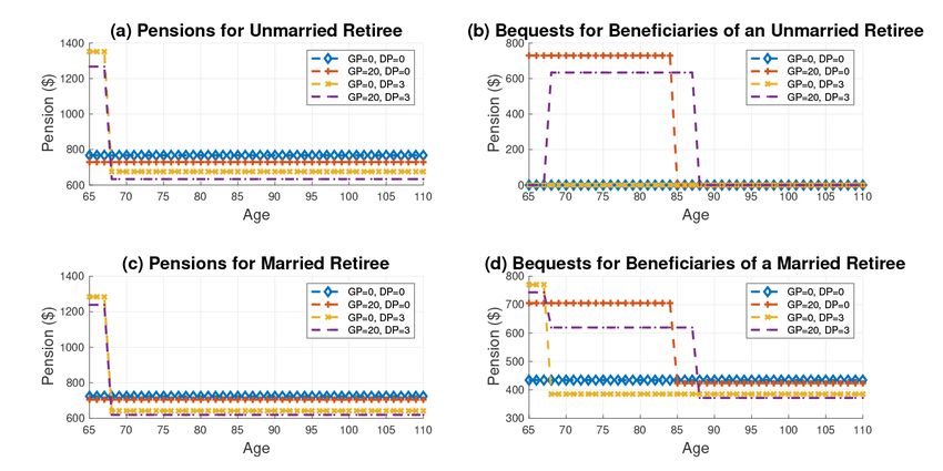
quintiles, on average, care 1.92 and 2.82 times more                       shutting down the role of risk ratings. Similar to the
about their spouse than themselves, respectively.                          complete information counterfactual, we find that using
                                                                           English auctions increases pensions for everyone.
Using our demographic information, we also estimate                        However, the gain is minimal for the retirees whose
the survival probability for each retiree. Comparing the                   savings belong to the lowest three quintiles. However, we
expected mortality with the model-implied annuitization                    find that these changes do not translate into large gains
costs, we find that retirees who may live longer                           in ex-post expected present discounted utilities because
have higher annuitization costs. We find significant                       either the increase is minimal (for those with lower
heterogeneity in these costs across retirees’ and across                   savings) or they increase (for those with high savings).
retirees’ savings. However, the average annuitization                      These retirees have higher pensions than other retirees,
costs do not increase with savings, despite the fact                       and because of diminishing marginal utilities, the utility
that in our estimation those with higher savings live                      gains from English auctions are minimal.
longer, which in turn is consistent with other studies
(e.g., Attanasio and Emmerson, 2003) that document a                       In the remainder of the paper we proceed as follows. In
negative correlation between wealth and mortality. The                     Section 2, we introduce the institutional detail; and in
average costs do not increase with savings quintiles                       Section 3, we describe our data. Section 4, presents
because for the top two quintiles with 0.14 probability,                   our model and Section 5 discusses its identification.
firms’ annuitization costs are less than actuarially fair                  Sections 6 and 7 present estimation and counterfactual
self-annuitization costs. This probability drops to 0.06 for               results, respectively and Section 8 concludes. The
the rest.                                                                  appendix includes additional details.

To quantify the effect of asymmetric information on                        2. Institutional background
pensions and retirees’ ex-post expected utilities, we
simulate the equilibrium pension under the assumption                      The Chilean pension system went through a major reform
that the firms observe each other’s annuitization costs                    in the early 1980s, when it transitioned from a pay-as-
while shutting down the risk ratings. We find that the                     you-go system to a system of fully funded capitalization
gap between the observed pensions and the complete-                        in individual accounts run by private pension funds
information pensions is the largest for retirees who                       (henceforth, AFPs). Under this system, workers must
belong to the top two savings quintiles.                                   contribute 10% of their monthly earnings, up to a pre-
                                                                           predetermined maximum (which in 2018 was U.S.
This result is even though low savers value risk                           $2,319), into accounts that are managed by the AFPs.6
ratings the most, and they stand to benefit the most.
However, our estimates suggest that because firms’                         Upon reaching the minimum retirement age—60 years
risk ratings are not too different, at least for the two                   for woman and 65 years for men—individuals can
most competitive firms, differences in costs are more                      request an old-age pension, transforming their savings
important in determining pensions than risk ratings’                       into a stream of pension payments. In this paper, we
preferences.                                                               focus only on those retirees who have savings in their
                                                                           retirement accounts, that are above a certain threshold,
Next, we evaluate the effect of replacing the current                      who can, and must, participate in the electronic annuity
pricing mechanism with simpler English auctions while                      market.7

6
     This maximum, and annuities in general, are expressed in Unidades de Fomento (UF), which is a unit of account used in Chile. UF follows the
     evolution of the Consumer Price Index and is widely used in long-term contracts. In 2018, the UF was approximately equivalent to U.S. $39.60.
7
     The threshold is currently established as the amount required to finance a Basic Solidarity Pension, which is the minimum pension guaranteed
     by the state. Retirees with insufficient funds will receive them from the AFP based on a programmed withdrawal schedule.

		                                                                                                          Auctioning annuities | March 2021       4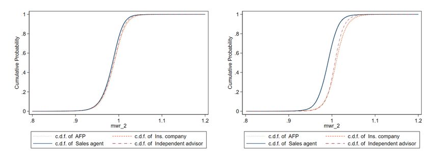
Regulation                                                                  volatility and provide no longevity insurance so that,
                                                                            barring extraordinarily high returns, the pension steadily
The Chilean government regulates and supervises AFPs,                       decreases over time.
who manage retirement savings during the accumulation
phase, and life insurance companies, who provide                            Under both IA and DA, the retiree’s savings are
annuities during the decumulation phase. In addition,                       transferred to an insurance company of her choice
at the time of retirement, the government provides                          that will provide an inflation-indexed monthly pension
subsidies to workers who fail to save enough during                         to her and her surviving beneficiaries. In deferred
their working years (Fajnzylber, 2018).                                     annuities, pensions are contracted for a future date
                                                                            (usually between one and three years), and in the
Moreover, the life insurance industry is heavily regulated.                 meantime the retiree is allowed to receive a temporary
The current regulatory frame-work for life insurance                        benefit that can be as high as twice the pension
companies providing annuities recognizes that the main                      amount.
risks associated with annuities are the risk of longevity
and reinvestment. Longevity risk is taken care of through                   Thus, the main trade-off between an annuity and a PW
the creation of technical reserves by insurers that sell                    is that an annuity provides insurance against longevity
annuities, which consider self-adjusting mortality tables.                  risk and financial risk whereas under a PW a retiree
The government also regularly assesses the risk of                          can bequeath all remaining funds in case of an early
reinvestment via the Asset Sufficiency Test established                     death. Moreover, while annuitization is an irreversible
in 2007. Under this regulation, every insurance company                     decision, a retiree who chooses a PW can switch and
is required to establish additional technical reserves, if                  choose an annuity at a later date.
and when there are “insufficient” asset flows, following
the international norm of good regulatory practices in                      Annuities may also include a special coverage clause
insurance industries. Bankruptcy among life insurance                       called a guaranteed period (GP).9 If an annuity includes,
companies is rare in Chile, but the government                              for instance, a 10-year guaranteed period, the full
guarantees every retiree pensions up to 100% of the                         pension will be paid during this period to the retiree,
basic solidarity pension, and 75% of the excess pension                     eligible beneficiaries or other individuals. Once the
over this amount, up to a ceiling of 45 UFs (see footnote                   guaranteed period is reached, the contracts reverts to
6). Thus, there are enough safety nets for retirees to feel                 the standard conditions (implying a certain percentage of
protected in case of a bankruptcy.                                          the original pension and only for eligible beneficiaries).10

2.1 Pension products                                                        For illustration of how benefits change with the annuity
                                                                            products and marital status, consider a male retiree who
Retirees participating in the electronic market have three
                                                                            is 65 years old, has a savings of U.S. $200,000 and is
main choices: programmed withdrawal (PW), immediate
                                                                            retiring in 2020. Suppose he is unmarried and chooses
annuity (IA), and deferred annuity (DA).8 Under PW,
                                                                            an annuity with GP=0 and DP=0, then he gets a constant
savings remain under AFP management and are paid
                                                                            pension until death (blue ‘◇’ in Figure 1-(a)), but after that
back to the retiree following an actuarially fair benefit
                                                                            his beneficiaries gets nothing (blue ‘◇’ in Figure 1-(b)).
schedule. In the event of death, remaining funds are
                                                                            But if he chooses an annuity with GP=20, then while alive
used to finance survivorship pensions or, in absence
                                                                            he gets lower pension (compare red ‘+’ and blue ‘◇’ in
of eligible beneficiaries, become part of the retiree’s
                                                                            Figure 1-(a)), but if he dies within 20 years of retirement,
inheritance. PW benefits are exposed to financial

8
     There is a fourth, rarely chosen, pension product which is a combination between a PW and an IA.
9
     Another rarely chosen clause is the spouse’s percentage increase, which maintains the full payment to the surviving spouse, instead of the
     mandated 50% or 60% for regular contracts.
10
     In our sample, 99.9% of the chosen annuities correspond to contracts with 0, 10, 15, or 20 years of GP.

		                                                                                                             Auctioning annuities | March 2021   5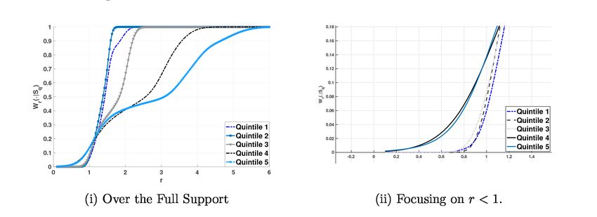
his beneficiaries get a strictly positive amount (purple                          DP=0 (blue ‘◇’ in Figure 1-(c)), the beneficiaries will get a
‘x’ in Figure 1-(b)) for 20 years, and after that they get                       positive amount (blue ‘◇’ in Figure 1-(d)) after the retiree
nothing. If he was married, then even with GP=0 and                              dies.

     Figure 1. Benefit schedules, by annuity type

     Note: The figure shows the survival-contingent benefit schedules for retirees and their beneficiaries for a
     representative retiree in our data, who is a 65-year-old male with savings of U.S. $200,000. Subfigures
     (a) and (b) shows the pension and bequest schedules, respectively, for four types of annuities and if he is
     unmarried. Similarly, subfigures (c) and (d), show the pension and benefit schedules when he is married. All
     calculations are performed by the authors using the offcial 2020 mortality table. GP stands for guaranteed
     period (in years) and DP stands for deferred period (in years).

2.2 Retirement process                                                           characteristics. Then the decision process can be
                                                                                 described in the following steps:
The process of buying an annuity begins when a worker
communicates her decision of considering retirement                              1. The retiree requests offers for different types of
to her designated AFP. We assume that she is then                                   pension products (described above).12 Upon request,
exogenously matched with one of four intermediaries or                              insurance companies in the system have eight
“channels” who can help her choose a product and firm.                              business days to make an offer (for every requested
                                                                                    annuity products).
Out of these four channels, two (AFP and insurance
                                                                                 2. These offers (i.e., bids) are collected and collated by
company) are free and the other two (sales agent and
                                                                                    the SCOMP system and presented to the retiree as
independent advisor) charge fees. Retirees must also
                                                                                    a Certificate of Quotes. The certificate is in the form
disclose information on all eligible beneficiaries.11
                                                                                    of a table, one for each type of annuity, sorted from
The AFP then generates a Balance Certificate that
                                                                                    the highest to the lowest pensions along with the
contains information about the total saving account
                                                                                    company’s name and risk-rating.13
balance (henceforth, just savings) and her demographic

11
        The main beneficiaries are the retiree’s spouse and their children under age 24.
12
        Retirees can request quotes up to 13 different variations, including PW and annuities with different combinations of contractual arrangements.
13
        In the case of guaranteed periods, the certificate also includes a discount rate that would be applicable in the event of death within the GP. In
        absence of legal beneficiaries, other relatives can receive the unpaid benefits in a lump sum, calculated with the offered discount rate. For an
        example see Figure 1.

		                                                                                                                 Auctioning annuities | March 2021        6
3. The retiree can choose from the following five                                   who used SCOMP to buy an annuity or choose PW
   options: (i) postpone retirement; (ii) fill a new                                during this period. As mentioned before, we observe
   request for quotes (presumably for different types                               everything about a retiree that participating life insurance
   of annuities); (iii) choose PW; (iv) accept one of the                           companies observe about them before they make their
   first round offers for a particular type of annuity; or (v)                      entry decisions and their first round offers. We observe
   negotiate with companies by requesting second round                              all the offers they received, their final choice, and
   offers for one type of annuity. In the latter case, firms                        whether they chose it in the first round or the second
   cannot offer lower than their initial round offers, and                          round. Our working assumption is that retirees use the
   the individual can always fall back to any first round                           first round offers to decide between different types of
   offer.14                                                                         annuities in most cases. Furthermore, conditional on
                                                                                    choosing the annuity type, they bargain with companies
3. Data                                                                             for better pensions in the second round.

We have data on the annuity market in Chile from                                    3.1 Retirees
January 2007 to December 2017. We observe everyone                                  .

     Table 1. Share of pension products
     Product                                           Obs.                             %
     PW                                              78,161                             32.7
     Immediate annuity                               87,115                             36.4
     Deferred annuity                                73,272                             30.6
     Annuity with PW                                    343                              0.9
     Full Sample                                   238,891                              100

     Note: The table shows the distribution of retirees across different annuity products. We restrict ourselves to
     annuities with either 0, 10, 15 or 20 years of guaranteed periods or at most 3 years of deferment.

We focus on individuals without eligible children                                   PW, immediate annuities, and deferred annuities: see
considering retirement within ten years of the “normal                              Table 1. Less than 1% of retirees choose annuity with
retirement age” (NRA), which is 60 years for a woman                                PW, and so we exclude them, leaving a total of 238,548
and 65 years for a man. The result is a data set with                               retirees.15
238,891 retirees, with an almost even split between

     Table 2. Age distribution, by gender and marital status
     Retiring Age                        S-F             M-F             S-M                M-M           Total
     Before NRA                          1,871           1,771           4,714            22,142         30,498
     At NRA                             20,789          22,475          17,114            72,572       132,950
     Within 3 years after NRA           14,470          16,797           4,447            19,086        54,800
     At least 4 years after NRA          6,900           6,715           1,251              5,434       20,300
     Full Sample                       44,030           47,758          27,526           119,234       238,548

     Note: The table displays the distribution of retirees, by their marital status, gender and their retirement ages.
     Thus the first two columns ‘S-F’ and ‘M-F’ refer, respectively, to single female and married female, and so on.
     NRA is the ‘normal retirement age,’ which is 60 years for a female and 65 years for a male.

14
          A firm that does not offer in the first round cannot participate in the second round.
15
          The fourth option allows retirees to split their savings into PW and annuity.

		                                                                                                                       Auctioning annuities | March 2021   7
In Table 2, we present the sample distribution by Retirees also vary in terms of their savings; see Table 3.
retirees’ marital status, gender, and age at the time of The mean savings in our sample is $112,471, while the
their retirement. Around 56% retire at their NRA, and median savings is $74,515 with an inter-quartile range of
79% retiree at or at most within three years after NRA $85,907. Savings are higher for men and for those who
(rows 2 and 3), and married men are half of all retirees. retire before NRA.
Table 3. Savings, by retirement age and gender
Mean Median P25 P75 N
Retiring Age
Before NRA 185,660 129,637 73,104 245,857 30,498
At NRA 89,907 60,023 41,521 103,680 132,950
Within 3 years after NRA 115,666 87,126 54,353 135,562 54,800
At least 4 years after NRA 141,673 101,594 58,815 168,202 20,300
Full Sample 112,471 74,515 46,449 132,356 238,548
Gender
Female 97,308 81,180 51,817 121,633 91,788
Male 121,955 69,372 43,818 147,184 146,760
Full Sample 112,471 74,515 46,449 132,356 238,548
Note: Summary statistics of savings, in U.S. dollars, by retiree’s age at retirement, and by retiree’s gender.
3.1.1 First round offers Moreover, there is also substantial variation in the
A retiree receives approximately 10.6 offers for several pensions offered across life insurance companies and
types of annuity, and the number of offers increases retirees; see Table 4. For an immediate annuity, retirees
with savings. For example, retirees with savings at the get an average offer of $570, and for deferred annuities,
75th percentile of our sample get an average of 12.4 the average offer is $446. On average, women get an
offers, and those at the 25th percentile get an average offer of $479 for immediate annuities and $412 for
of 7.8 offers. It is reasonable to assume that retirees deferred annuities, while for men, they are $631 and
with higher savings are more lucrative for the firms, and $473 respectively. These features are consistent with
therefore more companies are willing to annuitize their men having larger savings and shorter life expectancy
savings. If those with higher savings, however, also live than women (see Table 7).
longer than those with lower savings, then it means that
annuitizing higher savings is costlier for the firms. To
determine which of these two opposing forces dominate,
we estimate the annuitization costs and mortality by
savings.
Auctioning annuities | March 2021 8Table 4. Monthly pension offers, by annuity type and gender
Annuity Type Gender Mean Median Savings Q1 Savings Q2 Savings Q3 Savings Q4 Savings Q5
Immediate Female 479 414 202 288 385 510 857
Male 631 435 200 269 372 585 1329
Full Sample 570 423 201 278 378 556 1152
Deferred Female 412 374 190 258 349 463 714
Male 473 356 187 241 331 529 1019
Full Sample 446 365 189 248 339 500 882
Note: Summary of average monthly pensions (in U.S. dollars) offers received in the first round.
In our empirical model, we rationalize this variation in 3.1.2 Chosen annuities
pension offers by allowing firms to have heterogeneous Once the participating companies make first round
costs (UNCs) of annuitization. We assume that only the offers, one for each type of annuity the retiree requests
firm knows its annuitization cost, which can depend quotes for, she can either choose from one of those
on retirees’ savings. An important exogenous factor offers or buy a PW, or initiate the second round
affecting UNCs is the market interest rate, which affects bargaining phase. Table 5 displays the distribution across
the opportunity cost of offering a pension at retirement. these stages. Most retirees who choose PW choose that
Our sample spans a decade, so we observe substantial in the first round (98.1%), and most retirees (86.9%) who
variation in interest rates, which causes exogenous choose annuity choose in the second round. As we can
variation in annuitization costs. see, 2,979 retirees opt for the second round but choose
an annuity quote from the first round.
Table 5. Number of retirees who choose in first or second round
Round/Choice PW 1st round 2nd round Total
1 round
st
76,690 18,001 0 94,691
2nd round 1,471 2,979 139,407 143,857
Total 78,161 20,980 139,407 238,548
Note: Round refers to whether retirees chose in the first or second round.
In Table 6, we present information about the chosen (v) the percentage of retirees who requested at least
annuities: (i) the total number of accepted offers by the one second round offer; (vi) the percentage of retirees
type of annuity; (ii) the average number of first round and who chose the highest-paying alternative; and (vii) the
second round offers received for the chosen annuity; percentage of retirees who chose a dominated option, in
(iii) the number of accepted second round offers; (iv) the terms of either pension (with the same risk-rating) or risk
average percentage increase in pension offers from first ratings (with the same pension) or both.
round to second round (only for the accepted choice);
Auctioning annuities | March 2021 9Table 6. Summary of accepted annuities
Average # of Average %
GP # # Accepted in
1st round requested
Months Accepted 2nd round Increase Best Dominated
offers 2nd round
Immediate
0 21,292 11.3 16,357 1.5 80 59 22
120 26,907 11.1 23,463 1.3 89 51 28
180 24,452 11.6 22,070 1.4 92 49 29
240 14,464 11.8 13,020 1.5 92 51 29
Total 87,115 11.4 74,910 1.4 88 53 27
Deferred
0 11,703 10.9 8,919 1.5 79 53 23
120 26,119 11.0 23,390 1.4 91 46 31
180 26,775 11.4 24,324 1.4 92 42 34
240 8,675 11.0 7,864 1.3 92 42 34
Total 73,272 11.1 64,497 1.4 90 45 31
Note: The table shows the number of chosen annuities by type of product, the average number of first round offers received for the chosen annuity,
the number of accepted offers that resulted from second round offers, the average percentage increase between the first round and second round
offers (for the accepted choice), the percentage of individuals who requested at least one second round offer, the percentage of retirees who chose
the highest-paying alternative option and the percentage of individuals who chose an offer that was dominated by another alternative with same (or
better) credit rating.
From Table 6, we see that some retirees do not choose information about past defaults. Thus, in the case of
the annuity with the highest pension. One way to Chile this suggests that retirees should not care much
rationalize this behavior is to recognize that besides about the risk-rating. Finally, how does this trade-off vary
pensions, retirees also care about firms’ risk ratings. with preferences for bequests? To determine which of
After all, risk-rating is a proxy of financial health, and it is these countervailing forces dominate and how pensions
also widely advertised as such. A retiree can prefer lower and utilities would change under alternative market rules,
pensions from healthier firms to a higher pension from a later we estimate a structural model.
less healthy firm.
3.1.3 Mortality
This rationalization, however, begs the follow-up A determinant of annuity demand and supply is the
questions: Is there an objective (i.e., correct) trade- retiree’s expected mortality. We observe every retiree
off between pension and risk-rating, and should it when they entered our sample, i.e., their retirement
be homogeneous or vary across retirees? If it is age and their age at death if they die by the end of our
heterogeneous, should it increase or decrease with sample period. Using this information, we estimate a
savings? On the one hand, because of the regulation, mixed proportional hazard model (defined shortly below)
those with lower savings are less exposed to the risk of and use the estimated survival function to predict the
firms defaulting than those with higher savings; those expected life conditional on being alive at retirement.
with higher savings should care more about the risk
ratings than those with lower savings. On the other Let the hazard rate for retiree i with socioeconomic
hand, savings positively correlated with education, so characteristics Xi at time t ∈ R+, that includes i’s age,
those with higher savings will process publicly available
Auctioning annuities | March 2021 10gender, marital status, savings and the year of birth, be suggest a smaller hazard risk is associated with younger
= h(Xi) × ψ(t), cohorts, individuals who retire later, with females, those
who are married, and those with higher savings.16 Using
where mi is i’s realized mortality date, ψ(t) is the these estimates, we report the median expected lives,
baseline hazard rate. Furthermore, let the hazard by gender and savings quintile, and their standard errors
function ψ(t) be given by Gompertz distribution, such in Table 7. Overall, 50% of males expect to live until 86
that the probability of i’s death by time t is Fm(t; λi, ) years, and 50% of females expect to live until they are
= 1 − exp and let 94.9 years old. As we can see, those who have larger
savings also tend to live longer than those with lower
The identification of such a model is well established savings.
in the literature (Van Den Berg, 2001). The maximum
likelihood estimated coeffcients of the hazard functions
Table 7. Median expected life, by savings quintile
Savings Male Female Overall
Q1 85.15 93.80 86.89
(5.79) (6.03) (5.82)
Q2 85.86 94.24 87.64
(5.81) (6.06) (5.84)
Q3 86.45 94.83 88.23
(5.83) (6.09) (5.88)
Q4 87.62 95.48 89.40
(5.88) (6.12) (5.95)
Q5 90.87 97.25 93.52
(6.01) (6.21) (6.11)
Total 86.75 94.91 89.57
(5.82) (6.09) (5.94)
Note: The table shows the predicted median expected life at the time of retirement
implied by our estimates of the Gompertz mortality distribution. Standard errors are
reported in the parentheses.
3.2 Intermediary channels particularly relevant for sales agents, who receive their
intermediation fee only if the retiree chooses the sales
We observe retirees with one of the four intermediary
agent’s firm. In other words, it is possible and very likely
channels (AFP, insurance company, sales agent,
that those with a sales agent would appear to value
or independent advisor) to assist them with their
the non-pecuniary benefits of a company more than the
annuitization process. If and when such an intermediary’s
pecuniary benefits. We allow preferences for risk ratings
incentives do not align with those of a retiree, then
and information processing costs to depend on the
retirees do not always choose the “best” option
channel to capture this effect.
for them. The misalignment of incentives may be
16
For robustness, we estimated the Gompertz model using data from before the introduction of SCOMP. The estimates are qualitatively the same.
For instance, the predicted median expected life at death is 85 and 96 for males and females, respectively. Both of these results are available
upon request.
Auctioning annuities | March 2021 11To account for observed differences among retirees, insurance company, sales agent, advisor), are (0.989, we consider the money’s worth ratio (henceforth, mwr), 0.988, 0.984, 0.987) and (0.990, 0.989, 0.986, which is the expected present value of pension per 0.988), respectively, but the means and medians for annuitized dollar. If mwr = 1, then it means the retiree accepted offers are (1.010, 1.010, 0.990, 1.007) and expects to get $1 pension (in present value) for every (1.010, 1.009, 0.991, 1.007), respectively. Thus, the annuitized dollar. In Figure 2, we display the distributions final accepted offers are on average better than the first of the mwr offered in the first round (left panel) and round offers, and those with sales agents have lower mwr accepted by the retirees (right panel). The mean mwr. and the median mwr of the offers, by channels (AFP, Figure 2. CDFs of offered and accepted MWR, by channel Note: Distributions of the offered and chosen mwr (left panel vs. right panel), by channel. We use a multinomial logit model to consider if observed characteristics and the channel are correlated. For differences among retirees can explain the differences instance, those who have lower savings, retire early, are in their channels see; Table 8. In particular, we estimated male or unmarried are more likely to use sales agents the log-odds ratio of having one of the three intermediary than AFP. channels relative to the AFP and found that some Auctioning annuities | March 2021 12
Table 8. Intermediary channel - Estimates from multinomial logit
 Regressors\Channels                Insurance Company                 Sales-Agent                      Advisor
 Savings ($million)                     0.629***                      -0.857***                      -0.130***
                                         (0.128)                       (0.0436)                       (0.0447)
 Age                                     0.0131                      -0.0408   ***
                                                                                                    -0.0816***
                                      (0.00857)                      (0.00189)                      (0.00218)
 Female                                 0.437***                     -0.0588***                      -0.124***
                                        (0.0546)                       (0.0120)                       (0.0140)
 Married                                 0.0245                       0.0620   ***
                                                                                                     0.0874***
                                        (0.0491)                       (0.0107)                       (0.0127)
 Constant                              -5.029 ***
                                                                       2.333   ***
                                                                                                      4.326***
                                         (0.560)                        (0.123)                        (0.142)
 N                                      238,548                        238,548                        238,548

 Note. Estimates of multinomial logit regression for channels, where the baseline choice is AFP. Standard errors are in
 parentheses, and ***,** ,* denote p-values less than 0.01, 0.05 and 0.1, respectively.

We treat the channel as exogenous for model tractability.                     effects of potential selection based on unobservable
There are two reasons why we believe this is not as                           characteristics.
strong an assumption in our context as it might appear.
First, several anecdotal evidence from Chile suggests                         For instance, from Table 9, we see that channels affect
that most people rely on word-of-mouth when it comes                          the outcomes. Out of 109,786 retirees who choose
to a channel. Second, and as mentioned previously, we                         AFP, only 25.1% choose the second round, whereas
observe everything the firm observes about a retiree                           the shares are 85.2%, 92.0%, and 87.8% for insurance
when making the first round offers. When we estimate                           company, sales agents, or advisors, respectively. Most
the preference parameters, we estimate them separately                        of those who choose PW have AFP, and those with sales
for several groups that we define based on age, gender,                        agents are least likely to choose PW.
savings, and channels. Estimating preference parameters
separately for each group allows us to control the

 Table 9. Retiree choices, by intermediary channel
                               N                Requests 2nd Round            Chooses PW        Chooses in 2nd Round
 AFP                     109,786                     0.251                     0.661                  0.235
 Company                    2,169                    0.852                     0.066                  0.817
 Sales-agent               79,120                    0.920                     0.030                  0.907
 Advisor                   47,473                    0.878                     0.066                  0.846
 Full Sample             238,548                     0.603                     0.328                  0.584

 Note: Proportion of retirees separated by their choices and their channel.

		                                                                                                            Auctioning annuities | March 2021 13
Our empirical framework can capture the effect of The ratings mostly remain the same over time, and most
channels on outcomes. In particular, we posit that companies have high (at least AA) risk ratings. For our
channels affect the cost of acquiring information about empirical analysis, we treat these ratings as exogenous,
the importance of risk-rating. For instance, we allow and group them into three categories: 3 for the highest
those retirees who use sales agents to act “as if” they risk rating of AA+, 2 for all the risk ratings from AA to A,
have a higher cost of acquiring information about the and 1 for the rest.
trade-off between risk-rating and pensions. We assume
that in the first stage, retirees are rationally inattentive Although there are 20 unique firms, not all of them
with respect to their preference for risk ratings, but they are active at all times, and not all participate in every
know their preferences in the second stage. auction. On average, 11 companies participate in
a retiree auction, which suggests that the market
3.3 Firms is competitive. We define potential entrants (for
In our sample, we observe 20 unique life insurance each retiree auction) as the set of active firms that
companies, and they differ in terms of their annuitization participated in at least one other retiree auction in the
costs, which are unobserved, and in terms of their risk same month. In our sample, retirees have either 13, 14,
ratings. Table 10 shows the distribution of risk ratings. or 15 potential entrants.
Table 10. Risk ratings
Rating Frequency % Cumulative %
AA+ 155 24.64 24.64
AA 245 38.95 63.59
AA- 171 27.19 90.78
A+ 2 0.32 91.1
A 15 2.38 93.48
BBB+ 1 0.16 93.64
BBB 6 0.95 94.59
BBB- 15 2.38 96.98
BB+ 19 3.02 100
Total 629 100
Note: The table shows the distribution of quarterly credit ratings from 2007-2018.
The participation rate, which is the ratio of the number retirees.18 To capture this selection, in our empirical
of actual bidders to the number of potential bidders, application, we follow Samuelson (1985) to model firms’
varies across our sample from as low as 0.08 to as high entry decisions, which posits that firms observe their
as 1, with mean and median rates of 0.73 and 0.78, retiree-specific annuitization cost before entry. This
respectively, and a standard deviation of 0.18.17 Thus, entry method is a reasonable assumption in our setting
it is likely that a firm’s decision to participate depends because firms have sophisticated models to predict
on its financial position when a retiree requests quotes retirees’ mortality and the expected returns from the
and this opportunity cost of participating can vary across savings.
17
Using a Poisson regression of the number of participating firms on the retiree characteristics, we find that one standard deviation increase
in savings, which is approximately $87,000, is associated with roughly one more entrant. Moreover, women have 0.61 more participating
companies than men, while sales agents and advisors are associated with approximately 0.19 fewer participants than the other two channels.
18
We tested this selection by estimating a Heckman selection model with the number of potential bidders as the excluded variable and found
strong evidence of negative-selection among firms.
Auctioning annuities | March 2021 14We treat firms as symmetric bidders with annuitization using ordinary least squares method, and predict
costs independently and identically distributed with some the residual εˆi,j for retiree i and firm j. In Figure 4,
(unknown) distribution function. We do not observe firms’ we show the Kernel density estimate of the firm-
annuitization costs, and so, we cannot directly test this specific distribution of ˆε i,j. We can see that these 20
assumption. However, we can per-form a diagnostic test distributions are very similar, so it is reasonable to say
and check if the firm-specific pension (bid) distributions that firms have symmetric cost distribution.
are different. If they are not different from one another,
then our symmetry assumption is a reasonable first step. 4. Model
However, to perform this test, we have to “control” for In this section, we introduce our model. To model the
all relevant factors that can affect the pension. For demand, we consider the decision problem facing
instance, retirees with high savings can be lucrative a retiree who uses SCOMP to choose a company
because the total gain from annuitizing their savings to annuitize her savings. To model the utility from
will be large. However, as we have seen above, these an annuity, we closely follow the extant literature
retirees are expected to live longer. To compare the on annuities, particularly, Einav, Finkelstein, and
bids across firms,we have to estimate the expected Schrimpf (2010), with a modification that accounts for
discounted life for each retiree, which we refer to as heterogeneous preferences for firm characteristics.
UNCi where the subscript i refers to retiree i. This UNCi
is different from UNCj, where the latter refers to a firm As we have shown before, retirees do not always choose
j’s cost. We formally define UNCi when we present our the best offer. To rationalize this, we posit that besides
model’s supply side, and in Appendix A.1 we detail how the pecuniary aspect of an annuity, retirees also care
we use the estimates from the mortality distribution to about a company’s risk ratings, which is a proxy for
calculate UNCi. But for now, it is sufficient to know that the likelihood of default. That said, we assume that
UNCi depends on i’s estimated mortality and the discount all retirees have a prior that puts much emphasis on
factor. A retiree who expects to live longer will have a risk-rating, and only those who spend some resources
larger UNCi and will be costlier for firms to annuitize, but learning about the likelihood of default will update their
these costs are unobserved. prior and choose accordingly. To capture the trade-off
between pension, risk ratings, and information gathering,
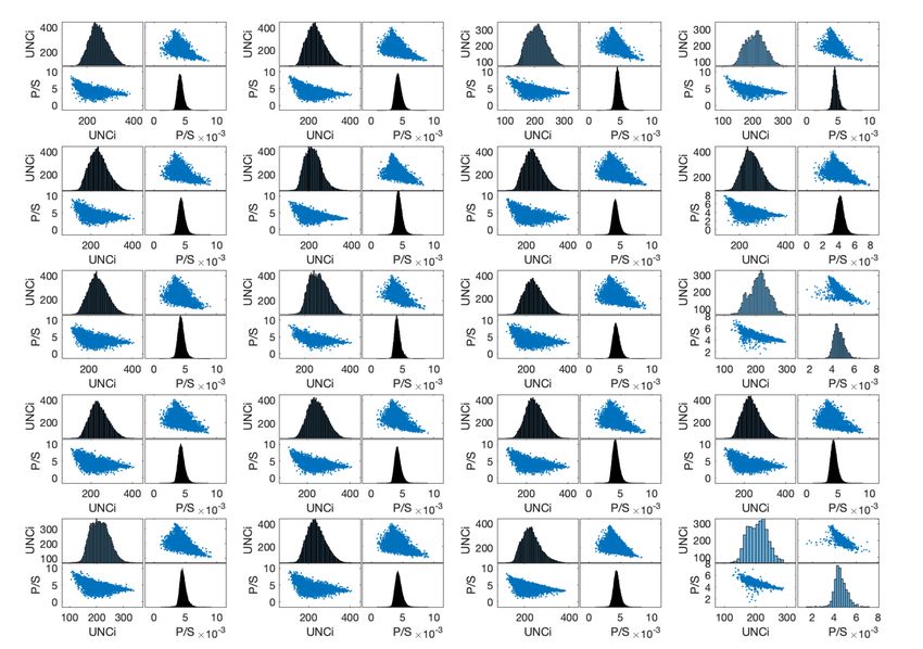
For each of the 20 firms, in Figure 3 we present the we follow Matëjka and McKay (2015) and model the
histograms and scatter plots of monthly pension per retiree as a rationally inattentive decision maker. If a
annuitized dollar (which is known as the monthly pension retiree chooses to go to the second round bargaining,
rate) and the UNCis of all the retirees that the firms make we assume that she knows her risk ratings preferences.
offers to in the first stage. Using pension rates instead of
pensions allows us to compare across different retirees.
As we see, indeed UNCi and pension rates are negatively
correlated, and there are no differences across firms.
Now, using these UNCis, we can compare pensions across
firms. We normalize the offered pension rates (ratio of
monthly pension to annuitized savings) across firms,
and compare the distributions across firms. We say that
firms are asymmetric if the distributions are different and
symmetric otherwise. For each firm we estimate
Auctioning annuities | March 2021 15Figure 3. Pension rates and UNCi for each firm Note: These are histograms and scatter plots of monthly pension rate, i.e., the ratio of monthly pension to annuitized savings, and the UNCi of the retirees the firms make an offer. There are 20 firms, so there are 20 sets of four subfigures each. Clockwise, the first subfigure is the histogram of UNCi, and the second subfigure is the scatter plot of the pension rates (on the x-axis) and UNCi (on the y-axis). The third subfigure is the histogram of the pension rates, and the last subfigure is the scatter plot of UNCi and the pension rates. On the supply side, we model the imperfect competition sided asymmetric information. The winner of the game using an extensive form game where the first stage is not always the firm that offers the highest pension is a first-price auction with independent private value because the probability of winning depends on the bids and endogenous entry (Samuelson, 1985). If there is a and the preferences for risk-rating and bequest, which second stage, then it is multilateral bargaining with one- can vary across retirees. Auctioning annuities | March 2021 16
Figure 4. Distributions of homogenized pension rates, by firms

 Note: Kernel estimates of the distribution residuals εˆ ij from Equation (1), one for each firm.

4.1 Demand                                                                     and therefore will act as someone who does not care
                                                                               about bequest we allow         to have a mass point at θ
Here, we consider the problem faced by an annuitant
                                                                               = 0. Letting ζ ∈ (0, 1) be the probability that the retiree
i who has already decided which annuity product to
                                                                               has θi = 0, and let Fθ (·) = ζ × H(0) + (1−ζ) × (·) where,
choose (e.g., an immediate annuity with 0 guaranteed
                                                                               H(0) is a Heaviside function and        is the continuous
period) and is considering between Ji firms who have
                                                                               distribution on
decided to participate in the auction for i’s savings Si.
The retiree will choose the firm that provides her the
                                                                               Let Pij denote the pension offered by firm j to
highest indirect utility.
                                                                               retiree i. Given the type of annuity and the pension
                                                                               Pij, i’s expected mortality and the mortality of her
We assume that the utility from an annuity consists of
                                                                               beneficiaries determine the bequest, which we denote
three parts: the expected present discounted utility from
                                                                               by Bij(Pij). Whenever it is clear from the context, we
the monthly pension that the retiree enjoys while alive,
                                                                               suppress the dependence of Bij on Pij. Let i’s indirect
utility she gets from leaving bequest (if any) to her kin,
                                                                               utility at retirement from choosing an annuity with
and her preference for firm’s risk rating. Retirees may
                                                                               pension and bequest (Pij, Bij) from firm j with risk rating
value the risk ratings because they may dislike firms
                                                                               Zi,j ∈ {1, 2, 3} be
with lower risk ratings. However, they may not know
the “correct” weight to put on these risk ratings. To
capture this uncertainty, we model retirees as rationally
inattentive decision makers. We explain this aspect
                                                                               where the utility        is the utility associated with the
shortly below, but for ease of exposition, we begin
                                                                               outside option.
without rational inattention.
                                                                               Next, we explain the expected present discounted
Let (θi, βi) denote i’s preferences for bequest and risk-
                                                                               utility,            For simplicity, consider only the first
rating, respectively, and given savings S are distributed
                                                                               month after retirement, and let qi be the probability
independently and identically across retirees as
                                                                               of being alive one month after retirement. Then, the
                    on               To capture the fact
                                                                               expected present discounted utility will be
that retirees might not be able to afford bequest,

		                                                                                                        Auctioning annuities | March 2021 17
where u(Pij) is the utility from Pij, and v(Bij) is the utility of months that the spouse (or other beneficiaries) will
from leaving a bequest Bij. Thus, the marginal utility from receive the full pension because of the guaranteed
leaving a bequest Bij upon death is θi × (1 − qit) × v'(Bij). period. Furthermore, is the discounted number of
Now, let us consider two periods after retirement. We months that the spouse will receive 60% of the retiree’s
have to adjust the probability that the retiree survives pension.19 If the annuity has a deferred period, then the
two periods given that she is alive at retirement and take retiree gets twice her pension until the annuity payment
into account that the bequest left upon death will also begins. So where
change, which in turn depends on whether the annuity is the expected life during the deferred period.20
product under consideration includes a guaranteed
period. However, a retiree can have additional wealth, besides Si,
that she can use for consumption or bequest, especially
In practice, we do not know for how long i expects to live. those who are wealthy. However, we do not observe her
So, to determine expected longevity at retirement, we consumption (after retirement) or her wealth, so following
estimate a continuous-time Gompertz survival function the literature (Mitchell et al., 1999; Einav, Finkelstein,
for i and her spouse (if she is married) as a function of and Schrimpf, 2010; Illanes and Padi, 2019), we assume
her demographic and socioeconomic characteristics. that retirees have homothetic preferences. In particular,
Once we have the survival probabilities, the expected we assume that all retirees have CRRA utility
discounted utilities become the product of u(Pij) and the with γ = 3. Homothetic preferences
discounted number of months i expects to live, where the imply that the retiree’s annuity choice does not depend
discount factor is the market interest rate. on the unobserved wealth. In Appendix A.1, we detail the
steps to estimate ρi(Pij) and bi(Pij).
Even with a bequest, has an intuitive
structure. It is a sum of two terms, one of which is the Substituting (3) in (2) we can express i’s indirect utility
product of u(Pij) and the discounted number of months i from annuity Pij from firm j as
expects to live, and the other term is the product of v(Bij)
times the discounted number of months i’s beneficiaries
expect to receive Bij. Legally, i’s spouse is entitled to
60% of i’s pension, and 100% during the guaranteed Thus, (4) shows that there is a trade-off between higher
periods; the amount Bij may change over time. pensions and lower risk ratings, but as mentioned above,
we assume that i does not know her βi, but only its
Thus, we can write as distribution.
We follow Matëjka and McKay (2015) and assume that
before the retirement process begins, i has a belief that
with support and if i wants to learn
where is the discounted expected longevity of her preference, she has to incur information processing
the retiree (in months, from the moment the annuity cost, valued at α > 0 per unit of information. So, i has
payments start) and is the discounted number first to decide how much to spend learning about βi, and
19
These “discounted life expectancies” also have interpretation in terms of the annuitization costs. Assuming firms use the same mortality
process as us and invest retirees’ savings at an interest rate equal to the discount rate, then is the necessary capital to provide a one-
dollar pension to the retiree until she dies. Similarly, is the necessary capital to finance a dollar of pension for the beneficiaries once the
retiree is dead and until the guaranteed period expires. Finally, is the necessary capital to finance a dollar of pension for the beneficiaries
between the retiree’s death or the guaranteed period is over (whichever occurs later) and until the spouse dies. The gains from trade between
retirees and insurance companies come from the differences in risk-attitude between retirees and life insurance companies and potential
differences between the discount rate of retirees and firms’ investment opportunities.
20
For simplicity, we are disregarding survival benefits during the deferment period. Deferred periods in our sample are at most three years. Thus,
death probability is quite low.
Auctioning annuities | March 2021 18after that make the decision. Let σ : cost of a pension calculated with the retirees’ discount
denote the strategy of a retiree with preference rate and the mortality process we estimate. For the
parameter β, with offered pensions Pi : = (Pi1, . . . , PiJ) ∈ . same retiree i, firms’ UNCs may differ from UNCi due
The strategy is a vector σ(β, Pi) ≡ (σ1(β, Pi), . . . , σJ (β, Pi), to the differences in their (i) mortality estimates, (ii)
σJ+1(β, Pi)) of probabilities, where σj(β, Pi) = Pr(i chooses investment opportunities, and (iii) expectations about
j|β, Pi) ∈ [0, 1]. For notational simplicity, we suppress future interest rates. For these reasons, it is more
the dependence of choice probabilities on the offers (Pi). likely that only firm j knows its UNCj . Moreover, the
Then, by adapting Matëjka and McKay (2015)’s choice ratio of UNCj to UNCi captures j’s relative efficiency
formula to two periods, the probability that i chooses j is selling an annuity to i. Henceforth, we call this ratio
given by j’s relative cost of annuitizing a dollar.
Working with r, we can compare retirees who otherwise
will have different UNCi ’s.
We assume the cost rij is private and is distributed
independently and identically across companies as
Wr (·|S), with density wr (·|S) that is strictly positive
4.2 Supply
everywhere in its support Thus, we assume
Next, we present the supply side, where J insurance that firms are symmetric, and this is consistent with
companies participate in an run by “auctioneer” i with what we observe in the data; Figure 4. Allowing the
characteristics Xi ≡ For simplicity, we suppress cost distribution to depend on S captures the fact that
the dependence on Xi and treat J as fixed, but account for those who have higher savings tend to live longer and,
selection in our empirical application. therefore, are costlier to annuitize.
Companies differ in terms of their UNCs. Thus, if j can Ignoring for now the second round, and the multi-product
annuitize i cheaper than j', then j has an advantage over nature of the first round, j’s net present expected profit
j' because all else equal, j can offer a higher pension. from offering Pij, to a retiree i with Si
Let be j’s unitary necessary capital to finance a
dollar pension for the retiree. Similarly, we must consider
the costs related to the bequest, which may come from
two sources: a guaranteed period, during which after
the death of the retiree the beneficiaries receive the where is the money worth ratio
full amount of the pension, and the compulsory survival (mwr) computed using the retirees’ discount rate, and
benefit, according to which the spouse of the retiree σij(Pi) is the probability that i chooses j given the vector
receives after the retiree died and after the guaranteed of offers Pi. Considering the second round, and denoting
period is over, 60% of the pension until death, see by the second round offer of firm j
Equation (A.1). We denote by and the
present value of the cost of providing these two benefits.
Then, j’s expected cost of offering Pij is
is its ex-ante expected profit, where σiJ+1(Pi) from (5) is
the probability that i takes the bargaining option in the
second round with expected profit given by
Here, the 2 in (6) follows from our assumption that the The two rounds are connected. First, more generous
life insurance company made the pension payments offers on the first round may lower the retiree’s
during the deferred period. Let UNCi be the unitary probability of going to the second round. Second, and
more importantly, each firm’s first round offer is binding
for the second round: A firm cannot make any second
Auctioning annuities | March 2021 19You can also read