Assessing vehicle fuel efficiency using a dense network
←
→
Page content transcription
If your browser does not render page correctly, please read the page content below
Research article
Atmos. Chem. Phys., 22, 3891–3900, 2022
https://doi.org/10.5194/acp-22-3891-2022
© Author(s) 2022. This work is distributed under
the Creative Commons Attribution 4.0 License.

        Assessing vehicle fuel efficiency using a dense network
                         of CO2 observations
            Helen L. Fitzmaurice1 , Alexander J. Turner2 , Jinsol Kim1 , Katherine Chan3 , Erin R. Delaria4 ,
                          Catherine Newman4 , Paul Wooldridge4 , and Ronald C. Cohen1,4
                       1 Department of Earth and Planetary Science, University of California Berkeley,
                                                 Berkeley, CA 94720, USA
                 2 Department of Atmospheric Sciences, University of Washington, Seattle, WA 98195, USA
                    3 Program Coordination Division, Sacramento Metro Air Quality Management District,

                                                Sacramento, CA 95814, USA
                   4 Department of Chemistry, University of California Berkeley, Berkeley, CA 94720, USA

                                Correspondence: Ronald C. Cohen (rccohen@berkeley.edu)

                                 Received: 28 September 2021 – Discussion started: 5 October 2021
                        Revised: 23 January 2022 – Accepted: 10 February 2022 – Published: 24 March 2022

       Abstract. Transportation represents the largest sector of anthropogenic CO2 emissions in urban areas in the
       United States. Timely reductions in urban transportation emissions are critical to reaching climate goals set
       by international treaties, national policies, and local governments. Transportation emissions also remain one
       of the largest contributors to both poor air quality (AQ) and to inequities in AQ exposure. As municipal and
       regional governments create policy targeted at reducing transportation emissions, the ability to evaluate the
       efficacy of such emission reduction strategies at the spatial and temporal scales of neighborhoods is increasingly
       important; however, the current state of the art in emissions monitoring does not provide the temporal, sectoral, or
       spatial resolution necessary to track changes in emissions and provide feedback on the efficacy of such policies
       at the abovementioned scale. The BErkeley Air Quality and CO2 Network (BEACO2 N) has previously been
       shown to provide constraints on emissions from the vehicle sector in aggregate over a ∼ 1300 km2 multicity
       spatial domain. Here, we focus on a 5 km, high-volume, stretch of highway in the San Francisco Bay Area.
       We show that inversion of the BEACO2 N measurements can be used to understand two factors that affect fuel
       efficiency: vehicle speed and fleet composition. The CO2 emission rate of the average vehicle (in grams per
       vehicle kilometer) is shown to vary by as much as 27 % at different times of a typical weekday because of changes
       in these two factors. The BEACO2 N-derived emission estimates are consistent to within ∼ 3 % of estimates
       derived from publicly available measures of vehicle type, number, and speed, providing direct observational
       support for the accuracy of the EMission FACtor model (EMFAC) of vehicle fuel efficiency.

1   Introduction                                                   represents the greatest sectoral percentage (∼ 25 %–66 %) of
                                                                   emissions from within the boundaries of urban areas in the
Urban emissions currently account for ∼ 75 % of all anthro-        United States (City of Oakland, 2020; Gurney et al., 2021).
pogenic CO2 emissions (Seto et al., 2014). By 2050, roughly        Although the fuel efficiency of new internal combustion en-
two-thirds of the Earth’s projected population of 9.3 billion      gine vehicles has increased by ∼ 30 % over the last 20 years,
is expected to reside within urban areas (Seto et al., 2014),      and electric vehicles (EVs) are becoming more prevalent
meaning that effective greenhouse gas (GHG) emission re-           (e.g., https://arb.ca.gov/emfac/emissions-inventory, last ac-
duction strategies must focus on urban emission reductions.        cess: 12 January 2022), emission reductions resulting from
   The transportation sector is responsible for ∼ 23 % of          fuel efficiency gains in newer vehicles are negated by an in-
global GHG emissions worldwide (Seto et al., 2014) and

Published by Copernicus Publications on behalf of the European Geosciences Union.
3892                 H. L. Fitzmaurice et al.: Assessing vehicle fuel efficiency using a dense network of CO2 observations

creasing percentage of heavy-duty vehicles (HDVs) (Moua,              However, even the most detailed of these inventories do
2020), speed-related reductions in fuel efficiency resulting       not presently describe the temporal variability in processes
from increases in congestion, and an increase in the total ve-     that affect emissions, such as the direct response of home
hicle kilometers traveled. Over the past 20 years, even in lo-     heating or air conditioning to ambient temperature or, with
cations with aggressive climate change policies, these fac-        one exception (Gately et al., 2017), the variations in emis-
tors have resulted in CO2 emissions from vehicles that have        sions per kilometer when comparing free-flowing with stop-
increased or stayed nearly constant. For example, the Cali-        and-go traffic. These models often disagree with one another
fornia Air Resources Board estimates that per capita vehicle       spatially (Gately and Hutyra, 2017), have been subject to
emissions in the state of California in 2015 were only 2 %         only limited testing against observations of the atmosphere,
lower than in 2000, and per capita vehicle kilometers trav-        and are not designed to be consistent with separately con-
eled increased ∼ 2.5 % over that time period (California Air       structed AQ inventories that have been subject to much more
Resources Board, 2018). In addition to GHG emissions, the          extensive testing against observations.
transportation sector is responsible for a significant share of       Mobile monitoring campaigns and high-density mea-
fine particulate matter (PM2.5 ) and NOx emissions, exacer-        surement networks highlight the importance of character-
bating PM2.5 and ozone exposure in BIPOC already experi-           izing and identifying the processes contributing to sharp
encing disproportionate health burdens associated with poor        neighborhood-scale AQ and GHG hot spots and point to the
air quality (Tessum et al., 2021).                                 importance of traffic emissions at neighborhood scales. For
   Municipal and regional governments have increasingly            example, Apte et al. (2017) showed that concentrations of
shown interest in tracking and reducing CO2 emissions from         NOx and black carbon (BC) can vary by as much as a fac-
all sectors, including transportation. For example, Boswell et     tor of ∼ 8 on the scale of tens to hundreds of meters. Caubel
al. (2019) found that 64 % of Californians live in a city with     et al. (2019) showed BC concentrations to be ∼ 2.5 times
a climate action plan. For urban and regional governments          higher on trucking routes than on neighboring streets. Such
to plan, monitor, and responsively adjust emission reduction       gradients are not represented in inventories based on down-
policies, an up-to-date understanding of the spatial and tem-      scaled economic data.
poral variations in total emissions and in emissions by sector        Observations of CO2 and other GHGs can play an impor-
and subsector processes is key.                                    tant role in improving and maintaining the accuracy of emis-
   For transportation, reductions in vehicle kilometers, con-      sion models – especially during a time of rapid proposed
gestion mitigation, and rules affecting fleet composition          changes. CO2 measurements paired with Bayesian inverse
(e.g., limiting road access to HDVs, incentivizing use of elec-    models have been shown to provide a quantitative assess-
tric vehicles, or buy-backs of older vehicles) are three levers    ment of emissions (Lauvaux et al., 2016, 2020; Turner et
that can be employed to reduce CO2 and AQ emissions from           al., 2020a). To date, most attempts at quantifying urban CO2
vehicles, thereby affecting the climate footprint, air quality     emissions have focused on extracting a temporally averaged
(AQ), and environmental justice (EJ) in a region. However,         (often a full year) total of the anthropogenic CO2 across the
the current state of the art in emission monitoring and model-     full extent of city. A few studies have attempted to disag-
ing do not provide the temporal, sectoral, or spatial resolution   gregate emissions by sector or fuel type or to describe large
necessary to track changes in urban emissions and provide          shifts in aggregate emissions (Newman et al., 2016; Nathan
feedback on the efficacy of each lever separately. Further-        et al., 2018; Lauvaux et al., 2020; Turner et al., 2020a), but
more, current estimates of the magnitude and sectoral appor-       none characterize the subsector processes of vehicle emis-
tionment of urban CO2 emissions can vary widely. For ex-           sions.
ample, Gurney et al. (2021) show how a consistent approach            High-spatial-density observations offer promise as a
to total emissions from cities across the United States differs    means to explore process-level emission details. The BErke-
from locally constructed inventories in magnitude and sector       ley Air Quality and CO2 Network (BEACO2 N) is an observ-
by sector.                                                         ing network deployed in the San Francisco Bay Area and
   Spatial and temporal process-level maps of emissions are        other cities with a measurement spacing of ∼ 2 km (Fig. 1,
needed to improve the scientific basis for emission control        left). In a prior analysis, Turner et al. (2020a) showed that
strategies. The current state of the art involves finding ag-      BEACO2 N measurements can detect variation in CO2 emis-
gregate emissions over large regions (e.g., counties or states)    sions with time of the day and day of the week in addition to
using economic data and then downscaling those totals us-          the dramatic changes in CO2 emissions due to the COVID-
ing proxies such as road length, building type, or population      related decrease in driving.
density. These models meet the need for high spatial reso-            Here, we analyze hourly, spatially allocated CO2 emis-
lution (∼ 500 m) and capture emissions from many detailed          sions derived from the inversion of BEACO2 N observations
subsectors (Gately et al., 2015; Gurney et al., 2012; McDon-       (Turner et al., 2020a) to explore how well they constrain the
ald et al., 2014). Because fuel sales are well characterized,      CO2 emissions from a 5 km stretch of highway. This stretch
these models are also likely to produce accurate region-wide       was chosen because of its location upwind of consistently
CO2 emission totals from the transportation sector.                active BEACO2 N sites, for completeness of traffic data, and

Atmos. Chem. Phys., 22, 3891–3900, 2022                                             https://doi.org/10.5194/acp-22-3891-2022
H. L. Fitzmaurice et al.: Assessing vehicle fuel efficiency using a dense network of CO2 observations 3893
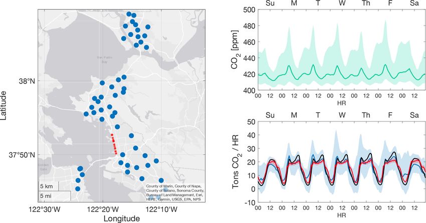
Figure 1. The left panel presents a map of the BEACO2 N network, showing all sites (blue dots) for which there are more than 4 weeks of
data during the period analyzed (January to June from 2018 to 2020). Red stars indicate the location of the PeMS monitors used in this study.
The top right panel presents CO2 values shown for a “typical week” during the time period observed. The dark line represents the median
value observed across all sites and times, and the shaded envelope represents 1σ variance across the network and over the 2-year period. The
bottom right panel presents CO2 emissions on all highway pixels in the domain as derived from the inversion of BEACO2 N observations
(blue), BEACO2N prior (black), and the PeMS-EMFAC-based estimate (red). The shaded envelope shows variance in emissions during the
18-month analysis window.
because emission rates are highly affected by speed (vehicles 17. Figure 1 shows sites in operation at some point during
use more fuel per kilometer at very low and high speeds) and analysis period, and Fig. S1 in the Supplement shows a time
fleet composition (HDVs emit more CO2 per kilometer than series of the number of nodes available throughout the study
light-duty vehicles, LDVs). The variation in the ratio of total period.
fleet CO2 emissions per vehicle kilometer traveled (grams of
CO2 per vehicle kilometer) is used to explore variations in
2.2 The BEACO2 N Stochastic-Time Inverted
on-road fuel efficiency and the factors responsible for that
Lagrangian Transport inversion system
variation. We show that the average fuel efficiency of the ve-
(BEACO2 N-STILT)
hicle fleet on the road varies by as much as 27 % over the
course of a typical weekday. To infer CO2 emissions from within the BEACO2 N foot-
print, we use the Stochastic-Time Inverted Lagrangian Trans-
port (STILT) model, coupled with a Bayesian inversion as
2 Methods and data
described in detail in Turner et al. (2020a). Briefly, we
2.1 The Berkeley Air quality and CO2 Network use meteorology from the National Oceanic and Atmo-
spheric Administration (NOAA) High-Resolution Rapid Re-
We use hourly CO2 observations from the Berkeley Air qual- fresh (HRRR) product at a 3 km resolution to calculate foot-
ity and CO2 Network (BEACO2 N) (Shusterman et al., 2016; prints from each hour at each site, weighted by a priori
Kim et al., 2018; Delaria et al., 2021). The BEACO2 N net- CO2 emissions. The overall region of influence, the net-
work includes more than 70 locations in the San Francisco work footprint, as defined by a contour representing 40 %
Bay Area, spaced at ∼ 2 km, and measures CO2 with a net- of the CO2 influence, is shown in Fig. S2 (left). We con-
work instrument error of 1.6 ppm or less (Delaria et al., struct a spatially gridded prior emission inventory using point
2021). All available data from January to June during the sources provided by the Bay Area Air Quality Management
2018–2020 period are included in this analysis. During this District (BAAQMD) (2015), home heating emissions as re-
time, more than 50 distinct locations had nodes that were ac- ported by BAAQMD (2011) and distributed spatially accord-
tive for a month or more (including 19 sites within 10 km of ing to population density, on-road emissions from the High-
our highway stretch of interest). The number of nodes ac- resolution Fuel Inventory for Vehicle Emissions (McDonald
tive at any given time ranged from 7 to 41, with a mean of et al., 2014) varying by hour of week and scaled by year us-
https://doi.org/10.5194/acp-22-3891-2022 Atmos. Chem. Phys., 22, 3891–3900, 20223894 H. L. Fitzmaurice et al.: Assessing vehicle fuel efficiency using a dense network of CO2 observations
ing fuel sales data, and a biogenic inventory derived using the PeMS network in comparison to the BEACO2 N-STILT
solar-induced fluorescence (SIF) satellite data (Turner et al., footprint as well as the total HDV vehicle kilometers and the
2020b). total LDV vehicle kilometers.
To ensure a focus on highway emissions, we subtract prior Vehicle fuel efficiency is dependent on both fleet compo-
estimates associated with non-highway sources from pos- sition and vehicle speed. We calculate an emission rate at
terior BEACO2 N-STILT fluxes. Non-highway sources are each location by combining the speed and the HDV per-
small (∼ 12 %) in comparison with highway emissions for centage with fuel efficiency estimates provided by the Cal-
the pixels corresponding to the highway stretch analyzed in ifornia Air Resources Board EMission FACtor model (EM-
this study (Fig. 2, left). We assume the error in prior esti- FAC2017). The EMFAC2017 model provides yearly fuel ef-
mates of these sources to be an even smaller fraction of the ficiency estimates for the San Francisco Bay Area for 41 ve-
total. For reference, a diel cycle of sector-specific, weekday hicle classes as a function of speed. We group these 41 ve-
prior emissions for the pixels analyzed in this study is shown hicle types into the LDV or HDV categories (Table S1). The
in Fig. S3. PeMS vehicle-type classification system is length based, as-
We estimate the BEACO2 N-STILT inversion to be precise suming that LDVs have a median length of 3.7 m and HDVs
to at least 30 % for a line source. This estimate is based on have a median length of 18.3 m (Kwon et al., 2003). As a
the results of Turner et al. (2016), who used observation sys- result, we group most light-duty trucks into the LDV cat-
tem simulation experiments to demonstrate that a 45 tC h−1 egory. To find speed-dependent emission rate values for the
line source could be constrained to 15 tC h−1 with 7 d of ob- LDV and HDV groups, we find a vehicle-kilometer-weighted
servations at 30 sites. However, this paper also demonstrated mean of emission rates across all vehicle classes within a
that error in the posterior decreased as results were averaged group at a given speed:
over a longer period of time. Here, as we are using 18 months Pn
vkmi,speed eri,speed
(rather than 7 d) of observations, we expect and observe bet- erspeed,group = i=1 Pn , (1)
ter precision than 30 %. i=1 vkmi,speed
where er denotes the total emission rate, i is a vehicle class,
2.3 PeMS-EMFAC-derived CO2 emission estimates and vkm denotes vehicle kilometers. From this, we generate
LDV and HDV emission rates at 8.02 km h−1 (5 mph) inter-
Total hourly vehicle flow, the HDV (truck) percentage, and vals (see Fig. S5). EMFAC does not provide data for several
speed were retrieved from http://pems.dot.ca.gov (last ac- LDV vehicle classes at and above 96.8 km h−1 (60 mph). To
cess: 12 January 2022) for the period from January to June fill this gap, we estimate emission rates for the LDV group
for the years from 2018 to 2020. There are ∼ 1800 traf- by employing the emission rate to speed slopes (grams of
fic counting stations hosted by the Caltrans Performance CO2 per vehicle kilometer per hour) for high speeds (88–
Measurement System (PeMS) in the San Francisco Bay 145 km h−1 ), using data from Davis et al. (2021).
Area, including more than 400 sites (Fig. S2) within the We calculate emission rates (grams of CO2 per vehi-
2020 footprint of the BEACO2 N network, as described in cle kilometer) for each (< 1 km) road segment between the
Turner et al. (2020a). These stations count vehicle flow us- PeMS sensors at a moment in time:
ing magnetic loops imbedded in roadways and estimate the
vkmLDV (t, seg)erLDV (t, seg) + vkmtHDV
HDV fraction using calculated vehicle speed and assump- (t, seg)ertHDV (t, seg)
tions about vehicle length (Kwon et al., 2003). For hours er(t, seg) = , (2)
vkmLDV (t, seg) + vkmHDV (t, seg)
during which fewer than 50 % of measurements were re-
ported, we fill in the total speed and light-duty vehicle (LDV) where the emission rates for cars and trucks are found via a
flow gaps using linear fits to nearest-neighbor sites, and we spline fit between the reported speed for that segment and
fill in gaps in the HDV flow using hour-of-day-specific and time with our curves for the emission rates of each vehi-
weekend/weekday-specific median ratios between neighbor- cle group. A fit is used rather than individual bins, due to
ing sites. Using this imputation method, we find that mean the sharp gradients that exist at low speeds for LDVs. From
absolute errors in speed are 5–10 km h−1 , mean absolute er- the emission rate for each (∼ 1 km) segment, we calculate an
rors in the LDV flow are 500 vehicles per hour, and mean emission rate for a stretch of highway including several seg-
absolute errors in the HDV flow are 50 vehicles per hour (see ments to find the total emission rate (er) along a “stretch”
Fig. S4). over a period of time:
We calculate both LDV and HDV vehicle kilometers P
for each highway segment during each hour using down- all segments (vkmLDV )(t, s)erLDV (t, s)
+vkmHDV (t, seg)erHDV (t, s)
loaded flow data at each sensor location and segment er (t, stretch) = P . (3)
lengths obtained from the PeMS database. For highway seg- all segments (vkmLDV (t, s)
ments within the BEACO2 N footprint, vehicle kilometers are +vkmHDV (t, s))
summed to obtain regional highway HDV and LDV vehicle The total CO2 emission rates for the highway stretch ana-
kilometers for every hour. Figure S2 (left) shows the extent of lyzed in this work are shown in Fig. 2 (bottom right).
Atmos. Chem. Phys., 22, 3891–3900, 2022 https://doi.org/10.5194/acp-22-3891-2022H. L. Fitzmaurice et al.: Assessing vehicle fuel efficiency using a dense network of CO2 observations 3895
Figure 2. The left panel shows the ∼ 5 km stretch over which we analyze grams of CO2 per vehicle kilometer (vkm). Points show the
location of PeMS stations, and squares show the pixels associated with BEACO2 N-STILT output that we use for comparison for the 5 km
stretch. The top right panel presents the hourly average speed shown for two opposite (west in red, and east in blue) PeMS measurement
stations for a typical week. The middle right panel presents the PeMS-EMFAC-derived emission rates calculated for two opposite (west in
red, and east in blue) PeMS measurement stations for a typical week. The bottom right panel presents the aggregate PeMS-EMFAC-derived
estimated emission rates from the two directions of traffic for a typical week for this highway stretch.
3 Results vs. the HDV percentage as factors leading to this variation
(Fig. S6). For example, while the westbound segment ex-
To gain insight into the relative impacts of congestion and periences speeds significantly below free-flow during both
fleet composition, we first calculate fleet-wide vehicle emis- morning and evening rush hours, the eastbound segment ex-
sion rates (in grams of CO2 per vehicle kilometer) using two periences significant congestion only during the evening. Be-
different methods. For both methods, the Caltrans Perfor- cause of a steep gradient in LDV emission rates between 20
mance Measurement System (PeMS; http://pems.dot.ca.gov, and 50 km h−1 (Fig. S5), the westbound congestion in this
last access: 12 January 2022) provides vehicle counts, speed, segment occurs at speeds that are more fuel efficient than free
and vehicle category (HDVs or LDVs). Using these data flow. The overall variance in emission rates over the whole
and estimates of fuel consumption per kilometer from the stretch is significantly smaller than in either of the directions
EMission FACtor 2017 (EMFAC) model, we calculate the shown individually.
CO2 emissions per kilometer for the average vehicle with From PeMS-EMFAC-derived emission factors, we predict
an hourly time resolution, as described above. Second, we a median diel cycle with the emissions per kilometer traveled
use the PeMS data in combination with the grams of CO2 ranging from ∼ 247 to ∼ 314 g CO2 per vehicle kilometer.
per unit area derived from the BEACO2 N-STILT inversion For reference, if all vehicles were driving at the speed limit
system. We focus on the ∼ 5 km stretch of Interstate 80 just of 104.6 km h−1 (65 mph) and the fleet mix was 6 % HDVs
north of the San Francisco–Oakland Bay Bridge (Fig. 2). In- and 94 % LDVs, we calculate an emission rate of 265 g CO2
terstate 80 is an east–west Highway whose orientation along per vehicle kilometer. The range of predicted emissions is
this stretch is mainly north–south, with eastbound lanes trav- narrower on the weekend (238–276 g CO2 per vehicle kilo-
eling north and westbound lanes traveling south. The road meter), as fewer HDVs use the road and there is a smaller
has five lanes in each direction and is often subject to high range with respect to speed.
congestion (vehicles traveling slower than the posted speed). Figure S6 shows the hourly variation in the relative con-
PeMS-EMFAC-derived emission rates give us insight into tributions of LDV speed, HDV percentage, and HDV speed
(1) the expected variation in emission rates across a typi- to the deviation in grams of CO2 per vehicle kilometer from
cal day (Fig. 2) and (2) the relative impacts of congestion the reference value of 265 g CO2 per vehicle kilometer. The
https://doi.org/10.5194/acp-22-3891-2022 Atmos. Chem. Phys., 22, 3891–3900, 20223896 H. L. Fitzmaurice et al.: Assessing vehicle fuel efficiency using a dense network of CO2 observations
solid line is the mean, and the shaded envelope represents the origin, emission rates found via the BEACO2 N inversion
the day-to-day variance. In the morning and at midday, the are within 3 % (0.97 ± 0.01) of those predicted using PeMS-
HDV percentage and LDV speed have opposite impacts on EMFAC traffic counts. A more complete description of this
the grams of CO2 per vehicle kilometer, leading to small vari- fitting and error calculation process can be found in Sect. S8,
ations in the grams of CO2 per vehicle kilometer over the day, and a comparison to the results from applying this method
despite substantial variations in the separate effects of speed to the prior can be found in Sect. S9. Using the definition of
and HDV percentage. During evening rush hour, low vehicle the limit of detection as 3 times our uncertainty, we calculate
speeds result in higher emission rates, leading to large pos- that we would be able to detect an 11 % change in individ-
itive deviations. High day-to-day variance in vehicle speed ual points (representing bins of fuel efficiency from a com-
contributes to high day-to-day variance in emission rates. At bination of HDV percentage and speed) and a 3 % change in
times near midnight, large, positive deviations are observed, the slope. Because 18 months of data was required to reach
mostly as a consequence of a high HDV percentage but also this level of certainty, if we assume the 2.3 %–3.8 % yr−1 de-
because traffic flows at rates higher than 104.6 km h−1 , lead- crease in the emission rate found by Kim et al. (2021), we
ing to higher emission rates. Night-to-night variance in the should be able to detect a change in the overall fuel efficiency
HDV percentage is low; thus, variance in the nighttime pre- with 3 full years of BEACO2 N-STILT output.
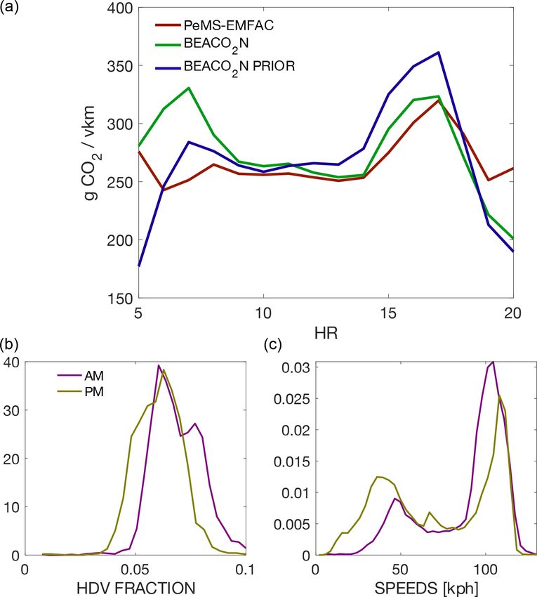
dicted grams of CO2 per vehicle kilometer is small. The We also consider how emission rates compare through-
HDV speed has little impact on the grams of CO2 per vehicle out the day (Fig. 4a). During the evening, PeMS-EMFAC-
kilometer. derived and BEACO2 N-derived emission rates are in good
We use CO2 measurements from 50 BEACO2 N sites agreement. The BEACO2 N grams of CO2 per vehicle kilo-
across the San Francisco Bay Area combined with the meter increases from 256 g CO2 per vehicle kilometer before
BEACO2 N-STILT inversion system to assess highway emis- rush hour (14:00) to 324 g CO2 per vehicle kilometer dur-
sions from our stretch of interest. In Fig. 1, we show the lo- ing peak rush hour (17:00). Likewise, the PeMS-EMFAC-
cation of BEACO2 N sites, the stretch of interest, and emis- derived CO2 per vehicle kilometer increases from 256 to
sion estimates for this stretch. Note that the posterior emis- 320 CO2 per vehicle kilometer over the same time period.
sions move substantially from prior emissions towards what The BEACO2 N prior has a slightly larger increase in the
is estimated from PeMS-EMFAC, particularly during the emission rate over this period (256 g CO2 per vehicle kilo-
evening rush hour, when the prior overestimates emissions meter at 14:00 to 361 g CO2 per vehicle kilometer at 17:00).
by ∼ 20 %. In contrast, during the morning rush hours, we see less
We compare BEACO2 N-derived and PeMS-EMFAC- agreement between PeMS-EMFAC-derived and BEACO2 N-
derived emission rates (grams CO2 per vehicle kilometer) derived emission rate estimates. The BEACO2 N inversion is
and find remarkable agreement. The PeMS-EMFAC-derived similar to the PeMS-EMFAC estimate at 05:00 local time
emission rates range from 225 to 300 g CO2 per vehicle kilo- (280 g CO2 per vehicle kilometer), and the BEACO2N esti-
meter and include the effects of both fleet composition and mate then increases over the morning rush hour to 330 g CO2
variation in speed. For BEACO2 N, we use the total CO2 per vehicle kilometer at 8:00. This behavior is different from
emissions from the inversion at times corresponding to nar- both the BEACO2 N prior (175 g CO2 per vehicle kilometer at
row bins of PeMS-EMFAC (grams of CO2 per vehicle kilo- 05:00 and 275 g CO2 per vehicle kilometer at 08:00) and the
meter). Figure 3a shows an example of data selected at times PeMS-EMFAC calculation which decreases over this period
with PeMS-EMFAC-derived fuel efficiency in the range of (275 g CO2 per vehicle kilometer at 05:00 and 250 g CO2 per
271.4 to 279 g CO2 per vehicle kilometer. There is a range vehicle kilometer at 08:00).
of emissions at each vehicle kilometer because of noise in The discrepancy in the morning between emissions de-
the inversion, variation in speed, and variation in the fleet rived from PeMS-EMFAC and BEACO2 N can potentially be
composition. The slope of a fit to the data in Fig. 3a is an es- reconciled by congestion. There is a nonlinear relationship
timate of the emission rate (Eq. 4), where CO2 emissions are between vehicle speed and the rate of emissions. As such,
defined as hourly emissions summed over BEACO2 N pixels congestion involving nonconstant speeds can result in higher
corresponding to our highway stretch of interest (Fig. 2): emissions than would be estimated using the average vehi-
CO emissons cle speed. This can be seen from a simple example. Consider
2
er g CO2 vkm−1 = . (4) two cases: (1) an LDV traveling at a constant 50 km h−1 for
vkm 1 h and (2) an LDV traveling at 100 km h−1 for 20 min and at
Using 18 months of data for weekdays between 04:00 and 25 km h−1 for 40 min. Both vehicles travel 50 km in 1 h and,
22:00 local time, we compare PeMS-EMFAC-derived and therefore, have the same average speed; however, the emis-
BEACO2 N-derived CO2 per vehicle kilometer (Fig. 3b). sion rate is 461.5 g CO2 per vehicle kilometer at 25 km h−1 ,
These hours were chosen, because they represent the hours 195 g CO2 per vehicle kilometer at 50 km h−1 , and 221 g CO2
for which we expect traffic emissions to be substantially per vehicle kilometer at 100 km h−1 . Using these emission
larger than emissions from other sources in our area of in- rates, the vehicle in the first case would emit 9.75 kg of CO2 ,
terest (see Fig. S3). When fitting to a line forced through
Atmos. Chem. Phys., 22, 3891–3900, 2022 https://doi.org/10.5194/acp-22-3891-2022H. L. Fitzmaurice et al.: Assessing vehicle fuel efficiency using a dense network of CO2 observations 3897
Figure 3. (a) BEACO2 N-derived emissions vs. vehicle kilometers (vkm) for times corresponding to modeled emission rates of 271.4–
279 g CO2 per vehicle kilometer. Red points represent binned medians used in fitting. (b) BEACO2 N-derived vs. PeMS-EMFAC-derived
emission rates with the uncertainty estimate. The black line shows the fit weighted by variance: y = 0.97(.01)x. The gray envelope is the 5 %
deviation from fit, and the red line represents the 1 : 1 line.
whereas the vehicle with the variable speed in the second
case would emit 15 kg of CO2 .
Contrasting the speeds (Fig. 4c) during these two peri-
ods, we see that while both show a bimodal speed distri-
bution, a greater fraction of morning speeds fall into the
40–100 km h−1 range, whereas a greater fraction of evening
speeds are < 40 or > 100 km h−1 . In Fig. S8, we show that
emission rate estimates based on hourly averaged speeds be-
tween 0 and 40 km h−1 and between 100 and 140 km h−1
(more common in evening rush hour) are likely an upper
bound on possible emission rates corresponding to those
hourly averaged speeds, whereas emission rate estimates
based on hourly averaged speeds between 40 and 100 km h−1
(more common in morning rush hour) likely represent a
lower bound of emissions. The predicted range in the emis-
sion rate, resulting from nonconstant speeds combined with
a larger HDV percentage, in the morning (Fig. 4c) is large
enough to explain the mismatch observed during the morn-
ing rush hour.
4 Discussion
The strategic reduction of emissions from transportation is
Figure 4. (a) Emission rates by time of day on weekdays for PeMS-
derived (red), BEACO2N prior (blue), and BEACO2 N posterior
important for both reducing total GHG emissions and im-
(green) data. Probability density functions of the HDV (truck) frac- proving AQ. To make informed decisions that reduce GHGs
tion (b) and speed (c) from a weekday morning (05:00–09:00) and and exposure to poor AQ, policy makers need to know
evening (16:00–20:00) rush hour period on the segment of Interstate (1) how much is being emitted, (2) the location and timing
80 analyzed in Sect. 3. The y axis represents the relative probability of emissions, and (3) the relative impact of various subsector
of the HDV fraction (b) or averaged hourly speed (c). Speeds are processes (e.g., vehicle kilometers and fleet composition).
from individual PeMS sensors, whereas the HDV fraction is aggre- To effectively capture emissions from subsector processes,
gated over the whole stretch under consideration (both directions). models are also reliant on emission factor models, such
as the EMFAC2017 model used in this paper. While our
BEACO2 N-STILT-based estimates largely agree with EM-
https://doi.org/10.5194/acp-22-3891-2022 Atmos. Chem. Phys., 22, 3891–3900, 20223898 H. L. Fitzmaurice et al.: Assessing vehicle fuel efficiency using a dense network of CO2 observations
FAC2017 with respect to CO2 , tracking on-road changes in al. (2019), the impacts of meteorological mismatch during
emission factors will be especially important as the impacts the morning may be offset by a stronger signal, and future
of congestion and fleet composition evolve rapidly, making work should explore the extent to which averaging results
timely updates essential to creating spatially accurate inven- over long time periods or strategic filtering of meteorologi-
tories. For example, the EMFAC model predicts an 18 % de- cal mismatches can combat emission error.
crease in overall CO2 emission rates by 2030, resulting from Beyond further exploration of the elements influencing
the improved fuel efficiency of combustion engine vehicles the sensitivity and precision of the BEACO2 N-STILT sys-
and a transition to hybrid vehicles and EVs (∼ 6.8 % of LDV tem, because each BEACO2 N node measures CO, NOx , and
vehicle kilometers and ∼ 6 % of HDV vehicle kilometers are PM2.5 in addition to CO2 (Kim et al., 2018), the method pre-
expected to be traveled by EVs by 2030). While the increased sented in this paper has the potential to shed light on sub-
share of hybrid vehicles and EVs should work to decrease sector processes impacting the emission factors of these co-
the impact of congestion, a projected increase in total con- emitted species. This is salient because plume-based emis-
gestion and the congested vehicle kilometer share by HDVs sion factor measurements of co-emitted pollutants show that
(Texas A&M Transportation Institute, 2019) is likely to work various emission factor models systematically underestimate
against that trend, making the overall result difficult to pre- emissions (Bishop, 2021), fail to capture spatial heterogene-
dict. ity in these factors due to fleet composition (age and compli-
To our knowledge, this paper represents the first demon- ance with control technologies) for PM (Haugen et al., 2018;
stration that a high-density atmospheric observing network Park, et al., 2016) and black carbon (Preble et al., 2018), or
can both diagnose and quantify the relative contributions of fail to capture the impact of temperature on emission factors.
subsector processes at the neighborhood scale. We demon- Applying these methods across a broader spatial area and
strate that the BEACO2 N network (∼ 2 km spacing) of low- to other species (e.g., PM2.5 , NOx , and CO) should yield in-
cost CO2 sensors can be used to quantify emission rates at a formation of interest to both scientists and policy makers by
specific location (a ∼ 5 km stretch) and by time of day. We
show that, on the highway stretch examined, activity-based 1. revealing spatial and temporal trends in emission rates
emission estimates that account for speed and HDV per- and emission factors across an urban area and quantify-
centage match the inference from atmospheric measurements ing the contributions of congestion, fleet composition,
to within 3 %. Finally, we demonstrate that the BEACO2 N- or other factors to spatial variations;
STILT system detects daily changes in fuel efficiency that 2. identifying and diagnosing the causes of traffic-related
range from 200 to 300 g CO2 per vehicle kilometer and that AQ hot spots that contribute to exposure inequities;
this system would be capable of detecting fleet-wide changes
in fuel efficiency in ∼ 3 years. 3. tracking trends in the above over periods of years to
decades.
5 Outlook
Data availability. The CO2 data used for this study are publicly
available at http://beacon.berkeley.edu (Cohen Research – Univer-
In this work, we have demonstrated that the BEACO2 N-
sity of California Berkeley, 2022). Raw data can be provided upon
STILT system was able to infer emission rates from vehi- request. The traffic data used for this study are publicly available at
cles along a specific stretch of highway. To understand the https://pems.dot.ca.gov/ (California Department of Transportation,
extent to which this method can be applied to other contexts, 2022).
future work should investigate the extent to which various el-
ements of the BEACO2 N-STILT system, including measure-
ment density, error in meteorology used to calculate STILT Supplement. The supplement related to this article is available
trajectories, and the quality of the prior, impact the ability of online at: https://doi.org/10.5194/acp-22-3891-2022-supplement.
similar systems to estimate emissions.
For example, it is possible that the mismatch that we ob-
serve during the morning rush hour may be due to a larger Author contributions. HLF derived the CO2 emissions from
relative meteorological model error in the morning compared traffic data, conceived the idea for the project design, wrote the pa-
with the afternoon and early evening, during which time the per, and collected CO2 data. AJT created and ran the CO2 inversion
boundary layer is relatively well mixed. Because a highly code. HLF, JK, KC, ERD, CN, and PW collected CO2 data. RCC
mixed boundary layer is important for minimizing discrep- gave feedback on the project design and assisted with writing the
paper.
ancies between particle trajectories in the STILT model and
real transport (Lin et al., 2003), inversions typically use only
measurements taken during the afternoon, (Lauvaux et al.,
Competing interests. The contact author has declared that nei-
2016, 2020; Nathan et al., 2019) when the boundary layer ther they nor their co-authors have any competing interests.
is relatively well mixed. However, as discussed by Martin et
Atmos. Chem. Phys., 22, 3891–3900, 2022 https://doi.org/10.5194/acp-22-3891-2022H. L. Fitzmaurice et al.: Assessing vehicle fuel efficiency using a dense network of CO2 observations 3899
Disclaimer. Publisher’s note: Copernicus Publications remains Cohen Research – University of California Berkeley: Berkeley En-
neutral with regard to jurisdictional claims in published maps and vironmental Air-quality & CO2 Network (BEACO2N), http://
institutional affiliations. beacon.berkeley.edu, last access: 15 March 2022.
Davis, S. C., Diegel, S. W., and Boundy, R. G.: Trans-
portation Energy Data Book, Edition 29, Energy, https:
Acknowledgements. The authors are grateful to Kristin Lauter //tedb.ornl.gov/wp-content/uploads/2021/02/TEDB_Ed_39.pdf
and the MSR Urban Innovation group for support with think- (last access: 12 January 2022), 2021.
ing through PeMS data acquisition. This research used the Savio City of Oakland: Oakland Equitable Climate Action
computational cluster resource provided by the Berkeley Research Plan, https://cao-94612.s3.amazonaws.com/documents/
Computing program at UC Berkeley (supported by the UC Berke- Oakland-ECAP-07-24.pdf (last access: 12 January 2022),
ley Chancellor, Vice Chancellor for Research, and Chief Informa- 2020
tion Officer). The authors wish to acknowledge Hannah S. Kenagy Delaria, E. R., Kim, J., Fitzmaurice, H. L., Newman, C.,
for reading through and offering organizational suggestions on the Wooldridge, P. J., Worthington, K., and Cohen, R. C.: The Berke-
manuscript. ley Environmental Air-quality and CO2 Network: field calibra-
tions of sensor temperature dependence and assessment of net-
work scale CO2 accuracy, Atmos. Meas. Tech., 14, 5487–5500,
Financial support. This research has been supported by the NSF, https://doi.org/10.5194/amt-14-5487-2021, 2021.
the Adolph C. and Mary Sprague Miller Institute for Basic Research Gately, C. K. and Hutyra, L. R.: Large Uncertainties in Urban-Scale
in Science, UC Berkeley, and the Koret Foundation. Carbon Emissions, J. Geophys. Res.-Atmos., 122, 11242–11260,
https://doi.org/10.1002/2017JD027359, 2017.
Gately, C. K., Hutyra, L. R., and Wing, I. S.: Cities, traffic, and
CO2 : A multidecadal assessment of trends, drivers, and scal-
Review statement. This paper was edited by Christoph Gerbig
ing relationships. P. Natl. Acad. Sci. USA, 112, 4999–5004,
and reviewed by two anonymous referees.
https://doi.org/10.1073/pnas.1421723112, 2015.
Gately, C. K., Hutyra, L. R., Peterson, S., and Sue Wing, I.: Ur-
ban emissions hotspots: Quantifying vehicle congestion and air
References pollution using mobile phone GPS data, Environ. Pollut., 229,
496–504, https://doi.org/10.1016/j.envpol.2017.05.091, 2017.
Apte, J. S., Messier, K. P., Gani, S., Brauer, M., Kirchstet- Gurney, K. R., Razlivanov, I., Song, Y., Zhou, Y., Benes, B., and
ter, T. W., Lunden, M. M., Marshall, J. D., Portier, C. J., Abdul-Massih, M.: Quantification of fossil fuel CO2 emissions
Vermeulen, R. C. H., and Hamburg, S. P.: High-Resolution on the building/street scale for a large U.S. City, Environ. Sci.
Air Pollution Mapping with Google Street View Cars: Ex- Technol., 46, 12194–12202, https://doi.org/10.1021/es3011282,
ploiting Big Data, Environ. Sci. Technol., 51, 6999–7008. 2012.
https://doi.org/10.1021/acs.est.7b00891, 2017. Gurney, K. R., Liang, J., Roest, G., Song, Y., Mueller, K., and Lau-
Bay Area Air Quality Management District – BAAQMD: Bay vaux, T.: Under-reporting of greenhouse gas emissions in U.S.
Area Emissions Inventory Summary Report Base Year 2011, cities, Nat. Commun., 12, 1–7, https://doi.org/10.1038/s41467-
https://www.baaqmd.gov/~/media/files/planning-and-research/ 020-20871-0, 2021.
emission-inventory/by2011_ghgsummary.pdf (last access: Haugen, M. J. and Bishop, G. A.: Long-Term Fuel-Specific
15 March 2022), 2015. NOx and Particle Emission Trends for In-Use Heavy-Duty Ve-
Bishop, G. A.: Does California’s EMFAC2017 vehicle emis- hicles in California, Environ. Sci. Technol., 52, 6070–6076,
sions model underpredict California light-duty gasoline ve- https://doi.org/10.1021/acs.est.8b00621, 2018.
hicle NOx emissions?, J. Air Waste Ma., 71, 597–606, Kim, J., Shusterman, A. A., Lieschke, K. J., Newman, C.,
https://doi.org/10.1080/10962247.2020.1869121, 2021. and Cohen, R. C.: The BErkeley Atmospheric CO2 Ob-
Boswell, M. R. and Madilyn Jacobson, A. R.: 2019 Report on servation Network: field calibration and evaluation of low-
the State of Climate Action Plans in California, https://ww2. cost air quality sensors, Atmos. Meas. Tech., 11, 1937–1946,
arb.ca.gov/sites/default/files/2020-03/17RD033.pdf (last access: https://doi.org/10.5194/amt-11-1937-2018, 2018.
12 January 2022), 2019. Kim, J. Turner, A. J., Fitzmaurice, H. L., Delaria, E. R., Newman,
California Air Resources Board: PROGRESS REPORT: Cal- C., Wooldridge, P. J., and Cohen, R. C.: Observing annual trends
ifornia’s Sustainable Communities and Climate Protection in vehicular CO2 emissions, Environ. Sci. Technol., in review,
Act, (November), 96, https://ww2.arb.ca.gov/sites/default/files/ 2021.
2018-11/Final2018Report_SB150_112618_02_Report.pdf (last Kwon, J., Varaiya, P., and Skabardonis, A. Estimation of Truck
access: 12 January 2022), 2018. Traffic Volume from Single Loop Detectors with Lane-to-
California Department of Transportation: Performance Measure- Lane Speed Correlation, Transp. Res. Rec., 684, 106–117,
ment System, California Department of Transportation [data set], https://doi.org/10.3141/1856-11, 2003.
https://pems.dot.ca.gov, last access: 15 March 2022. Lauvaux, T., Miles, N. L., Deng, A., Richardson, S. J., Cambal-
Caubel, J. J., Cados, T. E., Preble, C. V., and Kirchstet- iza, M. O., Davis, K. J., Gaudet, B. Gurney, K. R., Huang, J.
ter, T. W.: A Distributed Network of 100 Black Carbon O’Keefe, D., Song, Y., Karion, A., Oda, T., Patarsuk, R., Ra-
Sensors for 100 Days of Air Quality Monitoring in West zlivanov, I., Sarmiento, D., Shepson, P, Sweeney, C. Turnbull,
Oakland, California, Environ. Sci. Technol., 53, 7564–7573, J., and Wu, K.: High-resolution atmospheric inversion of urban
https://doi.org/10.1021/acs.est.9b00282, 2019.
https://doi.org/10.5194/acp-22-3891-2022 Atmos. Chem. Phys., 22, 3891–3900, 20223900 H. L. Fitzmaurice et al.: Assessing vehicle fuel efficiency using a dense network of CO2 observations CO2 emissions during the dormant season of the Indianapolis Seto K. C., Dhakal, S., Bigio, A., Blanco, H., Delgado, G. C., De- flux experiment (INFLUX), J. Geophys. Res., 121, 5213–5236, war, D., Huang, L., Inaba, A., Kansal, A., Lwasa, S., McMa- https://doi.org/10.1002/2015JD024473, 2016. hon, J. E., Müller, D. B., Murakami, J., Nagendra, H., and Lauvaux, T., Gurney, K. R., Miles, N. L., Davis, K. J., Richard- Ramaswami, A.: Human Settlements, Infrastructure and Spa- son, S. J., Deng, A., Nathan, B. J., Oda, T. Wang, J. A., tial Planning. In: Climate Change 2014: Mitigation of Climate Hutyra, L., and Turnbull, J.: Policy-relevant assessment of ur- Change. Contribution of Working Group III to the Fifth Assess- ban CO2 emissions, Environ. Sci. Technol., 54, 10237–10245, ment Report of the Intergovernmental Panel on Climate Change, https://doi.org/10.1021/acs.est.0c00343, 2020. edited by: Edenhofer, O., Pichs-Madruga, R., Sokona, Y., Fara- Lin, J. C., Gerbig, C., Wofsy, S. C., Andrews, A. E., Daube, hani, E., Kadner, S., Seyboth, K., Adler, A., Baum, I., Brun- B. C., Davis, K. J., and Grainger, C. A.: A near-field tool ner, S., Eickemeier, P., Kriemann, B., Savolainen, J., Schlömer, for simulating the upstream influence of atmospheric ob- S., von Stechow, C., Zwickel, T., and Minx, J. C., Cam- servations: The Stochastic Time-Inverted Lagrangian Trans- bridge University Press, Cambridge, United Kingdom and New port (STILT) model, J. Geophys. Res.-Atmos., 108, 4493, York, NY, USA, https://www.ipcc.ch/site/assets/uploads/2018/ https://doi.org/10.1029/2002JD003161, 2003. 02/ipcc_wg3_ar5_chapter12.pdf (last access: 18 March 2022), Martin, C. R., Zeng, N., Karion, A., Mueller, K., Ghosh, S., Lopez- 2014. Coto, I., Gurney, K. R., Oda, T., Prasad, K., Liu, Y., and Dicker- Shusterman, A. A., Teige, V. E., Turner, A. J., Newman, C., Kim, J., son, R.R., Investigating sources of variability and error in simula- and Cohen, R. C.: The BErkeley Atmospheric CO2 Observation tions of carbon dioxide in an urban region, Atmos. Environ., 199, Network: initial evaluation, Atmos. Chem. Phys., 16, 13449– 55–69, https://doi.org/10.1016/j.atmosenv.2018.11.013, 2019. 13463, https://doi.org/10.5194/acp-16-13449-2016, 2016. McDonald, B. C., McBride, Z. C., Martin, E. W., and Harley, Tessum, C. W., Paolella, D. A., Chambliss, S. E., Apte, J. S., Hill, J. R. A.: High-resolution mapping of motor vehicle carbon diox- D., and Marshall, J. D.: PM2.5 polluters disproportionately and ide emissions, J. Geophys. Res.-Atmos., 119, 5283–5298, systemically affect people of color in the United States, Science https://doi.org/10.1002/2013JD021219, 2014. Advances, 7, 1–7, https://doi.org/10.1126/sciadv.abf4491, 2021. Moua, F.: California Annual Fuel Outlet Report Results (CEC- Texas A&M Transportation Institute: Urban Mobility Report 2019, A15), Energy Assessments Division, California Energy Comis- 182, https://static.tti.tamu.edu/tti.tamu.edu/documents/umr/ sion, https://www.energy.ca.gov/media/3874 (last access: 13 Jan- archive/mobility-report-2019.pdf (last access: 13 January 2022), uary 2022), 2020. 2019. Nathan, B. J., Lauvaux, T., Turnbull, J. C., Richardson, S. Turner, A. J., Shusterman, A. A., McDonald, B. C., Teige, V., J., Miles, N. L. and Gurney, K. R., Source sector attribu- Harley, R. A., and Cohen, R. C.: Network design for quantify- tion of CO2 emissions using an urban CO / CO2 Bayesian ing urban CO2 emissions: assessing trade-offs between precision inversion system, J. Geophys. Res.-Atmos., 123, 13–611, and network density, Atmos. Chem. Phys., 16, 13465–13475, https://doi.org/10.1029/2018JD029231, 2018. https://doi.org/10.5194/acp-16-13465-2016, 2016. Newman, S., Xu, X., Gurney, K. R., Hsu, Y. K., Li, K. F., Jiang, Turner, A. J., Kim, J., Fitzmaurice, H., Newman, C., Wor- X., Keeling, R., Feng, S., O’Keefe, D., Patarasuk, R., Wong, K. thington, K., Chan, K., Wooldridge, P. J., Köehler, P., W., Rao, P., Fischer, M. L., and Yung, Y. L.: Toward consis- Frankenberg, C., and Cohen, R. C.: Observed impacts tency between trends in bottom-up CO2 emissions and top-down of COVID-19 on urban CO2 Emissions, Geophys. Res. atmospheric measurements in the Los Angeles megacity, At- Lett., 47, p.e2020GL090037, Geophys. Res. Lett., 47, 1–6, mos. Chem. Phys., 16, 3843–3863, https://doi.org/10.5194/acp- https://doi.org/10.1029/2020GL090037, 2020a. 16-3843-2016, 2016. Turner, A. J., Köhler, P., Magney, T. S., Frankenberg, C., Fung, I., Park, S. S., Vijayan, A., Mara, S. L., and Herner, J. and Cohen, R. C.: A double peak in the seasonality of Califor- D.: Investigating the real-world emission characteristics of nia’s photosynthesis as observed from space, Biogeosciences, 17, light-duty gasoline vehicles and their relationship to lo- 405–422, https://doi.org/10.5194/bg-17-405-2020, 2020b. cal socioeconomic conditions in three communities in Los Angeles, California, J. Air Waste Ma., 66, 1031–1044, https://doi.org/10.1080/10962247.2016.1197166, 2016. Preble, C. V., Cados, T. E., Harley, R. A., and Kirchstetter, T. W.: In-Use Performance and Durability of Particle Filters on Heavy- Duty Diesel Trucks, Environ. Sci. Technol., 52, 11913–11921, https://doi.org/10.1021/acs.est.8b02977, 2018. Atmos. Chem. Phys., 22, 3891–3900, 2022 https://doi.org/10.5194/acp-22-3891-2022
You can also read