A Study on Distortion Estimation Based on Image Gradients
←
→
Page content transcription
If your browser does not render page correctly, please read the page content below
sensors
Article
A Study on Distortion Estimation Based on Image Gradients
Sin Chee Chin             , Chee-Onn Chow * , Jeevan Kanesan                    and Joon Huang Chuah

                                          Department of Electrical Engineering, Faculty of Engineering, Universiti Malaya, Kuala Lumpur 50603, Malaysia;
                                          imsinchee@gmail.com (S.C.C.); jievan@um.edu.my (J.K.); jhchuah@um.edu.my (J.H.C.)
                                          * Correspondence: cochow@um.edu.my

                                          Abstract: Image noise is a variation of uneven pixel values that occurs randomly. A good estimation
                                          of image noise parameters is crucial in image noise modeling, image denoising, and image quality
                                          assessment. To the best of our knowledge, there is no single estimator that can predict all noise
                                          parameters for multiple noise types. The first contribution of our research was to design a noise
                                          data feature extractor that can effectively extract noise information from the image pair. The second
                                          contribution of our work leveraged other noise parameter estimation algorithms that can only predict
                                          one type of noise. Our proposed method, DE-G, can estimate additive noise, multiplicative noise, and
                                          impulsive noise from single-source images accurately. We also show the capability of the proposed
                                          method in estimating multiple corruptions.

                                          Keywords: noise; distortion estimation; multiple corruption estimation; image gradients

                                          1. Introduction

                                         Image noise is one of the major sources of corruption of an image. Severe noise
Citation: Chin, S.C.; Chow, C.-O.;        in an image can cause information loss. Image noises are described as the incorrect bit
Kanesan, J.; Chuah, J.H. A Study on       information on the image due to several reasons, for example a false bit-flip is caused by
Distortion Estimation Based on            the thermal noise in the internal circuitry of the camera, and random noises are due to the
Image Gradients. Sensors 2022, 22,        random exposure of the light sensor in the camera to radiation when taking a photo. The
639. https://doi.org/10.3390/
                                          nature and strength of noise have a high correlation with the surrounding environment.
s22020639
                                          A good noise type and strength estimator is needed to study the relationship between
Academic Editors: Ying-Ren Chien,         the surrounding environment and the resultant image we received. For example, X-ray
Mu Zhou, Liang-Hung Wang and              projection suffers from severe noise corruption and noise distribution, commonly modeled
Xun Zhang                                 as Poisson noise or Rician noise. The standard deviation of noise has a high correlation
                                          with the X-ray voltage and current because reducing the power of the X-ray will cause the
Received: 17 December 2021
                                          Bremsstrahlung curve to change [1].
Accepted: 12 January 2022
Published: 14 January 2022
                                                Throughout the years, several noise models have been proposed to model the noise
                                          observed in a noisy image. Additive White Gaussian Noise (AWGN) is commonly used as
Publisher’s Note: MDPI stays neutral      the random noise in both one-dimensional signal and image noise. Salt-and-pepper noise
with regard to jurisdictional claims in   is proposed as the false bit-flip effect shown in images when there is thermal noise present.
published maps and institutional affil-
                                          Noise modeling is extremely important as the noise model’s parameter can be used as a
iations.
                                          reference for the nature of the noise observed in the image. Image Quality Assessment (IQA)
                                          is a systematic way of grading the image noise corruption level by comparing the score
                                          predicted by the algorithm and the Mean Opinion Score (MOS) of several subjects ranging
Copyright: © 2022 by the authors.
                                          from experts to novices. IQA is designed to accommodate all types of distortions and give
Licensee MDPI, Basel, Switzerland.
                                          an overall score. It is hard to judge the noise strength and severity of the corruption of
This article is an open access article    the image from the predicted score of IQA because there might be more than one type of
distributed under the terms and           distortion present in the noisy image and the correlation between the IQA score across
conditions of the Creative Commons        different types of noise is different. As image noise is randomly distributed with a specific
Attribution (CC BY) license (https://     distribution, the IQA score is often non-reproducible. A noise model parameter estimation
creativecommons.org/licenses/by/          is a good representation of the nature of noise. Hence, an inverse process is required to
4.0/).                                    estimate the noise parameters.

Sensors 2022, 22, 639. https://doi.org/10.3390/s22020639                                                      https://www.mdpi.com/journal/sensors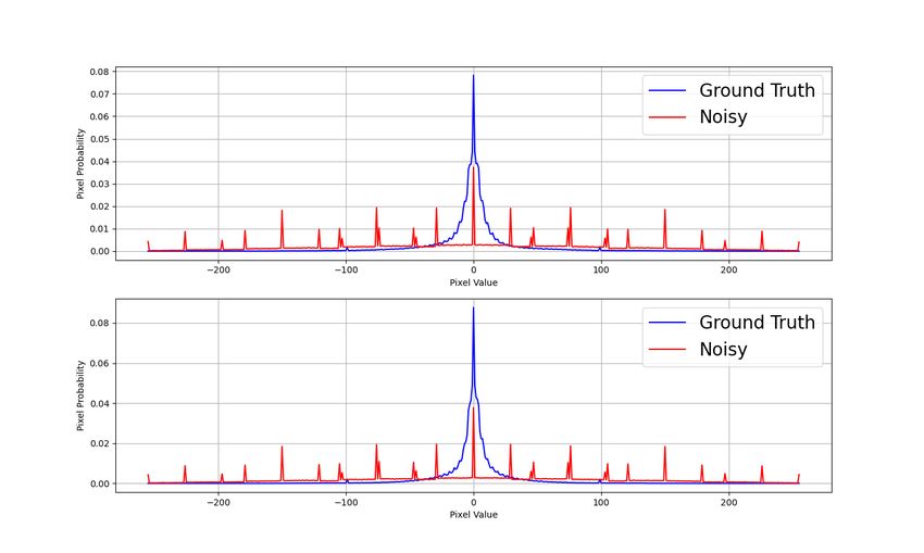
Sensors 2022, 22, 639                                                                                             2 of 22

                              A picture is worth a thousand words. An image can describe the environment perfectly
                        without the need for description and explanation. Feature extraction is a technique to
                        extract information from the input signal. Feature extraction can downsample the input
                        signal by extracting information that we need for further processing. Recent developments
                        in machine learning have explored different architectures for performing deep feature
                        extraction in tasks such as classification, object detection, and anomaly detection [2–5]. With
                        the emergence of 5G technology, the boom in the volume of data has made the deep learning
                        approach feasible because machine learning requires an abundance of data to perform
                        the fine-tuning of the millions of parameters in the neural network. Developments in
                        image recovery such as U-net and Hi-Net have taken a supervised approach in performing
                        image manipulation, such as denoising, deblurring, etc. [6,7]. The architecture of these
                        autoencoder networks downsample the vector space and upsample it again to produce
                        images that are free of noise. Recently, the extension of U-net’s capability to performing
                        denoising in medical images has been studied. To train such a network, the ground
                        truth–noisy pair must be known. Unfortunately, such an image dataset is very hard to
                        achieve due to reasons such as privacy issues and health issues. Besides from medical
                        images, other types of ground truth–noisy image pairs that are hard to collect are motion
                        blur and glare. Deblur GAN, which is designed to perform motion deblurring of motion
                        blur images through an adversarial training approach, requires an image pair to conduct
                        training [8,9]. Motion blur images are hard to obtain because the experiments are hard to
                        replicate, especially on natural images.
                              A recent study showed the possibility of using synthetic data to generate the ground
                        truth–noisy image pair by using a simulator that closely resembles the actual environ-
                        ment [10]. Reference [11] obtained the image pair of glare images and performed glare
                        removal. The result showed significant improvement because more data were used for
                        training. Data acquisition in a simulated environment is less costly and versatile compared
                        to real-life data collection. A well-designed simulator allows the user to change the res-
                        olution, physical limits, and noise of the acquired data. The data obtained are no longer
                        restricted to the physical limitations such as being unable to place two cameras at the same
                        spot while taking a photo at different shutter speeds (data acquisition of the motion blur
                        image) and a virtual environment allowing data collection all day long. The process of data
                        collection does not require human supervision in a simulated environment. However, the
                        data obtained from a virtual environment cannot be used as the training dataset for any
                        machine learning application because noise is absent from the acquired dataset. The correct
                        noise injection is applied to the synthetic data obtained through the simulator. Augmented
                        data with noise injection need to be similar to the actual noise seen in real-life training data.
                              Besides creating realistic synthetic data and studying the environment, noise strength
                        estimation is also important in noise suppression. Image denoising is a heavily studied
                        field in quality image acquisition. The goal of image denoising is to preserve the spatial
                        domain and to suppress the range domain. Some prior information of the range domain
                        is needed such as the Standard Deviation (STD) of the range domain to perform image
                        denoising. These parameters are commonly known as the denoising strength. The greater
                        the denoising strength, the stronger the denoising effect is. Extreme denoising strength will
                        cause the spatial domain to be suppressed. An adequate guess of the standard deviation
                        of the image noise is needed to perform denoising to prevent spatial domain information
                        from being removed. Recent developments in image denoising involve machine learning
                        approaches such as U-net, but the downside for such an approach is the data-driven image
                        recovery and the amount of data required. Classical denoising algorithms such as Block
                        Matching 3D (BM3D) and total variation denoising require prior information input as the
                        parameter for denoising [12,13]. Noise strength estimation is important as we can use this
                        method to perform a correlation study for the type of noise, the strength of the noise, and
                        the suitable parameter to be used for the image denoising algorithm.
                              In this paper, we propose Distortion Estimation using the image Gradient (DE-G).
                        We performed feature extraction from the noisy image by comparing the feature space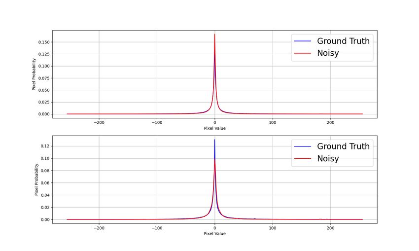
Sensors 2022, 22, 639                                                                                          3 of 22

                        with the ground truth–noisy image pair. In this research, we show that DE-G can esti-
                        mate the noise strength of any given noise model accurately. We categorized noise as
                        additive and multiplicative noise and conducted noise parameter estimation using DE-G
                        to estimate the parameters of the noise model. Next, we further extended our work to
                        estimating multiple distortions and showed the capability of our proposed method to
                        estimate combined distortion.
                             The remainder of this paper is organized as follows. Section 2 gives the literature
                        review. Section 3 explains the need for noise parameter estimation and the proposed
                        method (DE-G) in detail. Section 4 presents the results and discussions. Section 5 gives the
                        conclusion and the usage of DE-G.

                        2. Literature Review
                              Noise is a major source of corruption in images. A noisy image can cause information
                        loss. Noises can be classified into two major classes: additive noise and multiplicative
                        noise. Additive noises are noises that are added to the image such as Gaussian noise.
                        Multiplicative noise is multiplied with the ground truth image such as speckle noise [14].
                        Other distortions such as blurring are modeled by taking the convolution of the point spread
                        function with the ground truth image [15]. The point spread function is a 2-dimensional
                        array describing the radiation intensity distribution in the image of a point source [15].
                              We name these corruptions as noise and distortion respectively in this paper. Ref-
                        erence [14] discussed noise models such as Gaussian noise, salt-and-pepper noise, and
                        grain noise. Reference [16] updated some noise models that have been added throughout
                        the years and provided a quick review of the noise models. Reference [17] proposed a
                        Monte Carlo simulation approach for rendering these film grain noises using a Poisson
                        distribution and other algorithms.
                              X-rays are commonly used in medical images such as Magnetic Resonance Imaging
                        (MRI) and Advance X-ray Imaging (AXI) for silicon defect detection. X-ray doses are
                        desired to be as low as possible to reduce harm towards the subject, but as the dose
                        decreases, the X-ray noise increases. These noises are known as quantum noise and are
                        often modeled with Poisson noise [18]. Electronics’ noises were described by [19] as false
                        bit-flips due to thermal heating in electronics. Salt-and-pepper noise is used to model these
                        false bit-flips [20]. Reference [20] also presented a way to perform a median filter at the
                        circuit level to remove such noise in an image.

                        2.1. Noise Parameter Estimation
                             Noise can be mathematically modeled, and its strength is dependent on the input
                        parameters, for example random noise that is modeled using a Gaussian distribution. As
                        the standard deviation of the Gaussian noise model increases, the image will suffer from a
                        noisier corruption. Noise parameter estimation estimates these noises accurately at a high
                        repeatability. Noise parameter estimation is important for the correct noise modeling of the
                        image such that the latent noisy image is not overly noisy and close to reality.
                             Reference [21] proposed a noise estimation method by using Bayesian MAP inferencing
                        on a distorted image and performed a review on noise modeling in a CCD camera. The
                        authors proposed that noises that are seen from the images are mostly from the propagation
                        stage. Noise can be irradiance-dependent or independent noise. These noises are additive
                        and passed through a Camera Response Function (CRF). The authors ignored the additive
                        noise that is added to the image after the image passes through the CRF as they claimed
                        that with modern-day cameras, additive noise that affects the image is very small. One
                        of the most widely used methods for estimating noise is through the Mean Absolute
                        Deviation (MAD). However, this method is commonly used in local and smooth kernels.
                        Reference [22] decomposed an image into the wavelet components and trained with a set of
                        13 images. Reference [22] used wavelet transform as a feature extractor from the degraded
                        image and used these features to fit a final output value. However, the model can only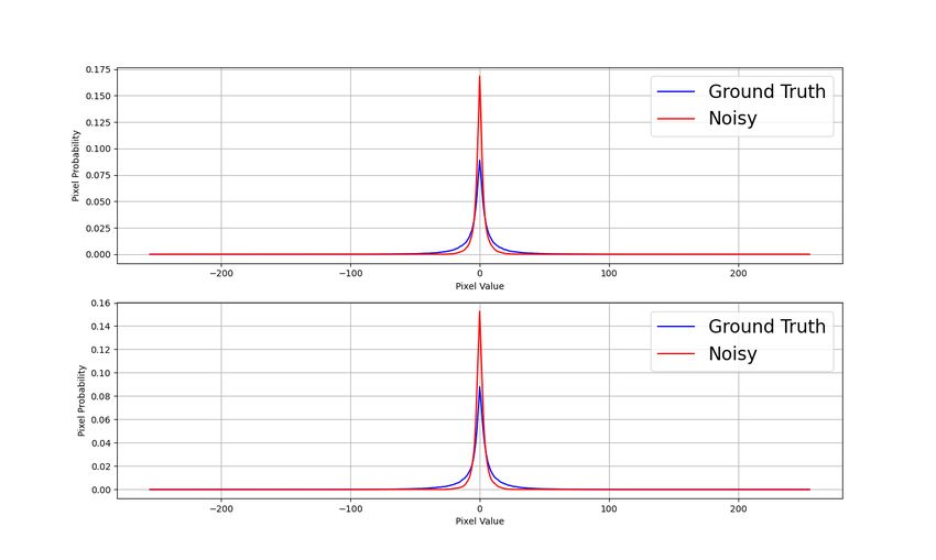
Sensors 2022, 22, 639                                                                                          4 of 22

                        predict noise parameters that are in the training dataset and is not as versatile asother
                        noise models.
                             The median absolute deviation counters the idea of the mean absolute deviation
                        in estimating noise [23]. The median absolute deviation is more robust than the mean
                        absolute deviation and is less affected by outliers, which makes the edges in non-smooth
                        regions less affected by the overall score. Reference [24] challenged the median absolute
                        deviation method and proposed the Residual Autocorrelation Power (RAP). The RAP can
                        estimate the additive noise standard deviation to a high level of accuracy when compared
                        with the median absolute deviation. Reference [25] suggested that the noise estimation of
                        colored images and grayscale images is different as colored images have multiple channels
                        to take under consideration, while grayscale images, which are commonly used in the
                        medical field, have a single channel. Reference [26] used a multivariate Gaussian noise
                        model to visualize the pixel spread of each channel and estimate the covariance of noise by
                        comparing each channel. Through an iterative process, the noise covariance was estimated.
                        Reference [27] used the mean deviation at a certain Region Of Interest (ROI) and computed
                        the estimated standard deviation of the Gaussian noise added to the image. The result
                        showed high consistency and accuracy at low-level noise (σ = 5), but started to deviate at
                        higher noise levels (σ = 10, σ = 15). Reference [28] performed a blind quality assessment
                        using the method of moments to measure the signal-to-noise ratio of the one-dimensional
                        signal of a cosine waveform. Reference [29] used a statistics-based approach for noise
                        estimation using the skewness of the image pair and estimated the strength of the noise of
                        the Additive White Gaussian Noise (AWGN). Reference [30] performed noise estimation
                        on mammograms by using Rician noise modeling and used the estimated value to perform
                        image denoising using a nonlocal mean denoising filter.
                             Noise study and strength estimation have been given much attention because noise
                        allows researchers to have a better understanding of the environment that causes noise and
                        the effect of fine-tuning these physical parameters’ relationship on the image quality. Much
                        work has been performed in noise estimation working on specific noises such as X-ray
                        noise, described by different distributions, and general noise, modeled using Gaussian
                        noise. The ability of these methods to predict other forms of noise has not been discussed
                        formally, and their capability of estimating combined noise has also not been explored.

                        2.2. Usage of Parameter Estimation
                              An accurate prediction of the noise level from the image allows for less human inter-
                        vention in performing image processing and environment physics study. Classical image
                        denoising algorithms are widely used in performing image recovery. Image denoising
                        requires some prior information from the user to perform image denoising. The Gaussian
                        low-pass filter is one of the most well-known filters that removes high-frequency noise from
                        the image, but the structural integrity of the image will be sacrificed when the denoising
                        strength is too strong. An improved version of the Gaussian filter is the bilateral filter,
                        which takes a spatial standard deviation and a range standard deviation. The bilateral filter
                        is a nonlinear and edge-preserving denoising algorithm, but the denoising strength must
                        be set correctly or it will approximate the Gaussian blur [31]. The adaptive Wiener filter
                        and the Modified Median Wiener Filter (MMWF) perform denoising by taking the noise
                        variance of the image [32,33]. BM3D requires the user to input a standard deviation that
                        directly relates to the noise level of the image [12]. These denoising algorithms are very
                        popular in the medical imaging chain. The input parameters of the denoising algorithm
                        have a high correlation with the noise model parameters. Another image processing al-
                        gorithm that needs the noise information is image segmentation. Reference [34] used a
                        fuzzy C-means clustering algorithm to perform image segmentation on images that were
                        corrupted by impulsive noise. The method can be further improved by providing the
                        algorithm with the noise information. Hence, noise information is crucial in performing
                        image processing algorithms.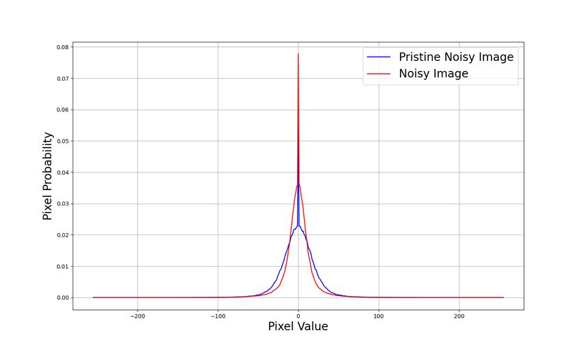
Sensors 2022, 22, 639                                                                                            5 of 22

                             The root cause of noise can be due to the physics of the surrounding environment or
                        during the conversion of photons to pixel values in the camera. Conventionally, brighter
                        pixels are due to more photons received by the camera sensor during the shot duration. The
                        camera setting can significantly affect the image quality, for example increasing the shutter
                        speed will reduce the exposure time. Noise will become more apparent compared to the
                        overall signal received. The overall Signal-to-Noise Ratio (SNR) [35] will decrease with
                        increasing exposure time. Light travels differently at different frequencies. High-frequency
                        light will be able to penetrate opaque objects and allow us to see through the object. A
                        well-known example of the real-life usage of these properties is in defect detection using
                        X-rays in AXI. The X-ray projection noise is caused by the scattering of X-ray photons when
                        they pass through an object. The scattering angle is dependent on the energy of the X-rays
                        (frequency) and the type of material being used as the X-ray source [36]. Hence, the study
                        of the noise model parameter can be of great help in determining the noise level of the X-ray
                        projection image and selecting an optimal standard deviation for the denoising algorithm
                        without the need for human intervention.

                        2.3. Image Quality Assessment
                              The image gradient gives more insight into the physical structure of an image by
                        showing the edges of an image using filters such as the Sobel, Prewitt, and Laplace filter.
                        This gives rise to the idea that the image gradient can be used to measure the image quality.
                        For example, blurred images have less edge information than clear images. Reference [37]
                        proposed image quality assessment using gradient similarity, which utilizes the image
                        gradient to compute an overall score from the luminance, contrast, and structure. Refer-
                        ence [38] proposed the Gradient Magnitude Standard Deviation (GMSD), which calculates
                        the standard deviation from the quality map of a gradient of the image. Structural Similarity
                        Index Measure (SSIM) compares the ground truth image with the restored image with three
                        metrics, luminance, contrast, and structural similarity; all three metrics are consolidated
                        into one overall score [39]. The Multi-scale SSIM (MS-SSIM) extends the idea of the SSIM
                        and changes the final consolidation score formula to obtain a more accurate grading [40].
                        Information-Weighted SSIM (IW-SSIM) also extends the SSIM by adding a weighted pool-
                        ing to the SSIM [41]. These image quality assessments show a high correlation with the
                        mean opinion score of humans. However, the type and strength of distortion of the image
                        is not specifically estimated.
                              The Laplacian of Gaussian (LoG) and the Difference of Gaussian (DoG) pass the
                        images through a Gaussian blur, effectively removing noise in the image and comparing
                        the structural difference between the reference image and the filtered image [42]. Recent
                        advancements include using visual saliency, chrominance, and gradient magnitude to grade
                        an image in CIELAB, as proposed by [43]. Reference [44] proposed the SuperPixel-based
                        SIMilarity Index (SPSIM), which obtains a set of image pixels that have the same visual
                        characteristics, and called them superpixels. Each superpixel is graded with the superpixel
                        luminance similarity, superpixel chrominance, and gradient similarity.
                              The Human Visual System (HVS) is extremely complex at perceiving information
                        from the real world and transmitting the scenario that we see in our daily lives to our
                        brain for processing. Image quality assessment grading is performed by comparing the
                        objective scores of the subjects (participants in the experiment) and the given score of the
                        image quality assessment. The free-energy principle would suggest that when a human
                        sees a corrupted image, he/she will have a mental picture of how clean the image should
                        look [45]. By comparing the mental picture and the given corrupted image, humans can
                        give a score to the corrupted image. The Mean Opinion Score (MOS) and Difference Mean
                        Opinion Score (DMOS) are two common metrics computed with the result obtained from
                        the human subjective experiment [46]. To mimic the complex HVS, visual saliency is used
                        to put more emphasis on the foreground of the image, rather than the background of the
                        image. Reference [47] proposed using deep neural networks for both no-reference and
                        full-reference image quality assessment. Before the pooling layer arrives at the final score, a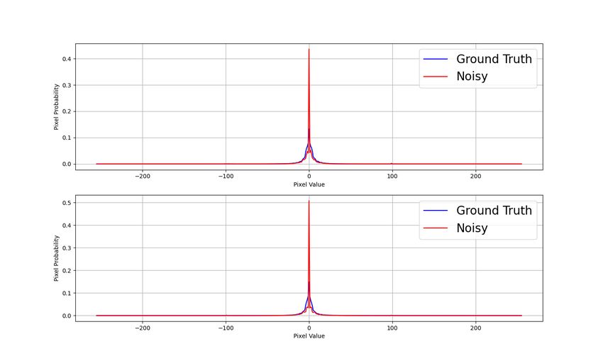
Sensors 2022, 22, 639 6 of 22
fully connected neural network is used to estimate the weights of each patch. Reference [48]
proposed using an attention residual network for full-reference image quality prediction,
which maps out the saliency for final grading.
We classify these image quality assessments into two different types of distortion:
(i) noise and (ii) structural difference. Noise includes all types of noise, Gaussian noise,
Poisson noise, etc, and structural distortion includes Gaussian blur, compression distortion,
etc. Image quality assessment is considered as an overall score for the noisy image, and the
score is obtained through the combination of the information retained, feature similarity,
etc. Image quality assessment can be used as a guide for designing a good feature extractor.
Image quality assessment that is based on the image gradient exhibits a good response
towards noise such as in the GMSD. The noisier the noisy image is, the greater the GMSD
score. Hence, we used the image gradient as a method of feature extraction for estimating
the noise parameters.
3. Methodology
We compared the commonly used Image Quality Assessment (IQA) with the predicted
value to observe the linearity and performance of IQA in estimating the image score for
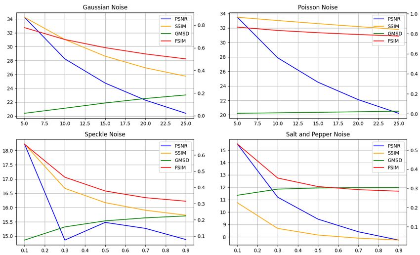
different noise types. Table 1 shows the simulated result of different IQAs with different
noise models. The experiment was conducted using the Kodak image dataset. We compared
the linearity using the Peak-Signal-to-Noise Ratio (PSNR), Structural Similarity (SSIM),
Gradient Magnitude Standard Deviation (GMSD), and Feature Similarity (FSIM). The
numerical value of the IQA score reflects the severity of the corruption of the noise model.
Gaussian noise shows a good linearity performance between the IQA scores and the
strength of the noise. However, the other noise model does not have the same linearity
performance as Gaussian noise. In Poisson noise, the PSNR still shows a good description
of the noise strength, but other IQA scores are not as sensitive as the PSNR. Speckle noise
and salt-and-pepper noise have a much lower PSNR value compared to Gaussian and
Poisson noise, and the PSNR curve is damped faster. The GMSD of both speckle and
salt-and-pepper noise saturate very fast compared to Gaussian and Poisson noise. The plot
of Table 1 is shown in Figure 1. This shows that IQA gives a good overall score of the image
and is able to aid in predicting Gaussian noise. However, the performance of IQA in noise
prediction is not recommended.
Table 1. Image quality assessment of different noise types.
Noise Type Truth PSNR SSIM GMSD FSIM
Gaussian 5 34.24 0.8699 0.0213 0.7781
10 28.24 0.6732 0.0662 0.6734
15 24.75 0.5258 0.1124 0.6011
20 22.28 0.4228 0.1520 0.5457
25 20.39 0.3489 0.1834 0.5018
Poisson 5 33.48 0.9644 0.0047 0.8659
10 27.88 0.9318 0.0095 0.8325
15 24.51 0.9007 0.0146 0.8100
20 22.10 0.8710 0.0200 0.7919
25 20.22 0.8424 0.0257 0.7768
Speckle 0.1 18.23 0.6682 0.0744 0.6672
0.3 14.86 0.3943 0.1557 0.4631
0.5 15.48 0.3061 0.1932 0.3780
0.7 15.27 0.2589 0.2118 0.3367
0.9 14.88 0.2283 0.2237 0.3148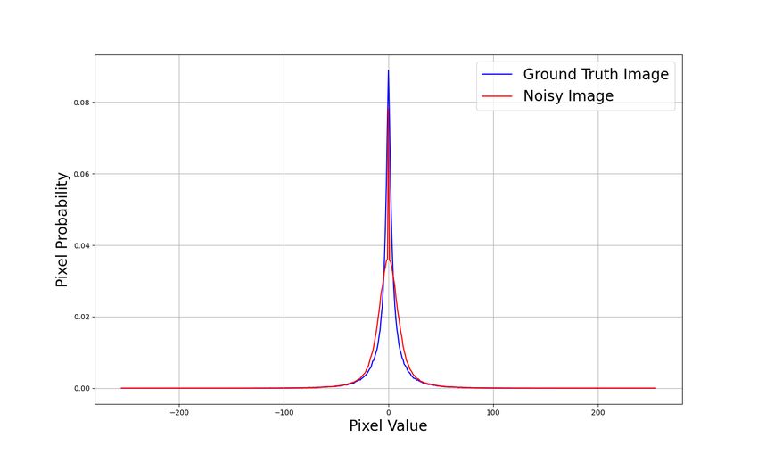
Sensors 2022, 22, 639                                                                                          7 of 22

                        Table 1. Cont.

                          Noise Type         Truth           PSNR            SSIM          GMSD           FSIM
                            Salt-and-
                                              0.1            15.49           0.2250        0.2642        0.5319
                             Pepper
                                              0.3            11.20           0.0908        0.2963        0.3542
                                              0.5            9.43            0.0564        0.3023        0.3096
                                              0.7            8.41            0.0399        0.3035        0.2935
                                              0.9            7.74            0.0300        0.3038        0.2855

                        Figure 1. Comparison of IQA with respect to the noise parameter.

                        3.1. Noise Estimation Modeling
                              All image quality assessment methods of scoring are the consolidation of different
                        types of distortions applied to an image. We aimed to create an algorithm that extracts
                        the distortion information effectively from the noisy image statistically. DE-G provides
                        the information of the dominant and secondary distortions in the resulting image. The
                        proposed method is not restricted to the size of the image and can account for any known
                        distortion that can be described through mathematical modeling. Besides, the proposed
                        method can also account for multiple combined distortions.
                              Reference [49] showed that natural images exhibit a generalized Gaussian curve when
                        taking the pixel count of the derivative of the image. Reference [49] used this property to
                        perform image deblurring by curve fitting using the K number of the Gaussian distribution,
                        while [50] used a piecewise function to model the image gradient property of natural
                        images. This property inspired us to observe image information in a statistical viewpoint,
                        and we observed that different noises will result in different image gradient responses.
                        Instead of sacrificing the accuracy, we adopted a full-reference approach, which requires
                        the input of a ground truth image to be used as a reference.
                              Distortion models usually have one or more parameters to set the distortion properties.
                        Gaussian noise consists of two parameters, the mean and the standard deviation. The mean
                        sets the luminance of the noise, while the standard deviation describes the probability of
                        the pixel spread. A higher standard deviation in Gaussian noise results in a noisier image.
                        The mean of Gaussian noise is set to zero as the luminance is normally unchanged when
                        the image is corrupted by noise. Image blurring is modeled with Gaussian blur, and it takes
                        one parameter, which is the kernel size of the blur function. The larger the kernel size, the
                        more severe the blurring effect is. Noisy images are described as shown in Equation (1),
                        where the image we received is f and the noise is n.
Sensors 2022, 22, 639 8 of 22
f = g+n (1)
Another type of distortion that might occur during the imaging chain process is at the
CRF where the camera is out of focus or experiences motion blur. These distortions have a
convolutional relationship between the ground truth image and the CRF. Assuming that
noise is temporal, n is additive after the convolution. Hence, we modeled the equation for
the received image as shown in Equation (2):
f = h∗g+n (2)
where h is the CRF and n is the additive noise. Note that noise can be additive or mul-
tiplicative, but here, we describe the mathematical modeling of a distorted image in an
additive manner. We then took the derivative of the image and plotted the pixel spread
from −255 to 255. The details of the image gradient formulation are shown in Appendix A.
The derivative of an image is obtained by using Equations (3) and (4):
Ix (i, j) = I (i + 1, j) − I (i, j) (3)
Iy (i, j) = I (i, j + 1) − I (i, j) (4)
where i, j ∈ W + 1, H + 1. W and H are the width and height of the image. Ix and Iy are
zero padded at the left end and bottom end of the image, respectively. Ix is the resultant
partial derivative map across the width, and Iy is the resultant partial derivative map across
the height. Note that the partial derivative is computed separately and shown separately
as there are cases where we can detect noise on the X-axis or the Y-axis.
3.2. Image Gradient Response
Noise strength is hard to estimate through human judgment. Figure 2a is the ground
truth image and Figure 2b is the noisy image with Gaussian noise of zero mean and
standard deviation of five, respectively. The image gradient statistics response in the x
direction is shown in Figure 2c. The blue curve represents the ground truth image, while
the red curve represents the distorted image.
Then, we conducted a study to estimate the standard deviation of Gaussian noise
using the image gradient. A ground truth image was first injected with Gaussian noise
with a known standard deviation. We call this a pristine noisy image. We then injected
noise into the same ground truth image with a guessed standard deviation. We call this the
latent noisy image. The latent noisy image as shown in Figure 3a has a standard deviation
of 5, while the pristine noisy image has a standard deviation of 10 (Figure 3b). The image
gradient statistics is shown in Figure 3c. The comparison of the pristine noisy image of
standard deviation 10 and the latent noise image of standard deviation 5 shows that the
greater the standard deviation of the noise model is, the greater the suppression in 0. By
increasing the guessed standard deviation closer to 10, the two curves will become closer to
each other. When the curve fit each other, the standard deviation of the latent noisy image
is the same as the pristine noisy image.Sensors 2022, 22, 639 9 of 22
(a)
(c)
(b)
Figure 2. Ground truth–noisy image pair with their respective image gradient statistics. The image
gradient statistics are very close to each other, which are similar to the original image, but the features
are clearly described through the image gradient statistics. (a) Ground truth image. (b) Noisy image.
(c) Image gradient statistics along the X-axis.
(a)
(c)
(b)
Figure 3. Comparison of image gradient statistics of the pristine noisy image and latent noisy image.
The pristine noisy image has a standard deviation of 10, while the latent noisy image has a standard
deviation of 5. (a) Latent distorted image, standard deviation of 5. (b) Pristine distorted image,
standard deviation of 10. (c) Image gradient statistics along the X-axis.Sensors 2022, 22, 639 10 of 22
To evaluate the image gradient response of the algorithm, we used an open-source
dataset to validate our claim. The LIVE dataset consists of ground truth–noisy image pairs
where the noisy images were created using 5 different distortions [39,46,46]:
1. JPEG compressed images;
2. JPEG2000 compressed images;
3. Gaussian blur;
4. White noise;
5. Fast-fading Rayleigh channel.
For each of the distortions, we observed a different image gradient response. Figure 4a–e
shows the example of the degradation for each image corruption from the LIVE dataset.
The ground truth image of each responding noisy image is from Figure 4f–j. Gaussian blur
and the fast-fading Rayleigh channel showed a very similar distortion as they significantly
reduced the image frequency. This is the reason why this caused the gradient statistics to
tighten at a higher frequency. JPEG compressed images have blurring at some regions,
but also, the frequency of the image increases around the blurred region. This is observed
from the vegetation in the background of the dancer and added artifacts on the stairs.
JPEG2000-compressed images pixels are highly pixelated from the compression, and
this will cause the image gradient to be reduced. However, the overall image is still
maintained, and this causes the image to have a tight neck at a relatively lower frequency,
but not at a higher frequency. This is in contrast to Gaussian blur and the fast-fading
Rayleigh channel, which remove the high-frequency elements from the image. White
noise consists of random noise having the properties of a Gaussian distribution. The
image is corrupted with severe white noise, which causes the gradient distribution to be
flattened. The center still maintains the sharpest peak, as there is still some information
remaining in the image.
From Figure 5a–e, the noise-corrupted images are JPEG2000-compressed images,
JPEG-compressed images, Gaussian blur, white noise, and the fast-fading Rayleigh channel.
The upper graph shows the image gradient statistics of the horizontal gradient, while
the bottom graph shows the image gradient statistics of the vertical gradient. The blur
line is the ground truth image, and the red line is a noisy image. JPEG2000-compressed
images tighten the lower neck of the distribution, but the rest of the distribution remains
relatively unchanged. JPEG-compressed images have the response of widening the neck
of the distribution, but lower near 0. White noise consists of random spikes in the noisy
image distribution, and we noticed that the distribution is not only symmetric, but the
gradient distribution in X is similar in Y, despite the difference in the X and Y distribution
of the original image. Gaussian blur is very similar to JPEG compression and is tightened
in the lower upper neck, but the gradient near 0 remains relatively unchanged. Only the
large gradient difference is affected. The fast-fading Rayleigh channel shows a significant
shift from the high gradient difference to the low gradient difference. The neck of the
distribution is significantly tightened, and the tip is lifted.Sensors 2022, 22, 639 11 of 22
(a) (b) (c) (d) (e)
(f) (g) (h) (i) (j)
Figure 4. Corruption from the LIVE dataset. The corruption is performed on the entire image. The
cropped noisy and ground truth pair image is shown in (a–j). The noisy image is in (a,b), while (f–j)
is the respective ground truth image. The noisy images consist of (a) JPEG2000 compression, (b) JPEG
compression, (c) white noise, (d) Gaussian blur, and (e) the fast-fading Rayleigh channel.
In order to quantify the amount of loss between two curves, a cost function is needed
to measure the Area Under the Curve (AUC) of the blue (ground truth) and red (noisy)
curve. The greater the area, the greater the loss of the latent noisy image is. The loss function
we chose to use was the Canberra distance. The Canberra distance is the measurement of
the distance between the two curves. The formula for the Canberra distance is shown in
Equation (5). The Canberra distance was chosen because it provides a bounded value from
0 to 1 for each extracted feature.
| xn − xt |
d= ∑ | xn | + | xt | (5)
where d is the Canberra distance, xn is the noisy image, and xt is the ground truth image.
The overall algorithm for DE-G is as shown in Algorithm 1. The first step is taking in
a pristine noisy image, T, and a latent noisy image, X. Then, the size of the image is
determined. Both images are passed to the feature extractor through the image gradient
and return four image gradient distributions:
1. Image Gradient with respect to x of the pristine image, δx ( T );
2. Image Gradient with respect to y of the pristine image, δy ( T );
3. Image Gradient with respect to x of the latent image, δx ( X );
4. Image Gradient with respect to y of the latent image, δy ( X ).Sensors 2022, 22, 639 12 of 22
(a) (b)
(c) (d)
(e)
Figure 5. Image gradient distribution for each type of distortion in the LIVE dataset. The up-
per graph is the image gradient in x, while the lower graph is the image gradient in y. Cases:
(a) JPEG2000 compression, (b) JPEG compression, (c) white noise, (d) Gaussian blur, and (e) fast-
fading Rayleigh channel.
3.3. Noise Type Response Using the Proposed Feature Vectors
Since the image gradient pixels range from −255 to 255, the total feature vectors at
the X and Y axis is 1022. Using a clean image (Lena), we augmented the clean image
with several noise models. The noise models included additive noise (Gaussian noise and
Poisson noise), multiplicative noise (speckle noise), and impulse noise (salt-and-pepper
noise). Gaussian noise was set to a fixed mean value and a variable standard deviation.
Poisson noise took exactly one input to manipulate the noise spread, which was the variance.Sensors 2022, 22, 639 13 of 22
We altered the speckle noise by adding a weighting coefficient to the speckle noise, as
shown in Equation (6):
f = g + g × N (0, 1) × w (6)
where w is the weightage that controls the speckle noise strength. The salt-and-pepper noise
has two parameters, which are the ratio of salt-to-pepper and the number of events of false
bit-flips. Using the proposed feature extractor, we observed the image gradient response
of the three types of noise models discussed above. The clean image was corrupted with
Gaussian noise (Figure 6a), speckle noise (Figure 6b), and salt-and-pepper noise (Figure 6c).
Figure 7a is the image gradient response of Figure 6a. Figure 7b is the image gradient
response of Figure 6b. Figure 7c is the image gradient response of Figure 6c.
(a)
(b) (c)
Figure 6. Noisy image corrupted with Gaussian noise (a), speckle noise (b), and salt-and-pepper
noise (c). It is hard to differentiate speckle noise from salt-and-pepper noise by the human eye.
3.4. Noise Strength Prediction
To estimate the noise strength, the Canberra distance was used as a loss function by
taking the sum of the distance between δx ( T ), δx ( X ) and δy ( T ), δy ( X ) to obtain ∆ x and ∆y ,
respectively. The L2 of ∆ x and ∆y was taken as the final loss function. For colored image,
the L p of ∆ x and ∆y was taken, where p depends on the subpixel channel. The overall
algorithm for DE-G is shown in Algorithm 1. Our proposed method requires several pieces
of a priori knowledge such as the ground truth image, the noisy image, and the noise
model. The optimum noise parameters are estimated through each iteration.Sensors 2022, 22, 639 14 of 22
(a) Image Gradient of Gaussian Noise (b) Image Gradient of Speckle Noise
(c) Image Gradient of Salt-and-Pepper Noise
Figure 7. Image gradient response. (a) is the image gradient of Figure 6a (red) compared to the clean
image (blue). (b) is the image gradient of Figure 6b (red) compared to the clean image (blue). (c) is
the image gradient of Figure 6c (red) compared to the clean image (blue). Note that the extracted
features clearly differentiate each noise type.
Algorithm 1 Algorithm for the loss function to estimate the noise level.
INPUT (X, T)
W, H ← shape( X )
δx ( T ) ← T (i + 1, j) − T (i, j) for i, j ∈ W, H
δy ( T ) ← T (i, j + 1) − T (i, j) for i, j ∈ W, H
δx ( X ) ← X (i + 1, j) − X (i, j) for i, j ∈ W, H
δy ( X ) ← X (i, j + 1) − X (i, j) for i, j ∈ W, H
|δx ( Xi ) − δx ( Ti )|
∆x ← ∑ for i = −255, . . . , 255
|δx ( Xi )| + |δx ( Ti )|
|δy ( Xi ) − δy ( Ti )|
∆y ← ∑ for i = −255, . . . , 255
|δy ( Xi )| + |δy ( Ti )|
loss ← L2 (∆ x , ∆y )
return loss
We used the Kodak image dataset to perform the evaluation of the estimated noise
parameters. We classified the conducted test into four types of distortion estimations:
additive noise estimation, multiplicative noise estimation, impulsive noise estimation, and
combined noise estimation. The Kodak images consist of natural images that have a size
of 768 × 512 or 512 × 768. We resized the images to 192 × 128 or 128 × 192 depending on
the original image size. We used Particle Swarm Optimization (PSO) to estimate the noise
parameters. To prevent heavy oscillation, we adopted a batch mean strategy by taking the
mean loss of 20 noisy image batches. The overall algorithm is shown in Figure 8. In real-life
usage, the pristine noisy image is the noisy image in the ground truth–noisy image pair
instead of noise injection into the clean image.Sensors 2022, 22, 639 15 of 22
Figure 8. Block diagram for noise parameter estimation. The clean image is the ground truth image.
To demonstrate the capability of DE-G in estimating accurate noise parameters, the clean image is
injected with noise with a known set of parameters to produce the pristine noise image. The clean
image is then injected with noise with a set of guessed parameters. The pristine noisy image and the
latent noisy image are compared using DE-G. Through each iteration, the guessed parameters are
updated using Particle Swarm Optimization (PSO). The algorithm ends after the maximum iteration
number of PSO is reached.
4. Results and Discussions
The experiment was conducted by injecting noise with a known parameter and at-
tempting to estimate the injected noise parameter. The parameter of the intended noisy
image is referred to as the ground truth parameter, and the noisy image is known as the
pristine noisy image. The predicted parameter is known as the estimated parameter, and
the predicted noisy image is known as the latent noisy image. The mean and the standard
deviation of the ground truth parameter and the predicted parameter were calculated. We
also evaluated the Mean-Squared Error (MSE), Mean Absolute Deviation (MAD), and the
error percentage between the predicted value from DE-G and the known ground truth
(Mean Relative Error Rate (MRER)). We also compared the accuracy of the Canberra dis-
tance with the KL divergence for all four scenarios. The KL divergence is a commonly used
loss function to quantify the difference between two probability distributions [51].
4.1. Parameter Estimation of Additive Noise
Additive noise describes that noise that has an additive nature in the image. The
additive nature of noise means that noise is independent of the image pixel value. Gaussian
noise is the most-often found noise in images. Random noise in images might be caused by
the surrounding radiation, random processes in the camera, or random error in the image.
The mean of Gaussian noise is commonly set to zero because noise does not have a DC
component to offset the pixel value of noise. We conducted the estimation of Gaussian
noise with a mean of 0 and a standard deviation of 5, 10, 15, and 20. The results are shown
in Table 2. Our proposed method was compared with [29] in predicting the standard
deviation of Gaussian noise. The method of [29] does not show the capability of predicting
other noise models. In the next subsection, we show the ability of DE-G in predicting other
noise models such as multiplicative noise, impulsive noise, and combined noise.Sensors 2022, 22, 639 16 of 22
Table 2. Gaussian noise standard deviation estimation. The mean is set to zero, and the strength of
the Gaussian noise is determined by the standard deviation.
DE-G with Canberra DE-G with KL
σt Heng et al. [29]
Distance Divergence
5 4.97 5.03 4.84
10 10.03 9.97 9.65
15 15.09 14.94 14.60
20 20.03 20.12 19.45
MSE 0.0050 0.0049 0.1536
MAD 0.058 0.06 0.3666
MRER 2% 6% 4%
4.2. Parameter Estimation of Multiplicative Noise
An example of multiplicative noise is speckle noise. Speckle noise strength is depen-
dent on the pixel value. Speckle noise follows the normal distribution:
X ∼ N (µ, σ2 ) (7)
Comparing Equations (6) and (7), we obtain µ = g and σ2 = w × g. The mean and the
variance of the normal distribution are related to the original ground truth image. Speckle
noise is commonly found in radar and medical ultrasound images. It is caused by the
coherent processing of back-scattered signals from multiple distributed targets. DE-G can
predict the weighting factor, w, of speckle noise, and the results are shown in Table 3.
Table 3. Speckle noise weight estimation. The strength of distortion is determined by the weight of
the speckle noise model as shown in Equation (6).
DE-G with Canberra
w DE-G with KL Divergence
Distance
0.3 0.2945 0.2742
0.5 0.5055 0.4737
0.7 0.6961 0.6990
MSE 0.00002 0.00045
MAD 0.0050 0.0177
MRER 1% 5%
4.3. Parameter Estimation of Impulsive Noise
Salt-and-pepper noise is noise caused by thermal noise in electronics. Energy is lost in
electronic components as heat energy. As heat energy is not efficiently ventilated, the heat
energy will cause a high temperature in the circuit. The high temperature of the circuit will
cause the bit value to malfunction and result in false bit-flips. The false bit-flips will result in
random pixels in the image to be white (salt) or black (pepper). Salt-and-pepper noise will
significantly change in the tail of the image gradient response. The salt-and-pepper noise
is modeled with two parameter inputs, the ratio between salt-and-pepper, ranging from
(0, 1), and the ratio of defect pixel to the total amount of pixels in the image. In this study,
the ratio of salt-and-pepper was varied from 0.2 to 0.7 and the amount of salt-and-pepper
was predicted. The results are shown in Table 4.Sensors 2022, 22, 639 17 of 22
Table 4. Salt-and-pepper noise parameter estimation.
DE-G with Canberra DE-G with KL
Ratio Amount
Distance Divergence
0.2 0.3 0.3157 0.2854
0.2 0.5 0.5303 0.4914
0.2 0.7 0.6774 0.7288
0.5 0.3 0.3075 0.2963
0.5 0.5 0.5046 0.4946
0.5 0.7 0.6925 0.7034
0.7 0.3 0.3048 0.2955
0.7 0.5 0.5068 0.4997
0.7 0.7 0.6879 0.6970
MSE 0.0002 0.0001
MAE 0.0120 0.0080
MRER 3% 3%
4.4. Parameter Estimation of Combined Corruption
Realistic images consist of several distortions applied to the image. As described in
Equation (2), the received image can consist of a convolutional distortion and noise. We
used Gaussian blur and Gaussian noise as our distortion combination. Gaussian blur is
commonly found in images when the image is out of focus. The recovery process requires
a known window size to perform the inverse process. Gaussian blur is not considered as
noise that is added to the clean image, but a convolutional distortion. Gaussian blur had
one parameter, which is the blur window size. The larger the window size, the greater
the blur strength. We denote the window size as W and the standard deviation of the
Gaussian noise as σ. The true window size and standard deviation have a subscript of
t. In Sections 4.1–4.4, parameter estimation was performed using the Canberra distance
and Kullback–Leibler divergence. The Canberra distance was chosen for the parameter
estimation for combined noise because of the stability of the Canberra distance in predicting
noise. The results are shown in Table 5. The predicted parameters in Table 5 are the mean
of the predicted parameters in the Kodak dataset.
Table 5. Combined noise parameters’ estimation.
DE-G with Canberra
True Parameter
Distance
Wt σt W σ
5 5 5.2917 4.9411
5 10 4.7083 9.6002
10 5 11.2500 5.1347
10 10 10.6667 7.5610
MSE 0.5443 1.5325
MAD 0.6250 0.7581
MRER 7% 10%
4.5. Discussions
In this section, we discuss the results we obtained through our experiment in esti-
mating the noise strength. The Canberra distance was used for DE-G in predicting noise
parameters and showed a stable and accurate result. Our method is not restricted by image
size, nor the noise type. We were able to predict the Gaussian noise standard deviation with
a lower MSE than [29], but with a higher error rate of 6% for the Canberra distance and 4%
for the KL divergence. However, we leveraged this issue through the capability of DE-G in
predicting other noise models using a unified algorithm. DE-G can predict speckle noise
and salt-and-pepper noise with an error rate of less than 3% for the Canberra distance andSensors 2022, 22, 639 18 of 22
5% for the KL divergence. Due to this reason, we chose the Canberra distance as the loss
function for the combined corruption parameters’ estimation. We showed the capability of
DE-G in estimating the noise parameters for Gaussian blur and Gaussian noise with error
rates of 7% and 10%, respectively.
Previous work focused on a specific type of noise, and the approaches were through
looking at the power spectrum, frequency domain, and statistical viewpoint. Such methods
restrict the algorithm to predict only one type of noise. DE-G is able to predict different
noise types and combined corruption, which proves to be useful and highly desirable, as
real-life images consist of more than one noise source.
As shown in Sections 4.1–4.4, we showed the capability of DE-G in estimating noise
parameters of different noise models. Our method is not restricted to any noise model and
is able to predict multiple parameters as the output for any known noise model. Instead
of having a correlated SNR or aggregated score such as in IQA, we would argue that our
method is very useful for researchers to study the nature of noise. This is because with the
prior knowledge of the noise model, our method can neglect the other distortions applied
to the image. This is important because real-life imaging systems consist of more than one
type of noise present.
The proposed method comes with several restrictions, the requirement of the the
ground truth–noisy image pair and the prior knowledge of the noise type. Some ground
truth–noisy image pair are hard to obtain due to the limitations of the process of data
collection. Data acquisition has become an expensive and tedious task for researchers.
Our proposed method will aid in the process of data collection by performing realistic
data augmentation with accurate noise model parameters. The process of data acquisition
can be minimized after the user has obtained a confident noise model parameter using
DE-G. The ground truth image can also be obtained through image processing techniques
without losing any information such as image averaging [52]. DE-G can be used to study
the expected noise model parameters. Synthetic noisy images that mimic real–life images
can be obtained by injecting noise into the averaged image. Next, noise models are often
well-established, and our proposed method can also be used in researching new noise
models by proving the loss.
5. Conclusions
Images are becoming one of the useful forms of information transfer between the
real world and the digital world. However, the corruption by noise is one of the major
threats that reduces image quality. The proposed method, DE-G, effectively extracts noise
information from the image pair by employing the Canberra distance as the loss function.
DE-G is able to predict Gaussian noise (additive) with an MRER of 6%, speckle noise
(multiplicative) with an MRER of 1%, and salt-and-pepper noise (impulsive) with an MRER
of 3%. DE-G is also able to perform combined corruption (Gaussian blur and Gaussian
noise) parameters’ estimation with an MRER of 7% and 10%, respectively.
Our work proposed a multi-noise parameter estimation for different noise types, and
it is also capable of estimating combined corruption. We proposed a feature extractor that
effectively extracts noise information from the ground truth–noisy image pair. This will be
useful because our method accounts for any image size. We also proposed a loss function
that can estimate the optimum noise parameters from the extracted features.
The nature of noise has a strong relationship with the surrounding environment. Noise
strength will change with the settings of the surrounding environment. The most effective
way to reduce and prevent noise in an image is to understand the nature of the noises and
suppress them by changing the parameters of the surroundings. Noise model parameters
can be used as a guide for a specific type of noise. Since the strength of synthetic noise
is highly dependent on the noise model parameters, an accurate estimation of the noise
model is highly desirable to study the relationship between the physical environment and
the noise model parameter. Besides the study of the nature of noise, noise modeling is
also very important in image augmentation. Contrastive loss has recently gained muchSensors 2022, 22, 639 19 of 22
attention from the machine learning community. One of the major parts of contrastive
learning is data augmentation. However, the way data are augmented is not specified. We
argue that noise augmentation will help in the training process, but the correct range of
noise model parameters should be defined clearly according to the application and the
physical environment. Ground truth–noisy image pairs are hard to obtain due to several
restrictions. A good understanding of the nature of noise and the noise strength is needed
to create synthetic data for training purposes. As the number of data increase, the training
process can be more robust.
The next step in our research is to address the weakness of DE-G, which is the need
for a ground truth image by balancing the accuracy and applicability. References [49,50]
showed that natural images exhibit a generalized Gaussian distribution trend and used
that property to perform image deblurring. Using a similar approach, we can design a no-
reference noise parameters’ estimation algorithm. In Section 3.3, we presented the features’
behavior under different types of noise. Noise-type prediction can also be performed
through a machine learning approach. Classical deep learning requires a fixed input to the
model, and our feature extraction technique can fix any image size to a fixed size input
feature. Next, we will also look into the possibility of using DE-G in performing image
quality assessment. We will also aim to improve the parameter estimation algorithm by
using a more robust approach such as [53]. Further development of DE-G in the study
of the environment, data augmentation, and data generation will be carried out to aid in
better algorithm design and the ever-growing machine learning data acquisition.
Author Contributions: Conceptualization, S.C.C. and C.-O.C.; methodology, S.C.C.; software, S.C.C.;
validation, S.C.C. and J.K.; formal analysis, S.C.C. and J.K.; investigation, S.C.C.; resources, S.C.C.;
data curation, S.C.C.; writing—original draft preparation, S.C.C.; writing—review and editing, S.C.C.
and C.-O.C.; visualization, S.C.C. and C.-O.C.; supervision, C.-O.C., J.K., and J.H.C.; project admin-
istration, C.-O.C.; funding acquisition, C.-O.C. All authors have read and agreed to the published
version of the manuscript.
Funding: This research was funded by the Impact Oriented Interdisciplinary Research Grant (IIRG)
Programme, University of Malaya (IIRG002B-19IISS).
Institutional Review Board Statement: Not applicable.
Informed Consent Statement: Not applicable.
Data Availability Statement: Restrictions apply to the availability of these data. Data was obtained
from Laboratory for Image & Video Engineering at the University of Texas at Austin and are available
from the authors with the permission of University of Texas at Austin.
Conflicts of Interest: The authors declare no conflict of interest.
Appendix A. Image Gradient Formulation
A corrupted image can be described as shown in (A1):
f = h∗g+n (A1)
where f is the corrupted image, h is the camera response function, g is the ground truth
image, and n is noise. The image gradient is taken as the first derivative of f as follows,
f 0 = g0 ∗ h + n0 (A2)
Next, a difference operator, D, is needed to measure the distance between f 0 and
g0 effectively. An example of D ( f 0 , g0 ) is taking the difference between f 0 and g0 . The
information from h and n is not removed, but g0 is also present in f 0 − g0 , as shown below.
f 0 − g 0 = g 0 ∗ ( h − 1) + n 0 (A3)Sensors 2022, 22, 639 20 of 22
To effectively remove g0 from D ( f 0 , g0 ), we consider f 0 and g0 as a probability mass function,
N( f 0)
P1 ( X = f 0 ) = (A4)
W×H
N ( g0 )
P2 ( X = g0 ) = (A5)
W×H
The probability mass function calculates the probability of a given value occurring
in the entire image of width W and height H. This will effectively restrict the feature size
because the limit of the image is known. For example, for grayscale images, the image
gradient ranges from −255 to 255, which has a feature space of 511. This will hold true given
any image size. DE-G uses the Canberra distance as the difference operator to estimate the
optimum noise parameter.
| P ( X = f 0 ) − P2 ( X = g0 )|
D ( f 0 , g0 ) = ∑ | P11(X = f 0 )| + | P2 ( X = g0 )|
(A6)
The greater the Canberra distance, the noisier it will be. We extended this idea to
estimate the noise strength through minimizing the cost function between the pristine noisy
image (the noisy image) and the latent noisy image (the ground truth image injected with
the noise of an known parameter). The flowchart of the entire process of noise strength
estimation is shown in Figure 8. The program was written with Python 3.7. Note that
D ( f 0 , g0 ) has two directions, x and y. Dx is denoted as the image gradient in the x direction,
while Dy is denoted as the image gradient in the y direction. According to Algorithm 1, Dx
is ∆ x and Dy is ∆y , respectively. The final loss function is L2 for both the x and y direction.
For colored images, L2 is taken for each channel.
References
1. Huda, W.; Abrahams, R.B. Radiographic techniques, contrast, and noise in X-ray imaging. Am. J. Roentgenol. 2015, 204,
W126–W131. [CrossRef] [PubMed]
2. He, K.; Zhang, X.; Ren, S.; Sun, J. Deep residual learning for image recognition. In Proceedings of the IEEE Conference on
Computer Vision and Pattern Recognition, Las Vegas, NV, USA, 27–30 June 2016; pp. 770–778.
3. Iandola, F.; Moskewicz, M.; Karayev, S.; Girshick, R.; Darrell, T.; Keutzer, K. Densenet: Implementing efficient convnet descriptor
pyramids. arXiv 2014, arXiv:1404.1869.
4. Dosovitskiy, A.; Beyer, L.; Kolesnikov, A.; Weissenborn, D.; Zhai, X.; Unterthiner, T.; Dehghani, M.; Minderer, M.; Heigold, G.;
Gelly, S.; et al. An image is worth 16 × 16 words: Transformers for image recognition at scale. arXiv 2020, arXiv:2010.11929.
5. Touvron, H.; Bojanowski, P.; Caron, M.; Cord, M.; El-Nouby, A.; Grave, E.; Izacard, G.; Joulin, A.; Synnaeve, G.; Verbeek, J.; et al.
Resmlp: Feedforward networks for image classification with data-efficient training. arXiv 2021, arXiv:2105.03404.
6. Tripathi, M. Facial image denoising using AutoEncoder and UNET. Herit. Sustain. Dev. 2021, 3, 89–96. [CrossRef]
7. Chen, L.; Lu, X.; Zhang, J.; Chu, X.; Chen, C. HINet: Half Instance Normalization Network for Image Restoration. In Proceedings
of the IEEE/CVF Conference on Computer Vision and Pattern Recognition (CVPR) Workshops, Nashville, TN, USA, 19–25 June
2021; pp. 182–192.
8. Kupyn, O.; Budzan, V.; Mykhailych, M.; Mishkin, D.; Matas, J. DeblurGAN: Blind Motion Deblurring Using Conditional
Adversarial Networks. arXiv 2017, arXiv:1711.07064.
9. Kupyn, O.; Martyniuk, T.; Wu, J.; Wang, Z. DeblurGAN-v2: Deblurring (Orders-of-Magnitude) Faster and Better. In Proceedings
of the IEEE International Conference on Computer Vision (ICCV), Seoul, Korea, 27–28 October 2019.
10. Fabbri, M.; Brasó, G.; Maugeri, G.; Cetintas, O.; Gasparini, R.; Osep, A.; Calderara, S.; Leal-Taixe, L.; Cucchiara, R. MOTSynth:
How Can Synthetic Data Help Pedestrian Detection and Tracking? In Proceedings of the IEEE/CVF International Conference on
Computer Vision, Online, 11–17 October 2021; pp. 10849–10859.
11. Nikolenko, S.I. Synthetic Simulated Environments. In Synthetic Data for Deep Learning; Springer: Berlin/Heidelberg, Germany,
2021; pp. 195–215.
12. Lebrun, M. An analysis and implementation of the BM3D image denoising method. Image Process. Online 2012, 2012, 175–213.
[CrossRef]
13. Chambolle, A. An algorithm for total variation minimization and applications. J. Math. Imaging Vis. 2004, 20, 89–97.
14. Boncelet, C. Image noise models. In The Essential Guide to Image Processing; Elsevier: Amsterdam, The Netherlands, 2009;
pp. 143–167.You can also read