A seasonal algorithm of the snow-covered area fraction for mountainous terrain
←
→
Page content transcription
If your browser does not render page correctly, please read the page content below

The Cryosphere, 15, 4607–4624, 2021
https://doi.org/10.5194/tc-15-4607-2021
© Author(s) 2021. This work is distributed under
the Creative Commons Attribution 4.0 License.

A seasonal algorithm of the snow-covered area fraction
for mountainous terrain
Nora Helbig1 , Michael Schirmer1 , Jan Magnusson2 , Flavia Mäder1,3 , Alec van Herwijnen1 , Louis Quéno1 ,
Yves Bühler1 , Jeff S. Deems4 , and Simon Gascoin5
1 WSL    Institute for Snow and Avalanche Research SLF, Davos, Switzerland
2 Statkraft AS, Oslo, Norway
3 Institute of Geography, University of Bern, Bern, Switzerland
4 National Snow and Ice Data Center, University of Colorado, Boulder, CO, USA
5 Centre d’Etudes Spatiales de la Biosphère, CESBIO, Univ. Toulouse, CNES/CNRS/INRAE/IRD/UPS,

31401 Toulouse, France

Correspondence: Nora Helbig (norahelbig@gmail.com)

Received: 22 December 2020 – Discussion started: 5 January 2021
Revised: 13 August 2021 – Accepted: 2 September 2021 – Published: 29 September 2021

Abstract. The snow cover spatial variability in moun-            1   Introduction
tainous terrain changes considerably over the course of a
snow season. In this context, fractional snow-covered area       In mountainous terrain, the large spatial variability in the
(fSCA) is an essential model parameter characterizing how        snow cover is driven by the interaction of meteorological
much ground surface in a grid cell is currently covered by       variables with the underlying topography. Over the course
snow. We present a seasonal fSCA algorithm using a re-           of a winter season, the dominating topographic interac-
cent scale-independent fSCA parameterization. For the sea-       tions with wind, precipitation and radiation vary consider-
sonal implementation, we track snow depth (HS) and snow          ably, generating characteristic seasonal dynamics of spatial
water equivalent (SWE) and account for several alternat-         snow depth variability (e.g., Luce et al., 1999). This spatial
ing accumulation–ablation phases. Besides tracking HS and        variability, or how much of the ground is actually covered
SWE, the seasonal fSCA algorithm only requires subgrid           by snow, is typically characterized by the fractional snow-
terrain parameters from a fine-scale summer digital eleva-       covered area (fSCA). The fSCA is a crucial parameter in
tion model. We implemented the new algorithm in a multi-         model applications such as weather forecasts (e.g., Douville
layer energy balance snow cover model. To evaluate the spa-      et al., 1995; Doms et al., 2011), hydrological modeling (e.g.,
tiotemporal changes in modeled fSCA, we compiled three           Luce et al., 1999; Thirel et al., 2013; Magnusson et al., 2014;
independent fSCA data sets derived from airborne-acquired        Griessinger et al., 2016, 2019) and avalanche forecasting
fine-scale HS data and from satellite and terrestrial imagery.   (Bellaire and Jamieson, 2013; Horton and Jamieson, 2016;
Overall, modeled daily 1 km fSCA values had normalized           Vionnet et al., 2014), and it is also used for climate scenarios
root mean square errors of 7 %, 12 % and 21 % for the three      (e.g., Roesch et al., 2001; Mudryk et al., 2020).
data sets, and some seasonal trends were identified. Com-           The fSCA can be retrieved from various satellite sensor
paring our algorithm performances to the performances of         images, including Moderate Resolution Imaging Spectrora-
the CLM5.0 fSCA algorithm implemented in the multilayer          diometer (MODIS) or Sentinel-2 (e.g., Hall et al., 1995;
snow cover model demonstrated that our full seasonal fSCA        Painter et al., 2009; Drusch et al., 2012; Masson et al., 2018;
algorithm better represented seasonal trends. Overall, the re-   Gascoin et al., 2019). Nevertheless, solutions are required
sults suggest that our seasonal fSCA algorithm can be ap-        to correct for temporally and spatially inconsistent coverage
plied in other geographic regions by any snow model appli-       due to time gaps between satellite revisits, data delivery and
cation.                                                          the frequent presence of clouds (Parajka and Blöschl, 2006;
                                                                 Gascoin et al., 2015). Though fine-scale spatial snow cover

Published by Copernicus Publications on behalf of the European Geosciences Union.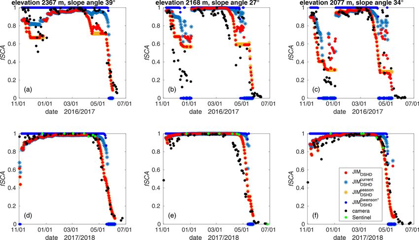
4608                    N. Helbig et al.: A seasonal algorithm of the snow-covered area fraction for mountainous terrain

models provide spatial snow depth distributions that could         model implementation of a closed form fSCA parameteriza-
be used to derive coarse-scale fSCA, applying such models          tion also needs to account for alternating snow accumulation
to larger regions is generally not feasible. This is in part due   and melt events during the season. Especially at lower ele-
to computational cost, a lack of detailed input data and limi-     vations and increasingly so with climate change, the separa-
tations in model structure or parameters. While some of these      tion of the depletion curve in only one accumulation period
limitations can be overcome using current snow cover model         followed by a melting period is no longer applicable (e.g.,
advances applying data assimilation routines (e.g., Andreadis      Egli and Jonas, 2009). A seasonal fSCA implementation in
and Lettenmaier, 2006; Nagler et al., 2008; Thirel et al.,         mountainous regions that accounts for these alternating peri-
2013; Griessinger et al., 2016; Huang et al., 2017; Baba et al.,   ods is challenging. While some seasonal fSCA implementa-
2018; Griessinger et al., 2019; Cluzet et al., 2020), the inher-   tions of varying complexities were previously proposed (e.g.,
ent uncertainties in input or assimilation data still remain.      Niu and Yang, 2007; Su et al., 2008; Egli and Jonas, 2009;
Computationally efficient subgrid fSCA parameterizations,          Swenson and Lawrence, 2012; Nitta et al., 2014; Magnus-
accounting for unresolved snow depth variability, are there-       son et al., 2014; Riboust et al., 2019), a detailed evaluation
fore still the method of choice for coarse-scale model sys-        of seasonally parameterized fSCA with fSCA derived from
tems, such as weather forecast, land surface and earth system      high-resolution spatial and temporal HS data or snow prod-
models. Furthermore, fSCA parameterizations are essential          ucts is currently still missing.
when assimilating satellite snow-covered area data in model           Here, we present a seasonal fSCA implementation and
systems (e.g., Zaitchik and Rodell, 2009).                         evaluate it with high-resolution observation data in various
   Several compact, closed-form fSCA parameterizations             geographic regions throughout Switzerland. The algorithm is
were suggested for coarse-scale model applications (e.g.,          based on the fSCA parameterization for complex topography
Douville et al., 1995; Roesch et al., 2001; Yang et al., 1997;     proposed by Helbig et al. (2015b, 2021a). We apply two dif-
Niu and Yang, 2007; Su et al., 2008; Zaitchik and Rodell,          ferent empirical parameterizations for the spatial snow depth
2009; Swenson and Lawrence, 2012). Some parameteriza-              distribution, from Egli and Jonas (2009) and Helbig et al.
tions introduced subgrid terrain parameters (e.g., Douville        (2021a), with seasonal and current HS values to describe the
et al., 1995; Roesch et al., 2001; Swenson and Lawrence,           hysteresis. Snow accumulation and melt events during the
2012). The heuristic tanh form, suggested by Yang et al.           season are accounted for by tracking the history of HS and
(1997), was later confirmed by integrating theoretical log-        snow water equivalent (SWE) values throughout the snow
normal snow distributions and fitting the resulting paramet-       season. We implemented the algorithm in a multilayer en-
ric depletion curves using the spatial snow depth distribution     ergy balance snow cover model (modified JIM, the JULES
(σHS ) in the denominator of fitted fSCA curves (Essery and        investigation model by Essery et al., 2013) which we ran with
Pomeroy, 2004). Through advances in remote sensing tech-           COSMO-1 (operated by MeteoSwiss) reanalysis data, mea-
niques, fine-scale spatial snow depth (HS) data became more        sured HS and RhiresD precipitation data (MeteoSwiss). The
readily available, allowing for the empirical parameteriza-        seasonal performance of this algorithm was evaluated using
tion of σHS in complex topography at peak of winter (PoW)          fSCA data sets from terrestrial cameras, airborne surveys and
or during accumulation (Helbig et al., 2015b; Skaugen and          satellite imagery. This allowed us to assess modeled fSCA
Melvold, 2019). By parameterizing σHS using subgrid terrain        using independent HS data sets with high spatial resolution
parameters, Helbig et al. (2015b) expanded the tanh fSCA           and snow products with high temporal resolution. We further
parameterization of Essery and Pomeroy (2004) to account           implemented the Community Land Model (CLM5.0) fSCA
for topographic influence. Recently, Helbig et al. (2021a)         algorithm accounting for hysteresis in accumulation and ab-
re-evaluated this empirically derived fSCA parameterization        lation (Lawrence et al., 2018), which is based on the work of
with high-resolution spatial HS sets from seven different ge-      Swenson and Lawrence (2012), in the multilayer energy bal-
ographic regions at PoW and made it applicable across spa-         ance snow cover model. Modeled fSCA from the CLM5.0
tial scales ≥ 200 m by introducing a scale-dependency in the       fSCA algorithm was also assessed with the measured fSCA
dominant model descriptors.                                        data sets and the performances compared to those of our sea-
   Many studies highlighted that the same mean HS in early         sonal fSCA algorithm.
winter or in late spring can lead to substantially different
fSCA (Luce et al., 1999; Niu and Yang, 2007; Magand
et al., 2014). This has led to the introduction of hystere-        2   Fractional snow-covered area algorithm
sis in some fSCA parameterizations (e.g., Luce et al., 1999;
Swenson and Lawrence, 2012). Previously found interannual          In the following, we introduce the seasonal fSCA algorithm
time-persistent correlations between topographic parameters        in two parts. First we present the closed-form fSCA parame-
and snow depth distributions (e.g., Schirmer et al., 2011;         terization derived by Helbig et al. (2015b). This formulation
Schirmer and Lehning, 2011; Revuelto et al., 2014; López-          uses the spatial subgrid variability in snow depth (σHS ) and
Moreno et al., 2017) suggest indeed that a time-dependent          snow depth HS of a grid cell. To derive σHS , we used two dif-
fSCA implementation might be feasible. However, a seasonal         ferent statistical parameterizations. Second, we describe our

The Cryosphere, 15, 4607–4624, 2021                                                   https://doi.org/10.5194/tc-15-4607-2021
N. Helbig et al.: A seasonal algorithm of the snow-covered area fraction for mountainous terrain                                4609

seasonal fSCA algorithm, i.e., how we handle the distinctly        throughout the Swiss Alps over six consecutive winter sea-
different paths between σHS and HS during accumulation and         sons during accumulation season. The resulting parameteri-
melt periods, i.e., the hysteresis.                                zation uses HS and a constant fit parameter:
                                                                    Egli
2.1     The fSCA parameterization                                  σHS = HS0.839 .                                                (4)

The core of our seasonal algorithm is the PoW parameteriza-        This parameterization does not account for the impact of to-
tion of Helbig et al. (2015b) relating fSCA to HS and σHS :        pography on σHS .

                      HS
fSCA = tanh 1.3             .                            (1)       2.2     Seasonal fSCA algorithm
                     σHS
By including both HS and σHS , this formulation accounts for       To use the above fSCA formulation (Eq. 1) throughout an
the close link between spatial subgrid snow depth variability      entire snow season, we track changes in HS with time. This
and topography in fSCA. Although Eq. (1) was derived for           is done to account for the fact that after a snowfall, fSCA
PoW, in our seasonal fSCA algorithm we apply it throughout         can dramatically increase. Once the new snow has settled or
the entire snow season by using two different parameteriza-        started to melt, fSCA values then generally return to similar
tions for σHS , one accounting for subgrid topography (Helbig      values as before. We account for this by computing two fSCA
et al., 2021a), while the second only depends on HS (Egli and      values in parallel, namely a seasonal fSCA (fSCAseason ) and
Jonas, 2009).                                                      a new snow fSCA (fSCAnsnow ). The fSCAseason accounts for
                                                                   the entire history of the snow season up to the current time
2.1.1     The σHS parameterization accounting for                  step and thus all processes shaping the spatial snow depth
          topography                                               distribution. It is therefore computed using σHS
                                                                                                                     Helbig
                                                                                                                            (Eq. 3),
                                                                   which accounts for subgrid topography. The fSCAnsnow only
We use the PoW subgrid parameterization for σHS in moun-
                                                                   accounts for contributions from recent snowfall. As a snow-
tainous terrain originally developed by Helbig et al. (2015b)
                                                                   fall generally covers most of the topography within a grid cell
and later extended by Helbig et al. (2021a). This parameter-                                                                    Egli
ization accounts for the impact of topography on the spatial       (i.e., all surfaces are initially covered by snow), we use σHS
snow depth distribution at PoW:                                    (Eq. 4), which does not account for subgrid topography.
 Helbig
σHS       = HSc µd exp[−(ξ/L)2 ] .                          (2)    2.2.1    fSCAseason
The parameterization contains two scale-dependent parame-          To compute fSCAseason , we use extreme HS values at each
ters c and d:                                                      time step per grid cell (Figure 1a). It is important to note that
 c = 0.5330 L0.0389 ,                                              we identify these extremes using SWE rather than HS as, due
                                                            (3)
 d = 0.3193 L0.1034 .                                              to snow settlement, HS values can peak even before a pre-
                                                                   cipitation event has ended. However, as our fSCA algorithm
This σHS subgrid parameterization is generally valid for do-
                                                                   requires HS as input, we search for extreme SWE values in
main sizes (i.e., the coarse grid cell size) L ≥ 200 m. Besides
                                                                   time and use the corresponding HS values. In the following
domain size L, Eq. (3) requires snow depth HS and sub-
                                                                   we will not specify this anymore, and we only refer to ex-
grid summer terrain parameters µ and ξ . The mean-squared-                                                                    Helbig
                                n                    o1/2          treme values of HS. To compute fSCAseason we use σHS
slope-related parameter µ = [(∂x z)2 + (∂y z)2 ]/2        is de-   (Eq. 3) in the fSCA formulation (Eq. 1) as follows:
rived using partial derivatives of subgrid terrain elevations z,                                            !
i.e., from a summer √ digital elevation model (DEM). The cor-                                 HSpseudo-min
                                                                   fSCAseason = tanh 1.3                       .                 (5)
relation length ξ = 2σz /µ is derived for each L using the                                        Helbig
                                                                                                σHSmax
standard deviation σz of terrain elevations z. The L/ξ ratio
in Eq. (3) describes the frequency of topographic features         Here, HSpseudo-min is the current HS value or a recent mini-
of length scale ξ in a domain L. All terrain parameters are                                               Helbig
                                                                   mum (pink dots in Figure 1a), and σHSmax is computed using
derived on linearly detrended summer DEMs (Helbig et al.,          the current seasonal maximum snow depth HSmax , i.e., the
2015b). More details on Eqs. (2) and (3) can be found in Hel-      maximum in HS from the start of the season up to the cur-
big et al. (2015b, 2021a).                                         rent time step (green dots in Fig. 1a). We call HSpseudo-min
2.1.2     The σHS parameterization not accounting for              a pseudo-minimum as it is not the absolute seasonal mini-
          topography                                               mum. At each time step, HSpseudo-min and HSmax are updated
                                                                                                                                Helbig
                                                                   to compute fSCA. Note that after the PoW, HSmax and σHSmax
The second σHS parameterization was developed by Egli and          remain constant.
Jonas (2009) by fitting daily spatial HS means and stan-              For the rare, completely flat grid cells, i.e., a subgrid mean
dard deviation of HS from 77 weather stations distributed          slope angle of zero, Eq. (2) would always result in fSCA = 1.

https://doi.org/10.5194/tc-15-4607-2021                                                   The Cryosphere, 15, 4607–4624, 2021
4610 N. Helbig et al.: A seasonal algorithm of the snow-covered area fraction for mountainous terrain
Figure 1. Schematic representation of snow depth HS extreme values used to compute fSCA for a grid cell. (a) To determine fSCAseason ,
extremes in HS (black line) are tracked over the entire season. When HS decreases, the seasonal maximum snow depth HSmax (green dots)
remains constant until a new maximum is reached with subsequent snowfalls. The pseudo-minimum HSpseudo-min (pink dots) decreases when
HS decreases until the next snowfall. It then remains constant until HS either exceeds HSmax or decreases below the previous minimum.
(b) To determine fSCAnsnow , several extremes in HS (black line) are tracked within the last 14 d (dashed black lines in a): the current value
HScurrent (blue dot), the minimum within the last 14 d HS14 d 14 d
min (pink dot), the maximum within the last 14 d HSmax (green dot) and the
recent
minimum prior to the most recent snowfall HSmin (yellow dot).
In those cases, we therefore use Eq. (4) instead of Eq. (2) to Here, dHSrecent = HScurrent − HSrecent
min is the change in snow
compute fSCAseason . since the most recent snowfall, where HSrecent
min is the mini-
mum snow depth prior to the snowfall (yellow dot in Fig. 1b).
2.2.2 fSCAnsnow The fSCArecent
nsnow avoids spatial discontinuities: without this
implementation, grid cells with HS > 0 m prior to a recent
To account for possible increases in fSCA after recent snow- snowfall may have a lower fSCA value than grid cells where
Egli
falls, we evaluate fSCA (Eq. 1) using σHS (Eq. 4) computed the same amount of new snow has fallen on the bare ground.
with differences in snow depth dHS (only positive changes) Finally, the maximum of fSCA14 d recent
nsnow and fSCAnsnow gives
within the last 14 d (Fig. 1b). We use dHS rather than HS to fSCAnsnow for the current time step and a grid cell.
only account for the contribution of new snow on changes
in fSCA, thus as if the new snow fell on bare ground. A time 2.2.3 Seasonal algorithm
window of 14 d provided reliable fSCA results after intensive
testing, but the length of this period may require further in- Over the course of the snow season, we derive fSCAnsnow
vestigation once more is known about changes in snow depth and fSCAseason for each time step and grid cell (Fig. 2). The
distributions in mountainous terrain after snowfall. final fSCA was then obtained by taking the maximum of
Within the 14 d time window, we compute two different both values. This full seasonal fSCA algorithm, i.e., includ-
fSCA values and then retain the maximum value. First, we ing the tracking of HS and SWE, was implemented in a dis-
evaluate fSCA14 d
nsnow using the largest positive change in snow
tributed snow cover model. The code is publicly available on
depth within the last 14 d: the WSL/SLF GitLab repository (see Code availability sec-
tion). The data sets used to evaluate the performance of this
14 d
HS current − HS min algorithm are described in the next section.
fSCA14 d
nsnow = tanh 1.3
Egli
. (6)
σ 14 d
dHS
Here, HScurrent is the snow depth at the current time step (blue 3 Data
dot in Figure 1b), HS14 d
min is the minimum snow depth in the
Egli 3.1 Modeled fSCA and HS maps
last 14 d (pink dot in Fig. 1b), and σ 14 d is computed using
dHS
the maximum difference in snow depth dHS14 d = HS14 d
max − We model the snow cover evolution using the JULES in-
HS14 d
min in the last 14 d, with HS 14 d the maximum snow depth
max vestigation model (JIM). JIM is a multi-model framework
in the last 14 d (green dot in Fig. 1b). of physically based energy-balance models solving the mass
Second, we evaluate fSCArecentnsnow using only the most recent and energy balance for a maximum of three snow layers
change in snow depth within the last 14 d: (Essery, 2013). While the multi-model framework JIM of-
! fers 1701 combinations of various process parameterizations,
recent dHSrecent Magnusson et al. (2015) selected a specific combination that
fSCAnsnow = tanh 1.3 Egli . (7)
σdHSrecent performed best for snowmelt modeling for Switzerland. The
The Cryosphere, 15, 4607–4624, 2021 https://doi.org/10.5194/tc-15-4607-2021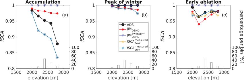
N. Helbig et al.: A seasonal algorithm of the snow-covered area fraction for mountainous terrain                                4611

                                                                        four additional snow cover simulations: JIMseason     curr
                                                                                                                    OSHD , JIMOSHD ,
                                                                            allHelbig
                                                                        JIMOSHD and JIMSwenson*
                                                                                            OSHD     (see Table 1).

                                                                        3.2     Evaluation data

                                                                        3.2.1    ADS fine-scale HS maps

                                                                        We used fine-scale spatial HS maps gathered by airborne dig-
                                                                        ital scanning (ADS) with an optoelectronic line scanner on an
                                                                        airplane. Data were acquired over the Wannengrat and Dis-
                                                                        chma area near Davos in the eastern Swiss Alps during win-
                                                                        ter and summer (Bühler et al., 2015). We used ADS-derived
Figure 2. Illustration of modeled fSCArecent             14 d
                                            nsnow , fSCAnsnow and
fSCAseason for one grid cell over a season. The fSCA is the
                                                                        HS maps at three points in time during one winter season,
maximum for each time step from fSCAnsnow = max(fSCArecent              namely during accumulation on 26 January (acc), at approx-
                                                              nsnow ,
fSCA14  d                                                               imate peak of winter on 9 March (PoW) and during ablation
     nsnow ) and fSCAseason . All terms are described in Sect. 2.2.
                                                                        season on 20 April 2016 (abl) (Marty et al., 2019). We used
                                                                        a summer DEM from ADS to derive the snow-free terrain
latter model combination is used to predict daily snow mass             parameters.
and snowpack runoff for the operational snow hydrology ser-                Each ADS data set covers about 150 km2 at 2 m spatial res-
vice (OSHD) at WSL Institute of Snow and Avalanche Re-                  olution. Compared to TLS-derived (terrestrial laser scan) HS
search SLF. We ran JIMOSHD at 1 km resolution with hourly               data, the 2 m ADS-derived HS maps had a root mean square
meteorological data from the COSMO-1 model (operated by                 error (RMSE) of 33 cm and a normalized median absolute
MeteoSwiss) for Switzerland. We used a reanalysis product               deviation (NMAD) of 24 cm (Bühler et al., 2015).
of daily observed precipitation (RhiresD) from MeteoSwiss,
                                                                        3.2.2    ALS fine-scale HS maps
as well as COSMO-1 data. Daily HS measurements from
manual observers, as well as from a dense network of auto-              We used fine-scale spatial HS maps gathered by airborne
matic weather stations (AWSs), were used to correct precip-             laser scanning (ALS). The ALS campaign was a Swiss
itation data via optimal interpolation (OI) (Magnusson et al.,          partner mission of the Airborne Snow Observatory (ASO)
2014), which is a computationally efficient data assimilation           (Painter et al., 2016). Lidar setup and processing standards
approach. Using OI in JIMOSHD , Griessinger et al. (2019)               were similar to those in the ASO campaigns in California.
obtained improved discharge simulations in 25 catchments                Data were acquired over the Dischma area near Davos in the
over 4 hydrological years.                                              eastern Swiss Alps (see Fig. 3a in Helbig et al., 2021a). We
   To describe the subgrid snow cover evolution in mountain-            used ALS-derived HS maps at three points in time during one
ous terrain, our seasonal fSCA algorithm was implemented                winter season, namely at the approximate peak of winter on
in JIMOSHD . As daily values, we used model output gener-               20 March (PoW) and during the early and late ablation sea-
ated at 06:00 (UTC). In the following, modeled fSCA and                 son on 31 March and 17 May 2017 (abl), respectively. We
HS maps refer to daily fSCA and HS from JIMOSHD model                   used a summer DEM from ALS from 29 August 2017 to de-
output.                                                                 rive the snow-free terrain parameters.
   We also computed the snow cover evolution using                         Each ALS data set covered about 260 km2 . The original
JIMOSHD with various simplifications in the seasonal fSCA               3 m resolution was aggregated to 5 m horizontal resolution.
algorithm, as well as with the fSCA parameterizations imple-            Comparing the ALS-derived HS data to manual snow prob-
mented in CLM5.0 (Lawrence et al., 2018), which are based               ing within forest but outside canopy (i.e., not below a tree),
on Swenson and Lawrence (2012) (see Table 1 for more                    Mazzotti et al. (2019) reported a RMSE of 13 cm and a bias
details). This latter fSCA algorithm also accounts for hys-             of −5 cm for 20 March 2017.
teresis in accumulation and ablation by using two different
fSCA parameterizations and by tracking the seasonal max-                3.2.3    Terrestrial camera images
imum SWE. While subgrid topography is accounted for in
the fSCA parameterization during ablation via σz , topogra-             We used camera images from terrestrial time-lapse photog-
phy is not accounted for during snowfall events. The algo-              raphy in the visible band. The camera (Nikon Coolpix 5900
rithm of Swenson and Lawrence (2012) was derived by link-               from 2016 to 2018, Canon EOS 400D from 2019 to 2020)
ing daily satellite-retrieved fSCA to snow data. We imple-              was installed at the SLF/WSL in Davos Dorf in the eastern
mented this algorithm in JIM using our snow tracking algo-              Swiss Alps (van Herwijnen and Schweizer, 2011; van Her-
rithm, i.e., the corresponding HS values such as HSpseudo-min           wijnen et al., 2013). Photographs were taken of the Dorfberg
(see Sect. 2.2). This was done to solely evaluate the differ-           in Davos, which is a large southeast-facing slope with a mean
ences in the fSCA parameterizations. In total, we performed             slope angle of about 30◦ (see Fig. 1 in Helbig et al., 2015a).

https://doi.org/10.5194/tc-15-4607-2021                                                      The Cryosphere, 15, 4607–4624, 2021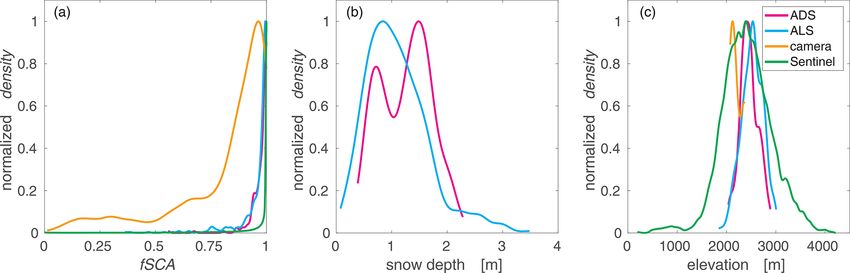
4612                     N. Helbig et al.: A seasonal algorithm of the snow-covered area fraction for mountainous terrain

Table 1. Details of the different fSCA algorithms that are compared to the full fSCA algorithm in JIMOSHD .

        Algorithm name      fSCAseason                   fSCAnsnow                         Tracking HS and SWE (Sect. 2.2)
        JIMOSHD             Eq. (5)                      Eqs. (6) and (7)                  Season and 14 d
        JIMseason
           OSHD             Eq. (5)                  !   –                                 Season

        JIMcurr
           OSHD             tanh   1.3 HS current
                                        Helbig           –                                 –
                                       σHS
                                           current
            allHelbig                                                             Helbig
        JIMOSHD             Eq. (5)                      Eqs. (6) and (7) with σHS         Season and 14 d
        JIMSwenson*
           OSHD             Eq. (8.2) in                 Eq. (8.1) in                      Season and 14 d
                            Lawrence et al. (2018)       Lawrence et al. (2018)

To obtain fSCA values from the camera images, we followed                   3.3    Derivation of 1 km fSCA evaluation data
the workflow described by Portenier et al. (2020). We used
the algorithm of Salvatori et al. (2011) to classify pixels in              For pre-processing, we masked out forest, rivers, glaciers
the images as snow or snow-free. Though images are taken                    or buildings in all fine-scale measurement data sets. Optical
at regular intervals (between 2 and 15 min, depending on the                snow products that were obscured by clouds were also omit-
year), we used the image at noon to derive fSCA for that                    ted. In all fine-scale HS data sets, we neglected HS values
day. We evaluated images from five winter seasons (2016,                    that were lower than 0 or above 15 m. We used a HS threshold
2017, 2018, 2019 and 2020) every time from 1 November to                    of 0 m to decide whether or not a 2 or 5 m grid cell was snow-
30 June.                                                                    covered. This threshold could not be better adjusted due to a
   The resulting snow/no-snow map of the camera images                      lack of independent observations.
had a horizontal resolution of 2 m. The field of view (FOV)                    We then aggregated all fine-scale snow data, as well as the
overlaps with four 1 × 1 km JIMOSHD grid cells with pro-                    snow products from optical imagery, in squared domain sizes
jected visible fractions between 9 % to 40 % in each grid cell.             L in regular grids of 1 km aligned with the OSHD model do-
The camera FOV covers about 0.76 km2 .                                      main. For the spatial averages, we required at least 70 % valid
                                                                            data for the fine-scale snow data and at least 50 % valid for
3.2.4   Sentinel-2 snow products                                            the satellite-derived fSCA data in each 1 km grid cell. We ex-
                                                                            cluded 1 km grid cells with spatial mean slope angles larger
We used fine-scale snow-covered area maps obtained from
                                                                            than 60◦ and spatial mean measured or modeled HS < 5 cm.
the Theia snow collection (Gascoin et al., 2019). The satel-
                                                                            We further neglected 1 km grid cells with forest fractions
lite snow products were generated from Sentinel-2 L2A and
                                                                            larger than 10 %, derived from 25 m forest cover data. Over-
L2B images. We used Sentinel-2 snow-covered area maps
                                                                            all, this led to a variable number of 1 km valid grid cells for
over one winter season from 20 December 2017 to 31 Au-
                                                                            the different data sets (Table 2). For the fine-scale snow data
gust 2018 for Switzerland. We further used Sentinel-2 snow
                                                                            sets, this number ranged from 69 to 157 with a total of 668
maps over the Dischma area near Davos close to or on
                                                                            valid 1 km grid cells. After cloud and forest removal, on av-
the date of the three ALS scans (18 and 28 March and
                                                                            erage, every second day we had some valid Sentinel-2 data in
17 May 2017) and over the Dorfberg area in Davos Dorf from
                                                                            Switzerland (153 valid days from the 255 calendar days). For
1 November 2017 to 30 June 2018.
                                                                            the time period from 20 December 2017 to 31 August 2018,
   The horizontal resolution of the snow product is 20 m.
                                                                            this resulted in 216 896 valid 1 km grid cells from a total of
While the spatial coverage of the Sentinel-2 snow-covered
                                                                            2 274 991 valid OSHD grid cells in Switzerland, i.e., about
area maps in Switzerland varies every time step, Sentinel-
                                                                            9.5 %.
2 may cover several thousand square kilometers. A valida-
                                                                               These valid 1 km grid cells covered terrain elevations from
tion of the Theia snow product with snow depth from AWSs,
                                                                            174 to 4278 m, subgrid mean slope angles from 0 to 60◦
through a comparison to snow maps with higher spatial res-
                                                                            and all terrain aspects. We used three of the four grid cells
olution, as well as by visual inspection, indicated that snow
                                                                            covered by the FOV of the terrestrial camera since one grid
is well detected, although there is a tendency to underdetect
                                                                            cell had a forest fraction larger than 10 %. On average, every
snow (Gascoin et al., 2019). The main difficulty of satel-
                                                                            fourth day we had valid camera data (337 valid days from
lite snow products is to avoid false snow detection within
                                                                            the 1212 calendar days). Valid camera-derived fSCA for five
clouds. Furthermore, snow omission errors may occur on
                                                                            seasons and the three grid cells covered by the FOV resulted
steep, shaded slopes when the solar elevation is typically be-
                                                                            in 931 valid 1 km grid cells from a total of 3018 valid OSHD
low 20◦ .
                                                                            grid cells, i.e., 31 %. The three grid cells have terrain eleva-
                                                                            tions of 2077, 2168 and 2367 m and slope angles of 27, 34
                                                                            and 39◦ . The diversity in each of the evaluation data sets af-

The Cryosphere, 15, 4607–4624, 2021                                                              https://doi.org/10.5194/tc-15-4607-2021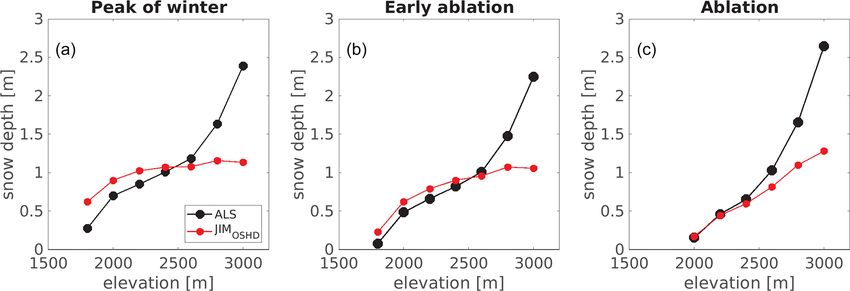
N. Helbig et al.: A seasonal algorithm of the snow-covered area fraction for mountainous terrain 4613
Figure 3. Probability density functions after preprocessing for all valid 1 km (a) fSCA, (b) snow depth and (c) elevation per measurement
data set. All densities were normalized with the maximum in each data set. Colors represent the different measurement platforms as detailed
in Sect. 3.2.
Table 2. Details of the valid 1 km fSCA evaluation data sets after pre-processing as described in Sect. 3.3.
Geographical region Remote Spatial Temporal σfSCA Mean fSCA
sensing method coverage coverage
[km2 ] [days]
Wannengrat and Dischma area (eastern CH) ADS 232 3 0.05 0.98
Dischma and Engadin area (eastern CH) ALS 436 3 0.08 0.96
Davos Dorfberg (eastern CH) Terrestrial camera 931 337 0.23 0.81
Switzerland Sentinel-2 216 896 153 0.18 0.93
ter pre-processing is indicated in Table 2 and is also shown 4.1 Evaluation with fSCA from fine-scale HS maps
for valid 1 km domains by means of the probability density
function (pdf) for fSCA, HS and terrain elevation z in Fig. 3. Modeled fSCA compared well with fSCA derived from all
six fine-scale HS data sets. Overall, we obtained a NRMSE
3.4 Performance measures
of 7 %, a RMSE of 0.07 and a MPE of 0.7 % (Table 3). The
To evaluate the performance of modeled fSCA compared to best performance was for the two dates at the approximate
the measurements, we used three measures: the root mean PoW (NRMSE of 2 %, a RMSE of 0.02 and a MPE of 0.3 %),
square error (RMSE), the normalized root mean square error while the performance was somewhat lower during the abla-
(NRMSE; normalized by the mean of the measurements) and tion and accumulation periods.
the mean percentage error (MPE; defined as measured minus To investigate the influence of elevation, we binned the
modeled, normalized with the mean of the measurements). data in 200 m elevation bands for the ADS and ALS data
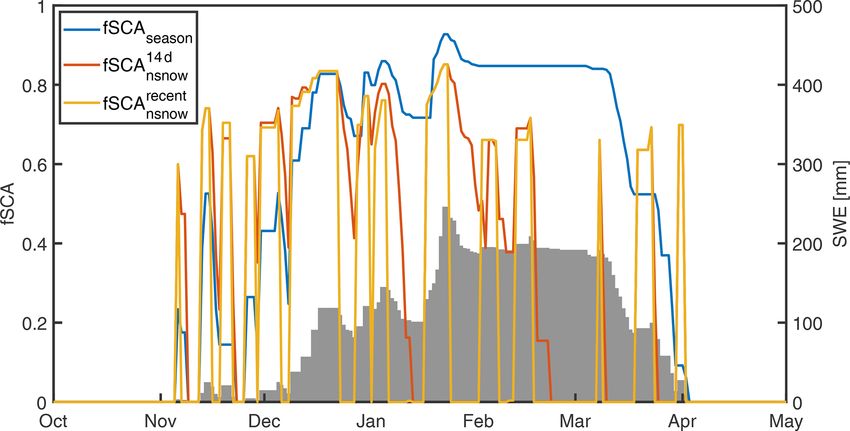
sets separately (Figs. 4 and 5). For ADS data, elevation-
dependent modeled fSCA values were comparable to the
4 Results measurements at PoW and early ablation, while the differ-
ences during accumulation were more pronounced (compare
We present the evaluation of our seasonal fSCA algorithm red and black dots in Fig. 4). There was also no consistent
in three sections: evaluation with fSCA derived from fine- elevation trend, as during accumulation differences between
scale HS maps near Davos, evaluation with fSCA from time- modeled and measured fSCA increased with elevation, while
lapse photography in Davos Dorf and evaluation with fSCA during early ablation the opposite was true. For the ALS
from Sentinel-2 snow products over Switzerland. We further data, measurements were only available at PoW and dur-
present some additional comparisons with Sentinel-2 snow ing ablation. Overall, modeled fSCA values were again in
products in the first two sections when Sentinel-2 data were line with the measurements (compare red and black dots in
available in the Davos area (see Sect. 3.2.4). Fig. 5). The largest difference was observed for the lowest-
elevation bin (0.15 at PoW at 1800 m; Fig. 5a), and for the
late ablation data, modeled fSCA was consistently lower than
ALS-derived fSCA, in particular for the lower-elevation bins
(Fig. 5c).
https://doi.org/10.5194/tc-15-4607-2021 The Cryosphere, 15, 4607–4624, 2021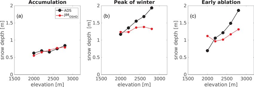
4614                       N. Helbig et al.: A seasonal algorithm of the snow-covered area fraction for mountainous terrain

Table 3. Performance measures for modeled fSCA with (I) fSCA           fSCAmeasured
                                                                             PoW      (orange stars in Figs. 4 and 5) combines cur-
derived from all fine-scale HS maps (combined ADS- and ALS-            rent HS measurements with σHS values measured at PoW.
derived fSCA) and (II) Sentinel-derived fSCA (only available for       At PoW, fSCAmeasured
                                                                                        PoW     and fSCAmeasured
                                                                                                            curr    are the same, and
ALS dates). Additionally, performance measures are shown for                 measured
                                                                       fSCAPoW        can only be derived at or after PoW. Results
ALS-derived fSCA with Sentinel-derived fSCA (III) and for mod-         obtained with both benchmark models were similar except
eled fSCA using JIMSwenson*     (IV). Given statistics are NRMSE,
                        OSHD                                           for the lowest-elevation bin in the ALS data set (Fig. 5b and
RMSE and MPE. For all differences we computed measured minus
modeled values respectively Sentinel-derived fSCA minus ALS-
                                                                       c). Overall, the values of fSCAmeasured
                                                                                                       curr      were somewhat closer
derived fSCA for III. The different points in time of the season are   to the measured fSCA values (e.g., Figs. 4c or 5b). Both
specified in Sect. 3.2.                                                benchmark models were closest to the measured fSCA val-
                                                                       ues during the ablation season (Figs. 4c and 5c), and overall
 fSCA                                       NRMSE   RMSE     MPE       the agreement was better for higher-elevation bins. Our sea-
                                              [%]             [%]
                                                                       sonal fSCA implementation (red dots in Figs. 4 and 5) was
                                                                       also similar to both benchmark models. The largest differ-
 I JIMOSHD vs. ADS&ALS
                                                                       ences were during the accumulation period (Fig. 4a).
 All dates                                      7     0.07    0.7         As a final benchmark, we also compared our seasonal
 Accumulation date                              8     0.08   −3.8      fSCA implementation with the parameterizations imple-
 PoW dates                                      2     0.02    0.3
 Ablation dates                                 8     0.08    1.8      mented in CLM5.0 (see Table 1). Modeled fSCA us-
                                                                       ing JIMOSHD performed better than that modeled with
 II JIMOSHD vs. Sentinel-2 (at ALS dates)
                                                                       JIMSwenson*
                                                                            OSHD     (compare I and IV in Table 3). During most of
 All dates                                      9     0.08   −1.4      the season, fSCA values from JIMSwenson*
                                                                                                              OSHD     were close to 1
 PoW dates                                      3     0.03    2.5
                                                                       and showed little elevation dependence (blue stars in Figs. 4
 Ablation dates                                 9     0.08   −1.5
                                                                       and 5). The only exception was during the late-ablation sea-
 III Sentinel-2 vs. ALS                                                son, when fSCA values from JIMOSHD and from JIMSwenson*OSHD
 All dates                                     11     0.10    3.1      were very similar (red dots and dark blue stars in Fig. 5c).
 PoW date                                       9     0.08   −5.9         To investigate the origin of the discrepancies between
 Ablation dates                                11     0.10    3.4
                                                                       modeled and observed fSCA values more closely, we com-
 IV JIMSwenson*
       OSHD     vs. ADS&ALS                                            pared modeled and measured HS in 200 m elevation bins
 All dates                                     14     0.14   −1.2      for the ADS and ALS data sets separately (Figs. 6 and 7).
 Accumulation date                              9     0.09   −6.1      For both data sets, modeled HS was substantially lower than
 PoW dates                                      6     0.06   −0.6      measured HS at higher elevations. The only exception was
 Ablation dates                                18     0.18   −0.7
                                                                       for the accumulation date, when modeled and measured HS
                                                                       values were in good agreement for all elevations (Fig. 6a).
                                                                       For all dates and data sets, the NRMSE between modeled
   Valid Sentinel-2 data were only available on dates close            and measured HS was 12 %, and the MPE was 14 %. Note
to the ALS measurements (green dots in Fig. 5), not to the             that seasonal variations in ALS HS across all elevations were
ADS measurement dates. Overall, modeled and Sentinel-                  generally much lower than those in the ADS HS data. This
derived fSCA values were in good agreement for the three               was in part because the time intervals between the three
ALS dates (II in Table 3), there was no clear elevation de-            ALS scans (20 March, 31 March and 17 May 2017) were
pendence (compare green and red dots in Fig. 5), and dif-              shorter than for the ADS scans (26 January, 9 March and
ferences were at most 0.05 (for elevations between 2300 and            20 April 2016), and there were also some snowfall events
2500 m in Fig. 5c). The Sentinel-derived fSCA values can               during the ALS ablation period (spring 2017).
also be compared to those from the ALS scans. In this case,
the performance measures were somewhat lower (compare II               4.2   Evaluation with fSCA from camera images
and III in Table 3), and Sentinel-derived fSCA values were
especially lower than the ALS data in late ablation (compare           The high temporal resolution of camera-derived fSCA al-
green and black dots in Fig. 5c).                                      lowed us to evaluate the seasonal model performance. The
   Our seasonal fSCA algorithm is implemented in a com-                seasonal trend in modeled fSCA using JIMOSHD was gen-
plex operational snow cover model framework (Sect. 3.1).               erally in line with that from camera-derived fSCA (compare
Uncertainties related to input or model structure therefore            red and black dots in Fig. 8). For the grid cell at 2168 m, how-
impact modeled HS and fSCA values. To investigate the                  ever, the agreement was somewhat poorer as there was a de-
influence of these uncertainties more closely, we also de-             lay in the modeled start of the ablation season, and modeled
rived two benchmark fSCA models based on Eq. (1) using                 fSCA values were too high during accumulation (Fig. 8b, e).
measured rather than modeled HS data. The first benchmark                 For all winter seasons (2016 to 2020) and for the three grid
fSCAmeasured
      curr    (light blue stars in Figs. 4 and 5) uses measured        cells, we obtained a NRMSE of 21 %, a RMSE of 0.17 and a
HS and σHS from the current scan. The second benchmark                 MPE of −7 % (I in Table 4). Note that the inter-annual per-

The Cryosphere, 15, 4607–4624, 2021                                                       https://doi.org/10.5194/tc-15-4607-2021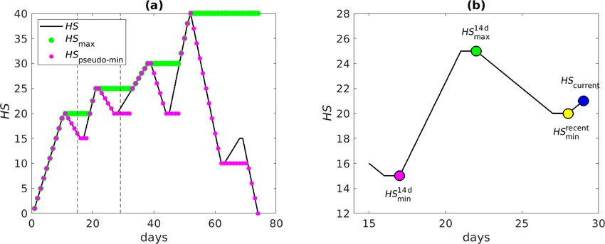
N. Helbig et al.: A seasonal algorithm of the snow-covered area fraction for mountainous terrain                                        4615

Figure 4. Modeled and ADS-derived fSCA in 200 m elevation bins for three dates: (a) during accumulation, (b) at approximate peak of
winter (PoW) and (c) during ablation. Two benchmarks based on Eq. (1) are shown where applicable: fSCAmeasured
                                                                                                         PoW     (orange stars) uses HS
form from the current ADS scan and σHS from the ADS scan at PoW, while fSCAmeasured
                                                                             curr   (light blue stars) uses HS and σHS from the current
ADS scan. The bars show the valid data percentage per bin.

Figure 5. Modeled and ALS-derived, as well as Sentinel-derived, fSCA in 200 m elevation bins for three dates: (a) at approximate PoW,
(b) during early ablation and (c) during late ablation. The same two benchmarks based on Eq. (1) as in Fig. 4 are also shown where applicable.
Sentinel-derived fSCA (green dots) was available 2 d before the PoW scan, 3 d before the early ablation scan and on the same day as the late
ablation scan. The bars show the valid data percentage per bin.

formance varied substantially, as did the performance among              agreed well, there were substantial differences after snow-
the three grid cells. For instance, for all three grid cells, the        fall events on partly snow-free ground (compare orange stars
overall best performance was for the season 2018 (NRMSE                  and red dots in Fig. 8). Specifically, after such a snowfall
= 14 %, RMSE = 0.11, MPE = −4 %), while the worst per-                   event, modeled fSCA using JIMOSHD generally increased,
formance was for the season 2019 (NRMSE = 25 %, RMSE                     while JIMseason                                      curr
                                                                                     OSHD remained constant. Using JIMOSHD , mod-
= 0.2, MPE = −12 %).                                                     eled fSCA values were less in line with those from JIMOSHD
   For winter season 2018, we used Sentinel-derived fSCA                 (compare light blue stars and red dots in Fig. 8). While dis-
to evaluate modeled and camera-derived fSCA values. While                crepancies were again large after snowfall events, they were
overall the agreement between modeled and Sentinel-derived               also pronounced during the ablation periods. In general, with
fSCA was good (NRMSE 2 % and MPE of 1 %), the                            JIMcurr
                                                                              OSHD the ablation season started later and was followed
agreement between camera- and Sentinel-derived fSCA was                  by a much steeper melt-out period. Using JIMcurr  OSHD can result
poorer (NRMSE = 12 %, MPE = 5 %). The latter per-                        in a substantially shorter snow season compared to JIMOSHD ,
formance values were, however, comparable to the agree-                  with a maximum difference of 21 d at 2168 m in the season
ment between modeled and camera-derived fSCA for days                    2017. Overall, compared to camera-derived fSCA, both sim-
with valid Sentinel-derived data (NRMSE = 12 %, MPE =                    plified models performed less well than JIMOSHD (Table 4).
−4 %).                                                                                                 allHelbig
                                                                         The performance using JIMOSHD was very similar to fSCA
   The camera-derived fSCA was also used to evaluate the                 from JIMOSHD ; i.e., applying σHS
                                                                                                               Helbig              Egli
                                                                                                                      instead of σHS for
relevance of applying our full seasonal fSCA algorithm as                fSCAnsnow did not substantially affect model performance.
opposed to simplifications and JIMSwenson*
                                      OSHD      (see Table 1 for         On the contrary, fSCA from JIMSwenson*        had the worst over-
                                                                                                             OSHD
details). While overall fSCA from JIMseasonOSHD and JIMOSHD              all performances when compared to camera-derived fSCA

https://doi.org/10.5194/tc-15-4607-2021                                                          The Cryosphere, 15, 4607–4624, 2021
4616 N. Helbig et al.: A seasonal algorithm of the snow-covered area fraction for mountainous terrain
Figure 6. Modeled and ADS-derived HS in 200 m elevation bins for three dates: (a) during accumulation, (b) at approximate PoW and
(c) during ablation.
Figure 7. Modeled and ALS-derived HS in 200 m elevation bins for three dates: (a) at approximate PoW, (b) during early ablation and
(c) during ablation.
(VII in Table 4). Similar to JIMcurr Swenson* con-
OSHD , using JIMOSHD evation throughout the season. Up to the end of the accumu-
siderably delayed the ablation season, followed by a much lation period, the largest differences between modeled and
steeper melt out. The snow season was substantially short- Sentinel-derived fSCA were at elevations lower than 1500 m,
ened again by at most 32 d in the 2017 season at 2077 m. whereas at elevations above around 3000 m, the agreement
Modeled fSCA using JIMSwenson*
OSHD also largely overestimates was good (Fig. 9a). During the ablation period, most of the
fSCA during the accumulation period (blue dots in Fig. 8). snow at lower elevations was gone, and modeled fSCA was
Overall, using JIMSwenson*
OSHD led to much steeper increases generally larger than Sentinel-derived fSCA at higher eleva-
and decreases in fSCA, i.e., an almost binary seasonal fSCA tions (> 2500 m), in particular towards the end of the abla-
trend that was not in line with camera-derived fSCA. tion season. During the summer (30 June to 30 August 2018),
i.e., after the end of the ablation season, modeled fSCA was
4.3 Evaluation with fSCA from Sentinel-2 snow larger than Sentinel-derived fSCA at the highest elevations
products (> 3500 m), whereas between the snow line and these high-
est elevations, modeled fSCA was generally lower.
Overall, modeled fSCA using JIMOSHD compared well with Given the high temporal resolution of the Sentinel-derived
Sentinel-derived fSCA throughout the season (I in Table 5). fSCA data set, we again evaluated the fSCA algorithm sim-
To investigate the elevation-dependent differences between plifications and JIMSwenson*
OSHD (see Table 1). Compared to our
modeled and Sentinel-derived fSCA in more detail, we seasonal implementation, the overall performance values of
binned the data in 250 m elevation bands for each day the fSCA algorithm simplifications were similar except for
throughout the entire season (Fig. 9). To estimate the end JIMcurr
OSHD and JIMOSHD
Swenson* (Table 5). Modeled fSCA val-
of the accumulation (1 April 2018) and ablation season ues with JIMOSHD and JIMSwenson*
curr
OSHD were generally larger
(30 June 2018), we used the spatial mean HS (solid black line than Sentinel-derived fSCA, resulting in larger MPE values
at bottom of Fig. 9). Overall, differences in performance be- with the largest ones for JIMSwenson*
OSHD (compare I, III and V
tween the accumulation and the ablation period were small (I in Table 5). This is also clearly reflected in the elevation-
in Table 5). However, there were marked differences with el-
The Cryosphere, 15, 4607–4624, 2021 https://doi.org/10.5194/tc-15-4607-2021N. Helbig et al.: A seasonal algorithm of the snow-covered area fraction for mountainous terrain 4617
Figure 8. Modeled and camera- and Sentinel-derived fSCA for the three 1 km grid cells within the field of view of the camera for two
seasons: (a–c) winter 2017 and (d–f) winter 2018.
Egli
dependent differences between fSCA using JIMSwenson*
OSHD and We used σHS (Eq. 4), which does not account for subgrid
Sentinel-derived fSCA throughout the season (Fig. 9b). topography, to derive fSCAnsnow . We did this to account for
uniform blanketing after a snowfall, i.e., to account for pos-
sible increases in fSCA after a recent snowfall. When sub-
5 Discussion Egli Helbig allHelbig
stituting σdHS with σdHS in Eqs. (6) and (7) (JIMOSHD ;
see Table 1), the overall performance was very similar (Ta-
5.1 Fractional snow-covered area fSCA algorithm Egli
bles 4 and 5). Thus, while applying σdHS might not describe
Our seasonal fSCA algorithm is based on the closed-form the true spatial new snow distribution in mountainous ter-
fSCA parameterization of Helbig et al. (2015a) (Eq. 1) and rain, the formulation is simple and is therefore used here as
combines two statistical parameterizations for σHS , together a first approach. Based on the modular algorithm setup, dif-
with a tracking method, to account for changes in maxi- ferent closed-form fSCA parameterizations can be applied
mum snow depth and precipitation events. The algorithm is in our seasonal algorithm, e.g., for a flat grid cell or for
modular, meaning that individual parts can easily be com- fSCAnsnow (for some empirical examples, see Essery and
plemented or replaced with new parameterizations, e.g., for Pomeroy, 2004).
fSCAnsnow . Overall, our algorithm only requires subgrid cell
summer terrain parameters, which are a slope-related param- 5.2 Evaluation
eter and the terrain correlation length, and tracking snow in-
5.2.1 Evaluation with fSCA from fine-scale HS maps
formation.
We evaluated the performance of our seasonal fSCA im- The evaluation of the seasonal fSCA algorithm with fSCA
plementation in Switzerland. We could not explicitly eval- from fine-scale HS maps showed that overall the model per-
uate the performance for completely flat grid cells, i.e., grid formed well, especially at PoW (I in Table 3). Modeled
cells with a subgrid mean slope angle of zero. After removing fSCA using JIMSwenson*
OSHD , on the other hand, generally over-
rivers/lakes, we only had five 1 km grid cells for Switzerland estimated fSCA (MPE< 0). This algorithm intercomparison
with a subgrid mean slope angle of zero, i.e., 0.01 % of all shows that the seasonal fSCA evolution is better captured by
Helbig
grid cells. For these grid cells, using σHS (Eq. 2) always JIMOSHD most likely because the JIMSwenson*
OSHD model does
results in a fSCA of 1. As a first approach, we therefore pro- not sufficiently account for the high spatial variability in
Egli
posed to use σHS (Eq. 4). Although we see no reason why snow distribution in complex terrain.
our fSCA algorithm could not be used in other geographic During accumulation at higher elevations, modeled fSCA
region, it remains unclear at this point if our seasonal fSCA using JIMOSHD overestimated ADS-derived fSCA even
implementation can also be used in flat regions. though modeled HS agreed reasonably well with the mea-
https://doi.org/10.5194/tc-15-4607-2021 The Cryosphere, 15, 4607–4624, 20214618 N. Helbig et al.: A seasonal algorithm of the snow-covered area fraction for mountainous terrain
Figure 9. Difference between Sentinel-derived and modeled fSCA for Switzerland as a function of date and elevation z (in 250 m elevation
bins) for available satellite dates for (a) JIMOSHD and (b) JIMSwenson*
OSHD . Daily spatial mean snow depth HS is also shown (solid black line).
The vertical lines indicate the dates for the end of accumulation (dashed) and ablation (line with stars) seasons.
surements (Figs. 4a and 6a). We also used a different model
allHelbig
configuration (JIMOSHD in Table 1), yet fSCA values
Table 4. Performance measures for (I) modeled fSCA using did not substantially change for the accumulation date (not
JIMOSHD and camera-retrieved fSCA for the winter seasons 2016 shown). Based on this we assume that both σHS parameteri-
to 2020, (II) modeled fSCA using JIMOSHD and Sentinel-derived zations cannot sufficiently describe snow redistribution dur-
fSCA for the three grid cells for the winter season 2018, (III) ing accumulation likely due to periods with strong winds fol-
camera-derived fSCA with Sentinel-derived fSCA for the three grid lowing snowfall. The description of σHS during the accumu-
cells, and (IV to VII) all JIM-modeled fSCA versions (for details
allHelbig lation period thus needs to be improved. This will, however,
see Table 1), namely for JIMseason curr
OSHD , JIMOSHD , JIMOSHD and
require more than one spatial HS data set during accumula-
JIMSwenson*
OSHD , with camera-derived fSCA. tion.
At PoW and during the ablation season, JIMOSHD mostly
fSCA NRMSE RMSE MPE underestimated fSCA compared to fSCA from fine-scale HS
[%] [%] maps, without a clear elevation trend (Figs. 4 and 5). Dis-
crepancies between modeled and measured HS, on the other
I JIMOSHD vs. camera hand, generally increased with elevation (Figs. 6 and 7). Ob-
21 0.17 −7.1 viously for larger snow depth, correctly modeling HS has
little effect on fSCA. The overall underestimated modeled
II JIMOSHD vs. Sentinel-2
fSCA values were likely a consequence of the HS threshold
2 0.02 0.8 of 0 m we used to decide whether a 2 or 5 m grid cell was
III Camera vs. Sentinel-2 snow-covered or not. In reality, due to measurement uncer-
tainties, both small positive or negative measured HS values
12 0.11 5.0 can still be associated with snow-free areas. When arbitrar-
IV JIMseason ily increasing the HS threshold to ±10 cm for the ALS data,
OSHD vs. camera
modeled 1 km fSCA values were rather larger than the mea-
22 0.18 −6.1 surements (not shown). This is not contradictory but empha-
V JIMcurr
OSHD vs. camera
sizes the need to accurately model HS along snow lines, in
which small inaccuracies in HS can have large impacts on
26 0.21 −9.2
fSCA. For instance, during early ablation modeled and mea-
allHelbig sured fSCAs are larger in the lowest-elevation bin than at
VI JIMOSHD vs. camera
higher elevations (see Fig. 4c). Unfortunately, we currently
21 0.17 −7.6
do not have detailed snow observations available to define
VII JIMSwenson*
OSHD vs. camera robust HS threshold values which take into account the dif-
ferent points in time of the season, as well as the influence of
30 0.25 −10.6
terrain and ground cover. However, the overall good agree-
ment between Sentinel- and ALS-derived fSCA (Fig. 5 and
The Cryosphere, 15, 4607–4624, 2021 https://doi.org/10.5194/tc-15-4607-2021N. Helbig et al.: A seasonal algorithm of the snow-covered area fraction for mountainous terrain 4619
Table 5. Performance measures (I) for modeled fSCA using sured σHS at the date we defined as PoW might not have been
JIMOSHD and Sentinel-retrieved fSCA for the winter season 2018 representative for the true σHSmax in each grid cell as required
for all valid 1 km grid cells of Switzerland and for all dates (20 De- by Eq. (5). Besides possible uncertainties in the empirical
cember 2017 to 30 June 2018), for the accumulation period (20 De- fSCA parameterization (Eq. 1), we assume this is the main
cember to 1 April), and for the ablation period (1 April to 30 June), reason why these two benchmark models using measured HS
as well as (II to V) for all JIM-modeled fSCA versions (for de-
data did not outperform our seasonal implementation. Over-
tails, see Table 1), namely for JIMOSHD , JIMseason curr
OSHD , JIMOSHD ,
allHelbig all, these comparisons emphasize the need for tracking snow
JIMOSHD and JIMSwenson*
OSHD . information per grid cell, as is done by our seasonal fSCA
algorithm.
fSCA vs. Sentinel-2 NRMSE RMSE MPE
[%] [%] 5.2.2 Evaluation with camera-derived fSCA
I JIMOSHD The evaluation with fine-scale HS maps revealed overall
All dates 12 0.11 0.4 good model performance at six points in time. It was, how-
Accumulation period 11 0.11 0.3 ever, not possible to comprehensively evaluate the perfor-
Ablation period 14 0.12 0.5 mance over the season. For this, we used daily camera-
II JIMseason derived fSCA, showing that the modeled seasonal fSCA
OSHD
trend was mostly in line with observations (Fig. 8).
All dates 12 0.12 0.4 Model performance compared to the camera-derived
Accumulation period 11 0.11 0.3 fSCA values was overall worse than when comparing to HS-
Ablation period 14 0.12 0.5 derived fSCA (e.g., NRMSE of 21 % for I in Table 4 com-
III JIMcurr
OSHD
pared to NRMSE of 7 % for I in Table 3). Since the higher
temporal resolution of the camera data set leads to the largest
All dates 14 0.13 −0.8
spread in fSCA values compared to the other two data sets
Accumulation period 11 0.11 0.1
Ablation period 18 0.16 −2.4 (see Table 2 and Fig. 3), a larger portion of intermediate
fSCA values (e.g., close to the snow line) are included which
allHelbig
IV JIMOSHD are generally more difficult to model correctly than fSCA
values close to 1. The poorer model performance is, how-
All dates 12 0.11 0.3
Accumulation period 11 0.11 0.2 ever, likely also due to the overall lower accuracy of camera-
Ablation period 14 0.12 0.5 derived fSCA. For instance, the projection of the 2D cam-
era image to a 3D DEM may introduce errors and distor-
V JIMSwenson*
OSHD tions. Furthermore, when deriving fSCA from camera im-
All dates 18 0.17 −1.8 ages, clouds/fog and uneven illumination, for instance due
Accumulation period 17 0.16 −0.7 to shading or partial cloud cover, may deteriorate the accu-
Ablation period 21 0.19 −3.6 racy (e.g., Farinotti et al., 2010; Fedorov et al., 2016; Härer
et al., 2016; Portenier et al., 2020). Another factor affecting
the performance measures was the threshold for the number
of valid fine-scale data per 1 km grid cell. When aggregating
III in Table 3) provides some confidence in the fine-scale HS to 1 km fSCA maps for the Sentinel-derived values, we re-
data-derived fSCA used here to evaluate modeled fSCA. quired at least 50 % valid fine-scale data. This requirement
The two benchmark fSCA models based on Eq. (1) us- could not be met for camera-derived fSCA as the projected
ing measured rather than modeled HS data (fSCAmeasured
curr and fractions of the camera FOV on the 1 km model grid cells
fSCAmeasured
PoW ) generally showed similar trends as HS-derived were only 9 %, 13 % and 14 %. This is reflected in the bet-
and modeled fSCA (Figs. 4 and 5). At PoW, fSCAmeasured curr ter agreement between modeled and Sentinel-derived fSCA
agreed less well with measured fSCA than our seasonal im- than between camera- and Sentinel-derived fSCA (NRMSE
plementation (see Figs. 4b and 5a). This may indicate un- of 2 % vs. 12 % in Table 4). Finally, as the camera was in-
certainties in the empirical fSCA parameterization (Eq. 1), stalled at valley bottom, steep slope sections cover larger
which requires the further investigation of spatial HS data areas of the FOV, while flatter slope parts remain invisible.
sets during accumulation. During ablation, we expected This likely led to underestimated fSCA values. On the other
that fSCAmeasured
PoW would be closer to measured fSCA than hand, valid Sentinel-derived fSCA has a much lower tempo-
fSCAmeasured
curr , which was, however, not the case (see Figs. 4c ral resolution and did not cover the entire ablation period.
and 5b). Since the true PoW date is elevation and aspect de- Instead, Sentinel-derived fSCA was often available through-
pendent, we cannot assume that one date for PoW is repre- out the period when fSCA was rather close to 1 (see Fig. 8d,
sentative for the entire catchment, covering several hundred e). Thus, while there is likely more uncertainty in camera-
square kilometers and large elevation gradients. Thus, mea- derived fSCA, the high temporal resolution of this product
https://doi.org/10.5194/tc-15-4607-2021 The Cryosphere, 15, 4607–4624, 20214620 N. Helbig et al.: A seasonal algorithm of the snow-covered area fraction for mountainous terrain
still provides valuable information on model performance reduced visibility in the snow products of Sentinel-2 are the
throughout the season. most likely reason for this. Both our camera and the Sentinel-
We used the camera-derived fSCA to also evaluate sim- 2 data sets cover long time periods at higher temporal res-
plifications of our seasonal fSCA algorithm, as well as olution; i.e., they include also periods under unfavorable
JIMSwenson*
OSHD (Table 1). Compared to our seasonal fSCA im- weather conditions. On the contrary, clear sky dates were
plementation, the more simple implementations did not cap- carefully selected for the on-demand high-quality data acqui-
ture the seasonal variation as well (Fig. 8). With JIMcurr
OSHD , sitions from the air for our fSCA data sets derived from fine-
the start of the ablation season was delayed, and the abla- scale HS maps. Nevertheless, the camera and the Sentinel-2
tion season was also considerably shortened by up to 21 d. data sets enabled us to evaluate seasonal fSCA model trends
In this respect, the results for JIMSwenson*
OSHD were very simi- which would not have been possible from only six fSCA data
lar as overall the increases and decreases in fSCA were very sets derived from HS data.
steep, leading to shortened snow seasons and poorer perfor- When evaluating the simplified fSCA algorithms and
mances (see Table 4). In principle, JIMcurr
OSHD considers each JIMSwenson*
OSHD , model performance measures were compara-
day as PoW, leading to rapid changes in fSCA, in particu- ble to our seasonal implementation except for JIMcurr OSHD and
lar when HS values are low (i.e., early accumulation or ab- JIMSwenson*
OSHD (Table 5), as was also the case for the compari-
lation season). In JIMseason
OSHD , the seasonal maximum value of son with camera-derived fSCA (Table 4). For Sentinel- and
HS was additionally tracked, substantially improving the sea- camera-derived fSCA, the main reason is likely the limited
sonal fSCA trend, in particular during the ablation season. availability of fSCA data during or shortly after snowfall due
However, changes in fSCA due to snowfall events were still to bad visibility and clouds. Additionally, for the Sentinel-
not captured well with this implementation, showing that our derived fSCA, local performance differences across Switzer-
new snow tracking algorithm further improves the overall land are likely averaged out. Nevertheless, fSCA values when
model performance. Since the impact of using JIMOSHD
allHelbig using JIMSwenson*
OSHD were overestimated compared to Sentinel-
on modeled fSCA is mainly restricted to snowfall follow- derived values (Fig. 9b, and negative MPE for V in Table 5).
ing melt periods, overall performances were very similar to Similar results were also observed when using JIMcurr OSHD (see
JIMOSHD (see Tables 4 and 5). This again indicates that the negative MPE for III in Table 5). These biases are most likely
description of σHS following snowfall events requires further related to the rather steep increases and decreases in mod-
investigation. eled fSCA over the season, as we also observed with the
camera-derived fSCA (Fig. 8). We further assume that over-
5.2.3 Evaluation with Sentinel-derived fSCA estimated fSCA using JIMSwenson*
OSHD at higher elevations due
to underestimating spatial snow depth variability in complex
By including Sentinel-derived fSCA in our evaluation, we terrain may have compensated for other modeled fSCA er-
added a data set with both a high temporal resolution and ror sources (e.g., from underestimated precipitation input at
a much larger spatial coverage (see Table 2). The Sentinel- these elevations), leading to an overall lower bias at higher el-
derived fSCA data set comprised about 217 000 1 km grid evations during accumulation compared to our fSCA imple-
cells covering a wide range of terrain elevations, slope angles mentation. Finally, note that the scatter above zero between
and terrain aspects. Sentinel-derived and JIMSwenson*
OSHD fSCA (Fig. 9b) almost dis-
For the investigated winter season, results showed an appears when we neglect all 1 km domains with modeled
overall good seasonal agreement across Switzerland, though HS < 5 cm using JIMSwenson*
OSHD (not shown). While the over-
there was some elevation-dependent scatter (Fig. 9a). Dis- all NRMSE values for JIMSwenson*
OSHD are then comparable to
crepancies during accumulation occurred mostly along the our seasonal implementation (e.g., NRMSE of 12 % for all
snowline at lower elevations, where lower spatial HS values, dates instead of 18 %; see V in Table 5), it reveals the overall
as well as more cloudy weather, prevail during accumulation. overestimation of JIMSwenson*
OSHD (e.g., increased negative MPE
Both can lead to inaccurate modeled and Sentinel-derived of −4.1 % for all dates instead of −1.8 %). Clearly, our sea-
fSCA. Furthermore, we assume that some of the overestima- sonal fSCA implementation is better suited to more realisti-
tions in modeled fSCA at higher elevations during accumu- cally represent seasonal changes in mountainous terrain, in
lation could also stem from underestimated σHS during peri- particular following snowfall and during the ablation period.
ods when strong winds follow snowfall events, as was also
observed in the HS data sets (Fig. 4a and Sect. 5.2.1). The
scatter at high elevations during ablation and summer likely 6 Conclusions
originates from lower modeled fSCA due to underestimated
precipitation as there are fewer AWSs at high elevations for We presented a seasonal fractional snow-covered area
data assimilation in our model. (fSCA) algorithm based on the fSCA parameterization of
Performance measures were somewhat poorer than those Helbig et al. (2015b, 2021a). The seasonal algorithm is based
from fine-scale HS maps (e.g., NRMSE of 12 % for Sentinel on tracking HS and SWE values accounting for alternating
vs. 7 % for fSCA for HS data). Uncertainties introduced by snow accumulation and melt events. Two empirical parame-
The Cryosphere, 15, 4607–4624, 2021 https://doi.org/10.5194/tc-15-4607-2021You can also read