A New Deep Learning-Based Zero-Inflated Duration Model for Financial Data Irregularly Spaced in Time
←
→
Page content transcription
If your browser does not render page correctly, please read the page content below
ORIGINAL RESEARCH
                                                                                                                                             published: 20 May 2021
                                                                                                                                     doi: 10.3389/fphy.2021.651528

                                             A New Deep Learning-Based
                                             Zero-Inflated Duration Model for
                                             Financial Data Irregularly Spaced in
                                             Time
                                             Yong Shi 1,2,3,4 , Wei Dai 1,2,3 and Wen Long 1,2,3*
                                             1
                                              School of Economics and Management, University of Chinese Academy of Sciences, Beijing, China, 2 Key Laboratory of Big
                                             Data Mining and Knowledge Management, Chinese Academy of Sciences, Beijing, China, 3 Research Center on Fictitious
                                             Economy and Data Science, Chinese Academy of Sciences, Beijing, China, 4 College of Information Science and Technology,
                                             University of Nebraska at Omaha, Omaha, NE, United States

                                             In stock trading markets, trade duration (i. e., inter-arrival times of trades) usually
                                             exhibits high uncertainty and excessive zero values. To forecast conditional distribution
                                             of trade duration, this study proposes a hybrid model called “DL-ZIACD” for short,
                                             which addresses the problem of excessive zero values by a zero-inflated distribution.
                                             Meanwhile, dynamics of the distribution time-varying parameters are captured by a
                                             specially designed deep learning (DL) architecture in which the behavioral patterns of
                                             large traders and small individual traders are represented separately by different blocks.
                                             The proposed hybrid model takes advantage of the strong fitting ability of deep learning
                           Edited by:
                      Wei-Xing Zhou,         methods while allowing for providing a probabilistic output. This paper empirically applied
 East China University of Science and        the established model to a large-scale dataset, containing 9,900,000 transactions of
                   Technology, China
                                             the Chinese Shenzhen Stock Exchange 100 Index (SZSE 100) constituents. To the
                        Reviewed by:
                    Giovanni De Luca,
                                             best of our knowledge, no previous studies have applied conditional duration models
 University of Naples Parthenope, Italy      to a dataset of such a large scale. For both the central location forecasting and the
                     Guang-Li Huang,
                                             extreme quantile forecasting, our proposed model exhibited significant superiority over
            Deakin University, Australia
                                             the benchmark models, which indicates that our DL-ZIACD model can provide accurate
                   *Correspondence:
                           Wen Long          forecasts in conditional duration distribution.
                 longwen@ucas.ac.cn
                                             Keywords: hybrid model, deep learning, conditional duration, tick data, distribution forecasting

                    Specialty section:
          This article was submitted to
                                             INTRODUCTION
              Interdisciplinary Physics,
                a section of the journal
                                             In the electronic security trading system, limit orders are offered by potential buyers and sellers.
                     Frontiers in Physics
                                             A trade will be executed only if the maximum bid price from the buy limit orders is higher than
          Received: 10 January 2021          the minimum asked price from the sell limit orders. This results in a high uncertainty of trade
            Accepted: 16 April 2021
                                             duration. During the continuous trading process, less waiting time means less risk of price drift,
            Published: 20 May 2021
                                             which is particularly important for the traders who need to execute a large number of trades
                              Citation:
                                             while maintaining a basically stable price [1]. Hence, the prediction of trade duration can provide
    Shi Y, Dai W and Long W (2021) A
            New Deep Learning-Based
                                             important liquidity information for market participants to make trade decisions. In order to model
      Zero-Inflated Duration Model for       the duration sequences, researchers most use the autoregressive conditional duration (ACD) model
   Financial Data Irregularly Spaced in      [2], in which the duration is assumed to be the multiplication of conditional mean duration and an
         Time. Front. Phys. 9:651528.        error term. Following this work, various studies were conducted to extend the classic ACD model
      doi: 10.3389/fphy.2021.651528          from two perspectives. From one perspective, the researchers in Refs. [3–6] focused on extending

Frontiers in Physics | www.frontiersin.org                                        1                                             May 2021 | Volume 9 | Article 651528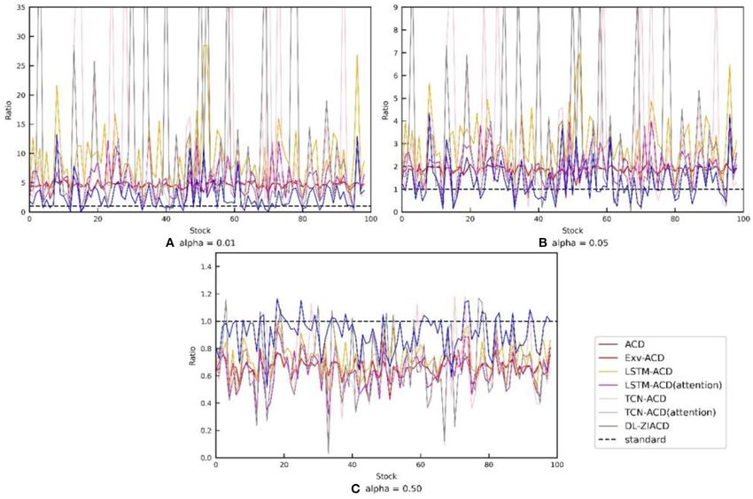
Shi et al.                                                                                                                A New Hybrid Duration Model

the linear equation of conditional mean duration to non-              RELATED WORK
linear cases. From the other perspective, the ACD family
models proposed in Refs. [7–11] try to choose a more suitable         ACD Family Models
distribution to characterize the uncertainty of the error term.       In order to estimate the conditional duration, the researchers
In 2018, a new ZIACD [12] model based on the zero-inflated            most use the autoregressive conditional duration (ACD) model
negative binomial distribution was proposed to address the            proposed by Engle et al. [2]. The classic version of the ACD model
problem of excessive zero values.                                     can be mathematically described as follows:
    Recently, financial researchers have paid more and more
                                                                                     yi = µi εi                                                  (1)
attention to machine learning methods, which succeed in
                                                                                                    p                 q
natural language processing (NLP) and computer vision                                             X                  X
                                                                                     µi = ω +            αj yi−j +         βh µi−h               (2)
(CV) tasks. Random forests (RF), support vector regression
                                                                                                   j=1               h=1
(SVR), and deep neural networks (DNN) are successively
applied to financial prediction tasks [13, 14]. Moreover, long                       εi ∼ Exp (1)                                                (3)
short-term memory (LSTM) networks were deployed for
constructing a hedge strategy in the financial market and             In Equation (1), duration yi is assumed as the multiplication
achieved the highest returns compared with benchmark models,          of the expectation µi and an error term εi . In Equation
including RF, DNN, and logistic regression classifier (LOG)           (2), the expectation µi is linearly dependent on the duration
[15]. Although, the machine learning methods mentioned                of the lagged periods and the lagged terms of itself. p and
above can forecast future expectation, in many situations,            q in Equation (2) represent orders of the lags, and the
we need to manage the risk of forecasting values (e.g., the           model defined by the above formulas can be labeled as ACD
financial volatility, the maximum loss given a probability            (p, q). Besides, exogenous variables can also be added as
level) simultaneously, which requires an accurate forecast            the
                                                                      Pr independent variables and are represented as the term
in conditional duration distribution. Consequently, various              l=1 γl xl in Equation (3). In this paper, the ACD (p, q)
studies [16–21] have been conducted to combine the machine            model with exogenous variables is written as Exv-ACD (p, q)
learning methods and classic statistical models to realize this       for short.
target. For instance, Peng et al. [20] used SVR to estimate                               p
                                                                                          X                 q
                                                                                                            X                  r
                                                                                                                               X
the mean and the volatility equations of a conventional                        µi = ω +         αj yi−j +         βh µi−h +          γl xl       (4)
GARCH model, and the proposed SVR-GARCH model                                             j=1               h=1                l=1
outperformed all the common models from the GARCH family
in volatility prediction.                                             Based on the work of Engle et al. [2], various studies were
    In this study, we extend the ZIACD model to establish             proposed to extend the classic ACD model by utilizing non-
a new hybrid model called “DL-ZIACD” for conditional                  linear functions to fit the conditional mean equation or choosing
duration distribution, utilizing a specially designed deep            more suitable distributions for the error term. Shi et al. [21]
learning (DL) network. The established hybrid DL-ZIACD                has reviewed the two types of extensions based on the classic
model is applied to nearly all constituent stocks of the              ACD model in detail. In a recent study, authors in Blasques
Chinese Shenzhen Stock Exchange 100 Index (SZSE 100),                 et al. [12] have utilized the zero-inflated negative binomial
and the results show that our DL-ZIACD model is superior              distribution [see Equation (5)] to address the excessive zero
to the benchmark models in forecasting conditional duration           values of duration yi and characterize the dynamics of the time-
distribution. The contributions of this paper can be summarized       varying location parameter with the general autoregressive score
as follows:                                                           (GAS) model.
(1) We propose a new hybrid zero-inflated duration model                       yi ∼ 0                        with probability π,
    by building a deep learning network to forecast the time-              yi ∼ NB (µi , α)                  with probability 1 − π.             (5)
    varying parameters of conditional duration distribution.
(2) The behavioral difference of large traders and small
    individual traders is taken into consideration when               Machine Learning Methods Applied to
    building the deep learning architecture of our
                                                                      Financial Data
    DL-ZIACD model.
                                                                      In recent years, more and more researchers have tried to
(3) The proposed model is applied to a large-scale dataset,
                                                                      capture the complexity of financial time series data, utilizing
    and fixed hyper parameters are adopted for all SZSE 100
                                                                      machine learning methods. Serjam and Sakurai [22] chose
    constituents to reduce the impact of manual tuning.
                                                                      the SVR model to predict the price movement in 1 min and
The remains of this paper are organized as follows: In section        got good results in simulated trading in the currency market.
Related Work, we review the related work of this paper. Section       Kumar and Thenmozhi [13] compare the performance of the
Methodology provides a detailed description of our proposed           linear discriminant analysis, logit, artificial neural network,
DL-ZIACD model. Section Empirical Research applied our                random forestand SVM in terms of predicting the direction of
proposed model to a large-scale dataset, and section Conclusion       stock index daily movement. Chong et al. [14] systematically
concludes this paper.                                                 analyzed the potential of deep neural networks for stock

Frontiers in Physics | www.frontiersin.org                        2                                           May 2021 | Volume 9 | Article 651528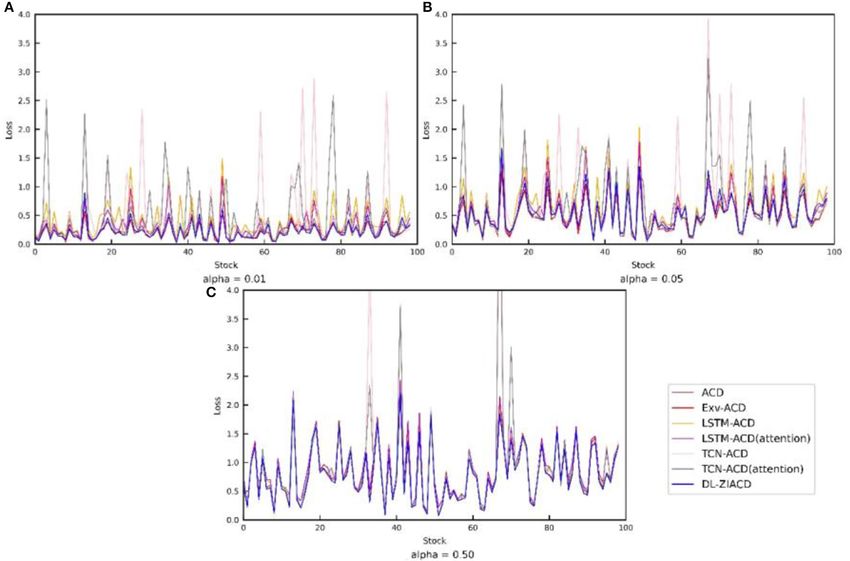
Shi et al.                                                                                                               A New Hybrid Duration Model

market prediction at high frequencies and found that the DNN            METHODOLOGY
method can extract additional information from the residuals
of the autoregressive model, not vice versa. In Fischer and             In this section, the process of establishing the DL-ZIACD model
Krauss [15], LSTM networks are employed to financial market             is described in two steps. First, we introduce a zero-inflated
predictions in order to recognize temporal information of               exponential distribution to address the problem of excessive
sequential data more effectively. However, these methods cannot         zero values for the duration with millisecond precision. Second,
assess the risk of the forecasted values. Therefore, the hybrid         a specially designed deep learning architecture is proposed
models combining machine methods and statistical models                 to predict the time-varying parameters of the zero-inflated
are proposed to realize this target while retaining the strong          exponential distribution.
fitting ability.
                                                                        Zero-Inflated Exponential Distribution
                                                                        When researchers analyze the ultrahigh frequency financial data,
Hybrid Models                                                           zero values account for a large proportion in the transaction
Many hybrid models have been proposed to forecast the future            duration even if the duration is recorded with precision of
state and assess the corresponding risk simultaneously. In              milliseconds. In the distributions used to describe the error
2003, Perez-Cruz et al. [16] utilized the SVM algorithm to              terms of the ACD family models, zero values usually have zero
give a better estimation for the parameters of the Generalized          density, and estimations problems may arise correspondingly
Autoregressive Conditional Heteroskedasticity (GARCH) model             [12]. Therefore, the zero-inflated negative binomial distribution
than the regular maximum likelihood method. In Refs. [17,               is utilized in Blasques et al. [12] to characterize the duration
18], the output of the GARCH model was added to the input               with excessive zeros. However, treating the duration with a count
variables of ANN to improve the volatility prediction of three          distribution is not a proper way if the transaction data are
stock exchange indexes and oil price, respectively. Following the       recorded with precision of milliseconds.
work of Refs. [17, 18], Kim and Won [19] used the parameters               In this study, we deal with the duration via zero-
of the multiple GARCH-type models and other explanatory                 inflated exponential distribution, which is a hybrid of one-
variables as the input of stacked LSTM layers to reduce                 point distribution and exponential distribution. The following
prediction errors. In Peng et al. [20], the mean and volatility         equation [Equations (6, 7)] describe the zero-inflated exponential
equations in the GARCH model are extended to the non-linear             distribution mathematically:
SVR decision function, and the proposed SVR-GARCH was
applied to the high frequency data of three cryptocurrencies                       yi ∼ 0                      with probability pi ,
and traditional currencies. Inspired by these works, Shi et al.                    yi ∼ E (λi )            with probability 1 − pi .              (6)
[21] extended the mean equation of the classic ACD model,
utilizing LSTM networks to propose the LSTM-ACD model. The                           P yi pi , λi ) = pi ,       yi = 0,
architecture of LSTM-ACD with the attention layer added is                           f yi pi , λi = 1 − p λe−λyi , yi > 0.                        (7)
abbreviated to LSTM-ACD (attention) in this paper. However,
the problem of excessive zero values is ignored in the work of
Shi et al. [21].                                                        For convenience, we introduce an indicator variable zi , defined as
   In the ZIACD model proposed by Blasques et al. [12],
a zero-inflated negative binomial distribution was chosen to                                              0,      yi > 0,
                                                                                               zi =
describe the discrete duration with excessive zeros. However,                                             1,      yi = 0.                         (8)
this model required the assumptions that the time-varying
location parameter followed the specification of GAS, and
other parameters were assumed to be static, which are                   Then the log likelihood function based on the distribution is
hard to fulfill in realistic situations. In a research for              calculated as follows:
assisting clinical decision-making, Kabeshova et al. [23] built                    n
a deep learning architecture based on zero-inflated mixture of                           ((1 − zi ) log((1 − pi )λi e−λi x ) + zi log(pi ))
                                                                                   X
                                                                              l=                                                                  (9)
multinomial distributions (ZiMM) to predict long-term and                          i=1
blurry relapses.
   In this paper, we also establish a hybrid model based                In this study, λi and pi are both supposed to be time-varying
on zero-inflated distribution to forecast conditional duration          parameters, which are dependent on the historical data. The
distribution. Compared with the ZIACD model proposed by                 dependency relationship will be characterized by a specially
Blasques et al. [12], we choose a zero-inflated exponential             designed deep learning architecture.
distribution as the underlying distribution because the research
data are recorded with millisecond precision. In addition,              The Proposed DL-ZIACD Model
the dynamics of the time-varying parameters of the zero-                There are two reasons that can explain the presence of excessive
inflated distribution is modeled by the specially designed              zero duration. One reason is that a large-volume trade may be
deep learning (DL) networks, which take the behavioral                  broken into several smaller trades and executed at the same
difference between large investors and small individual investors       time. The other reason for zero duration is that algorithmic
into consideration.                                                     traders, who can react instantly to the arbitrage opportunity

Frontiers in Physics | www.frontiersin.org                          3                                             May 2021 | Volume 9 | Article 651528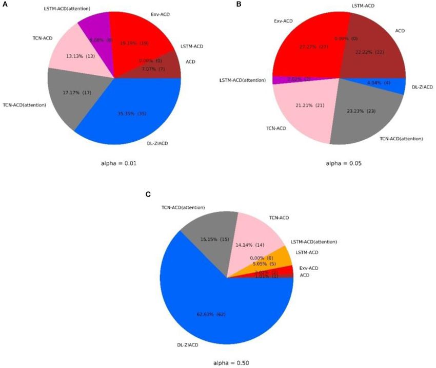
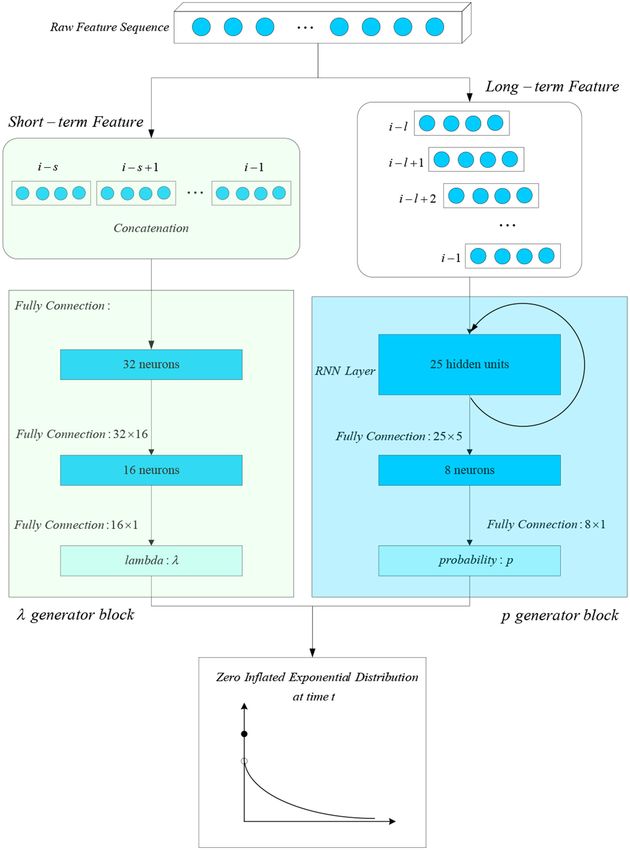
Shi et al.                                                    A New Hybrid Duration Model

  FIGURE 1 | Architecture of the DL-ZIACD model.

Frontiers in Physics | www.frontiersin.org         4   May 2021 | Volume 9 | Article 651528
Shi et al. A New Hybrid Duration Model
by the trading program. The orders with large volume are Algorithm 1
usually offered by large traders such as institutional traders, 1: Set the early stopping Patience = 5, learning rate ρ = .1, batch
and the algorithmic traders can also be viewed as a type of size K = 1000, Maximum Epochs = 100, Last Im provement =
institutional traders. Therefore, the probability of zero duration 0, Epoch = 0, −LLastBest = 0;
pi is highly related to the behavior of the large traders, who 2: Initialize weights Wp for the λ generator, Wλ for the p
can make a decision based on a long sequence of historical generator, and initialize the Adam Optimizer with an initial
data. Besides, a large-volume order means a high risk, which learning rate ρinitial = .1 and decay = .0001.
also drives the traders to spend more time on analyzing the 3: while not converged do
historical data. We take these factors into consideration and 4: i = 0
design a p generator block, consisting of a LSTM layer and a 5: while i · K < Ntrain do
fully connected layer to predict the probability of zero value 6: M = K
one step ahead. Contrastingly, the parameter λi is more likely 7: if(i − 1) · K ≥ Ntrain then M = Ntrain %K
decided by the behavioral pattern of small individual traders, 8: Get M new feature sequences Xp (1) , Xp (2) , ..., Xp (M) for
who provide the most liquidity for the stock market. Since the the p generator block,
small individual traders are much less professional than the large 9: Get M new feature vectors Xλ (1) , Xλ (2) , ..., Xλ (M) for the λ
traders, a two-layer fully connected network is utilized to predict generator block,
the λi parameter. 10: Get the corresponding M labels y(1) , y(2) , ..., y(M) and the
As shown in Figure 1, we feed a long-term feature to the current learning rate ρ from the Adam Optimizer,
p generator block and a short-term feature to the λ generator 11: Update the probability generator block:
block. We denote the raw feature sequence for the ith duration P −∂L(Xp (i) ,Xλ (i) ,y(i) )
Wp = Wp − ρ · Ki
as Fi : fj j = 1, 2, 3, · · · , i}, where, the fj represents the raw ∂Wp
feature vector of the jth transaction and consists the variables of 12: Update the lambda generator block:
P −∂L(Xp (i) ,Xλ (i) ,y(i) )
volume, duration, price, etc., The long-term feature is sequential Wλ = Wλ − ρ · Ki ∂Wλ
data of last l raw feature vectors selected from Fi . At the same 13: i = i + 1
time, we concatenate the last s raw feature vectors to get the 14: Calculate the negative log likelihood function −Lval on
short-term feature for the λ generator block. Then we can acquire validation set by Wλ and Wp
the distribution of the next duration based on the output of the 15: if −Lval < −LLastBest then
two blocks. −LLastBest = −Lval , Last Im provement = 0
We train the weights of the λ generator block and the p 16: else
generator block jointly. The objective function is the negative Last Im provement = Last Im provement + 1
value of the log likelihood function l, defined in Equation (9). 17: end if
In addition, the last 30% of the available data is selected as the 18: if Last Im provement ≥ Patience, then Break
test set. The remaining data are split into the training set and the 19: if Epoch ≥ MaximumEpochs, then Break
validation set according to the ratio of 7:3, and we make use of the 20: end while
early stopping method to prevent the overfitting problem. The
detailed training process of our DL-ZIACD model is presented in
Algorithm 1.
EMPIRICAL RESEARCH Evaluation Criteria
By training the parameters of the DL-ZIACD model based
Data on Algorithm 1, we can forecast the conditional duration
The widely quoted Shenzhen Stock Exchange 100 Index (SZSE ∧
distribution function g i for each transaction in the future and
100) is a weighted index of 100 leading companies with large ∧
market capitalization and good liquidity in the Chinese Shenzhen acquire the quantiles of g i . Being less likely to be affected by the
Stock Exchange market. The data sample used in our study cover extreme values of right-skewed distributions, the median (50%
all the constituents of the Shenzhen Stock Exchange 100 Index quantile) is chosen to predict the value of the next trade duration.
(SZSE 100) released on December 31st, 2016. For each stock, The prediction performance for the kth stock is measured
the first 100,000 transactions executed during the consecutive by mean absolute error (MAE), which can be calculated by
auction session in 2017 are selected for the experiment, and 30% Equation (10):
of the transactions are used as the test set. We exclude the stock of N
TIANJINZHONGHUAN SEMICONDUCTOR CO., LTD. from 1 X ∧
MAEkduration = y i − yi (10)
the data sample as this stock was suspended for all the year N
i=1
in 2017. Hence, the sample used in this study consists of 99
constituent stocks of SZSE 100 and has a data scale of 9,900,000 By averaging the MAE of the SZSE 100 constituent stocks, we get
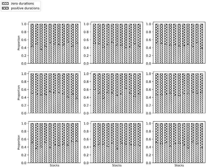
transactions. As shown in Figure 2, for most of the stocks studied, the MAEduration metric:
the proportion of zero duration exceeds 40%. Therefore, it is 99
theoretically inappropriate to ignore the problem of excessive duration 1 X
MAE = MAEkduration (11)
zero values. 99
k=1
Frontiers in Physics | www.frontiersin.org 5 May 2021 | Volume 9 | Article 651528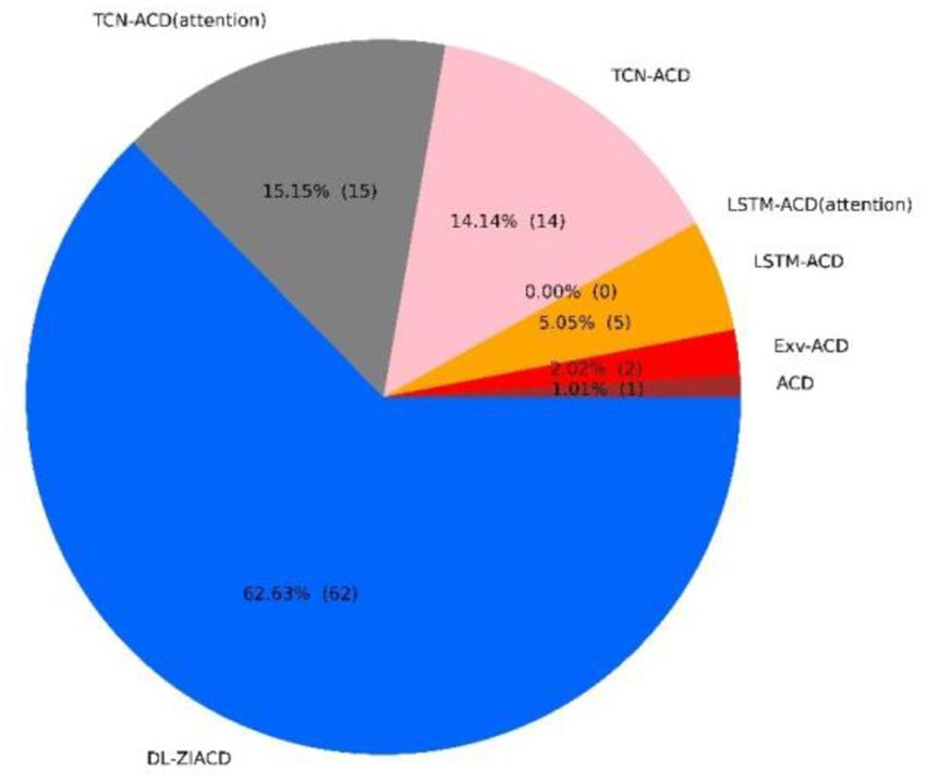
Shi et al.                                                                                                                                      A New Hybrid Duration Model

  FIGURE 2 | The proportion of zero duration and positive duration.

TABLE 1 | Overall performance of distribution forecasting.
                                        duration
                                  MAE                                           MAEratio
                                                                                   α                                                              QLα

                                                           α = 1%               α = 5%              α = 50%               α = 1%                α = 5%            α = 50%

ACD                                 1.67131                3.66832             0.87795               0.34317              0.21582               0.48578           0.83565
Exv-ACD                             1.67063                3.66256             0.87284               0.34286              0.21580               0.48505           0.83531
LSTM-ACD                            1.68613                7.73535             1.91049               0.27323              0.38412               0.65776           0.84306
LSTM-ACD (attention)                1.79279                4.23970             1.06065               0.36675              0.29881               0.59242           0.89639
TCN-ACD                             1.90891                8.54448             1.88053               0.35311              0.44006               0.71555           0.95446
TCN-ACD (attention)                 1.86040                9.73293             2.11968               0.34446              0.44071               0.70985           0.93020
DL-ZIACD                            1.58644                1.93162             0.68726               0.11907              0.21953               0.54281           0.79322

The bold value of each column means that the corresponding model achieves the best performance in this metric compared with other models.

To further measure the agreement between the forecasted                                    at the upper α level is denoted by Qα,i and defined by the
                 ∧                                                                         following equation:
distribution g i and the real distribution gi , we also evaluate
the prediction performance of quantiles at different probability
                             ∧
levels generated from g i . The quantile of the i-th trade duration                                                   α = P yi < Qα,i                                 (12)

Frontiers in Physics | www.frontiersin.org                                            6                                                May 2021 | Volume 9 | Article 651528
Shi et al. A New Hybrid Duration Model
Then the violation rates (VR) [11] can be given by
N
∧ 1 X
α= I yi > Qα,i (13)
N
i=1
where I represents an indicator function, which takes value 1
when duration yi exceeds the quantile Qα,i and takes value 0 in
∧ ∧
other cases. We calculate the ratio of α to α by Rα = α/α.
The closer Rα is to 1, the better the performance is. As shown
in Equation (14), the MAEαratio metric is used to summarize the
quantile forecasting performance on the 99 constituents of SZSE
∧
100, where Rα,k denotes the α/α for the kth stock.
99
1 X
MAEαratio = Rα,k − 1 (14)
99
k=1
FIGURE 3 | Detailed comparison of the seven models in MAE duration by a pie
chart [the size of each pie slice represents the percentage (number) of stocks
In addition, the loss function QL defined in Koenker and Bassett
on which the corresponding model achieves the lowest MAE duration ]. [24] to evaluate the performance of quantile regression is also
chosen to assess the quantile forecasting performance in this
∧
FIGURE 4 | Detailed comparison of the 7 models in Rα = α/α by a line chart. (Each full line is plotted by connecting the Rα value from the corresponding model on
each stock, while each black dotted line is a horizontal line at 1 value).
Frontiers in Physics | www.frontiersin.org 7 May 2021 | Volume 9 | Article 651528Shi et al. A New Hybrid Duration Model
paper. The quantile loss function for each stock can be calculated (1, 1), (1, 2), (2, 1), and (2, 2) for each stock according
as follows: to Akaike information criterion (AIC) [26]. As the temporal
convolutional network (TCN) [25] architecture has exhibited
N
X superiority over the recurrent architectures in many sequence
QLα = yi − Qα,i (1 − α) − I yi < Qα,i (15) modeling tasks, we can also extend the mean equation of
i=1
the classic ACD model by TCN architecture to propose a
TCN-ACD model. In addition, the attention layer can also be
Similar to the MAEratio metric, we also average the QLα of the
added to the TCN-ACD to establish a TCN-ACD (attention)
SZSE 100 constituent stocks to acquire the QLα , which reflects
model. We set a number of filters to 16, dilation to [2,
the overall performance of quantile forecasting.
3, 5, 9], and kernel size to 2. In this paper, the ACD,
Performance Exv-ACD, LSTM-ACD, LSTM-ACD (attention), TCN-ACD,
In section Related Work, the ACD, Exv-ACD, LSTM-ACD, and TCN-ACD (attention) models are chosen as the benchmark
LSTM-ACD (attention) model have been introduced. In this models. The empirical results of the models are summarized
paper, trade volume is specified as the exogenous variable for in Table 1.
the Exv-ACD model. In the application of the ACD model As shown in Table 1, our proposed DL-ZIACD model clearly
duration
and the Exv-ACD model, we choose the best order from outperforms all the other models in MAE , which exhibits
FIGURE 5 | Detailed comparison of the seven models in QLα by a pie chart [the size of each pie slice represents the percentage (number) of stocks on which the
corresponding model achieves the lowest QLα ].
Frontiers in Physics | www.frontiersin.org 8 May 2021 | Volume 9 | Article 651528Shi et al. A New Hybrid Duration Model
the superiority of the DL-ZIACD model over forecasting the We apply the DL-ZIACD model, as well as the benchmark
center location of conditional duration distribution. Because models, to a large dataset, including all the constituents of SZSE
duration
MAE is the average value of 99 MAE, we count the 100 with a data scale of 9,900,000 transactions. Meanwhile,
number of stocks on which the DL-ZIACD performs best. As fixed hyper parameters are chosen for all the stocks to
can be seen in the following Figure 3, the DL-ZIACD is superior reduce the effect of manual tuning. Empirical results show
to the other six models on more than 60 of the SZSE 100 that the DL-ZIACD model can provide accurate and robust
constituents, which validates the robustness of DL-ZIACD. The forecasts in both central location and extreme quantiles for
TCN-ACD (attention) model places second and achieves the the conditional duration distribution. From the perspective
lowest MAEduration on 15 stocks. of overall performance, the DL-ZIACD achieves the best
In terms of metric MAEαratio , the DL-ZIACD model also results in most of the overall metrics (e.g., MAE1% ratio ). In
exhibits the best performance at all three α levels. From addition, the DL-ZIACD model outperforms all the benchmark
Figure 4, we can see that the Rα lines (blue color) of DL-ZIACD models on most of the constituent stocks in MAEduration
are also apparently closer to the horizontal line at 1 value, and Rα at all probability levels. That means a high degree
compared with other lines in all subfigures. This indicates the of agreement between the forecasted distribution and the
excellent and robust performance of our DL-ZIACD model in real distribution.
quantile forecasting. The scope of using our DL-ZIACD model is not limited to
The QLα is another type of a metric for evaluating analyze the financial transaction duration. The proposed DL-
quantile forecasting performance. We can see from Table 1 ZIACD model can also be utilized to study the inter-times of
that DL-ZIACD achieves the lowest QL when α = 50%, arriving of queueing system. In this study, the historical data of
places third when α = 1%, and when α = 5%. From fixed length are fed to the λ generator block of the deep learning
Figure 5, we can find that DL-ZIACD achieves the lowest architecture. For future research, it is possible to treat the length
QL on more stocks than all the other six models, when of the historical data as a parameter to improve the generalization
α = 1% and 50%. From Figure A1 in the Appendix ability of the model.
part, we also find that DL-ZIACD provides a robust quantile
forecasting result as no extreme large QLvalues appear in DATA AVAILABILITY STATEMENT
the application of the DL-ZIACD model. Therefore, the DL-
ZIACD model can provide accurate forecasts in both central Publicly available datasets were analyzed in this study. The
location and extreme quantiles, which validates the agreement datasets analyzed for this study can be purchased from Shanghai
between the forecasted conditional duration distribution and the Wind Information Co., Ltd. (https://www.wind.com.cn/).
real distribution.
AUTHOR CONTRIBUTIONS
CONCLUSION
YS: resources, supervision, and funding acquisition. WD:
In this paper, a DL-ZIACD model is established to forecast the formal analysis, software, visualization, and writing -
conditional distribution for financial transaction duration. The original draft. WL: conceptualization, methodology,
problem of excessive zero duration is addressed by the zero- and writing - review & editing, and validation. All
inflated exponential distribution, the time-varying parameters authors have read and agreed to the published version of
of which are forecasted by a specially designed deep learning the manuscript.
architecture that takes the behavioral differences between the
large traders and the small individual traders into consideration. FUNDING
The proposed DL-ZIACD model is able to utilize the strong
fitting ability of deep learning methods while retaining the ability This work was supported by National Natural Science
of providing a probabilistic output. Foundation of China (Nos. 71771204 and 71932008).
REFERENCES 5. Bauwens L, Giot P. Asymmetric ACD models: introducing
price information in ACD models. Empir Econ. (2003) 28:709–
1. Moallemi CC, Yuan K. A Model for Queue Position Valuation in a Limit Order 31. doi: 10.1007/s00181-003-0155-7
Book. SSRN. (2016) doi: 10.2139/ssrn.2996221 6. Meitz M, Teräsvirta T. Evaluating models of autoregressive
2. Engle RF, Russell JR. Autoregressive conditional duration: a new model conditional duration. J Bus Econ Stat. (2006) 24:104–
for irregularly spaced transaction data. Econometrica. (1998) 66:1127– 24. doi: 10.1198/073500105000000081
62. doi: 10.2307/2999632 7. Lunde A. A Generalized Gamma Autoregressive Conditional Duration
3. Bauwens L, Giot P. The logarithmic ACD model: an application to the Model. ResearchGate. (1999) Available online at: https://www.researchgate.
bid-ask quote process of three NYSE stocks. Ann DÉconomie Stat. (2000) net/publication/228464216 (accessed July 30, 2020).
60:117–49. doi: 10.2307/20076257 8. Hautsch N. The Generalized F ACD Model. Mimeo: University of
4. Zhang MY, Russell JR, Tsay RS. A non-linear autoregressive conditional Konstanz. (2001).
duration model with applications to financial transaction data. J Econom. 9. De Luca G, Gallo GM. Mixture processes for financial intradaily durations.
(2001) 104:179–207. doi: 10.1016/S0304-4076(01)00063-X Stud Nonlinear Dyn Econom. (2004) 8:1223. doi: 10.2202/1558-3708.1223
Frontiers in Physics | www.frontiersin.org 9 May 2021 | Volume 9 | Article 651528Shi et al. A New Hybrid Duration Model
10. De Luca G, Zuccolotto P. Regime-switching pareto distributions 20. Peng Y, Albuquerque PHM, Camboim de Sá JM, Padula AJA, Montenegro
for ACD models. Comput Stat Data Anal. (2006) 51:2179– MR. The best of two worlds: forecasting high frequency volatility for
91. doi: 10.1016/j.csda.2006.08.019 cryptocurrencies and traditional currencies with Support Vector Regression.
11. Yatigammana RP, Chan JSK, Gerlach RH. Forecasting trade durations via Expert Syst Appl. (2018) 97:177–92. doi: 10.1016/j.eswa.2017.12.004
ACD models with mixture distributions. Quant Finance. (2019) 19:2051– 21. Shi Y, Dai W, Long W, Li B. Improved ACD-based financial trade durations
67. doi: 10.1080/14697688.2019.1618896 prediction leveraging LSTM networks and attention mechanism. Math Prob
12. Blasques F, Holý V, Tomanová P. Zero-inflated autoregressive conditional Eng. (2021) 2021:7854512. doi: 10.1155/2021/7854512
duration model for discrete trade durations with excessive zeros. arXiv 22. Serjam C, Sakurai A. Analyzing performance of high frequency currency
[Preprint]. (2018). doi: 10.2139/ssrn.3314218 rates prediction model using linear kernel SVR on historical data. In: Asian
13. Kumar M, Thenmozhi M. Forecasting Stock Index Movement: A Comparison Conference on Intelligent Information and Database Systems. Kanazawa:
of Support Vector Machines and Random Forest. ResearchGate (2006) Springer (2017). p. 498–507. doi: 10.1007/978-3-319-54472-4_47
Available online at: https://www.researchgate.net/publication/228265807 23. Kabeshova A, Yu Y, Lukacs B, Bacry E, Gaïffas S. ZiMM: a deep learning model
(accessed November 15, 2020). for long term and blurry relapses with non-clinical claims data. J Biomed
14. Chong E, Han C, Park FC. Deep learning networks for stock market analysis Inform. (2020) 110:103531. doi: 10.1016/j.jbi.2020.103531
and prediction: methodology, data representations, case studies. Expert Syst 24. Koenker, R, Bassett, G. Regression quantiles. Econometrica. (1978) 46:33–
Appl. (2017) 83:187–205. doi: 10.1016/j.eswa.2017.04.030 50. doi: 10.2307/1913643
15. Fischer T, Krauss C. Deep learning with long short-term memory 25. Bai S, Zico Kolter J, Koltun V. An empirical evaluation of generic
networks for financial market predictions. Eur J Oper Res. (2018) 270:654– convolutional and recurrent networks for sequence modeling. arXiv
69. doi: 10.1016/j.ejor.2017.11.054 [Preprint]. (2018).
16. Pérez-cruz F, Afonso-rodríguez JA, Giner J. Estimating GARCH 26. Akaike H. Information Theory and an Extension of the Maximum Likelihood
models using support vector machines. Quant Finance. (2003) Principle Budapest. (1998). doi: 10.1007/978-1-4612-1694-0_15
3:163–72. doi: 10.1088/1469-7688/3/3/302
17. Kristjanpoller W, Fadic A, Minutolo MC. Volatility forecast using Conflict of Interest: The authors declare that the research was conducted in the
hybrid Neural Network models. Expert Syst Appl. (2014) 41:2437– absence of any commercial or financial relationships that could be construed as a
42. doi: 10.1016/j.eswa.2013.09.043 potential conflict of interest.
18. Kristjanpoller W, Minutolo MC. Forecasting volatility of oil price using an
artificial neural network-GARCH model. Expert Syst Appl. (2016) 65:233– Copyright © 2021 Shi, Dai and Long. This is an open-access article distributed
41. doi: 10.1016/j.eswa.2016.08.045 under the terms of the Creative Commons Attribution License (CC BY). The use,
19. Kim HY, Won HC. Forecasting the volatility of stock price index: distribution or reproduction in other forums is permitted, provided the original
a hybrid model integrating lstm with multiple garch-type models. author(s) and the copyright owner(s) are credited and that the original publication
Expert Syst Appl. (2018) 103:25–37. doi: 10.1016/j.eswa.2018. in this journal is cited, in accordance with accepted academic practice. No use,
03.002 distribution or reproduction is permitted which does not comply with these terms.
Frontiers in Physics | www.frontiersin.org 10 May 2021 | Volume 9 | Article 651528Shi et al. A New Hybrid Duration Model APPENDIX FIGURE A1 | Detailed comparison of the seven models in QLα by a line chart. (Each full line is plotted by connecting the QLα value from the corresponding model on each stock). Frontiers in Physics | www.frontiersin.org 11 May 2021 | Volume 9 | Article 651528
You can also read