A Neural Network-Based Sustainable Data Dissemination through Public Transportation for Smart Cities
←
→
Page content transcription
If your browser does not render page correctly, please read the page content below
sustainability

Article
A Neural Network-Based Sustainable Data
Dissemination through Public Transportation
for Smart Cities
Rashmi Munjal *, William Liu, Xue Jun Li *                and Jairo Gutierrez
 School of Engineering, Computer, and Mathematical Sciences, Auckland University of Technology,
 Auckland 1010, New Zealand; william.liu@aut.ac.nz (W.L.); jairo.gutierrez@aut.ac.nz (J.G.)
 * Correspondence: rashmi.munjal@aut.ac.nz (R.M.); xuejun.li@aut.ac.nz (X.J.L.)

 Received: 15 October 2020; Accepted: 3 December 2020; Published: 10 December 2020

 Abstract: In recent years, there has been a big data revolution in smart cities dues to multiple
 disciplines such as smart healthcare, smart transportation, and smart community. However, most
 services in these areas of smart cities have become data-driven, thus generating big data that require
 sharing, storing, processing, and analysis, which ultimately consumes massive amounts of energy.
 The accumulation process of these data from different areas of a smart city is a challenging issue.
 Therefore, researchers have started aiming at the Internet of vehicles (IoV), in which smart vehicles are
 equipped with computing and storage capabilities to communicate with surrounding infrastructure.
 In this paper, we propose a subcategory of IoV as the Internet of buses (IoB), where public buses
 enable a service as a data carrier in a smart city by introducing a neural network-based sustainable
 data dissemination system (NESUDA), where opportunistic sensing comprises delay-tolerant data
 collection, processing and disseminating from one place to another place around the city. The objective
 was to use public transport to carry data from one place to another and to reduce the traffic from
 traditional networks and energy consumption. An advanced neural network (NN) algorithm was
 applied to locate the realistic arrival time of public buses for data allocation. We used the Auckland
 transport (AT) buses data set from the transport agency to validate our model for the level of accuracy
 in predicted bus arrival time and scheduled arrival time to disseminate data using bus services.
 Data were uploaded onto buses as per their dwelling time at each stop and terminals within the
 coverage area of deployed RSU. The offloading capacity of our proposed data dissemination system
 showed that it could be utilized to effectively complement traditional data networks. Moreover,
 the maximum offloading capacity at each parent stop could reach up to 360 GB with a huge saving of
 energy consumption.

 Keywords: big data; data scheduling; delay tolerant network (DTN); bus arrival time; public transport;
 bus dwell time; neural network

1. Introduction
     Nowadays, a huge surge in Internet traffic raises many concerns over the capacity of the
infrastructure. All the mobile devices are equipped with wireless network interfaces and which
introduce new demands in the wireless network leading to the digital society with the emerging
trend of “big data” with features of high-volume, high-velocity, and high-variety. With a limited
spectrum of resources, mobile operators may be struggling to provide adequate bandwidth to handle
the amount of traffic generated by their users. These big data sources in a smart city are posing
sustainability challenges to achieve ecosystem balance and, at the same time, perform the day-to-day
data transmission activities. Therefore, recently, much attention has been focused on accommodating

Sustainability 2020, 12, 10327; doi:10.3390/su122410327                         www.mdpi.com/journal/sustainability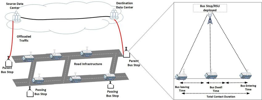
Sustainability 2020, 12, 10327                                                                      2 of 26

big data needs by leveraging the traffic burden from the traditional network to other networks, which
is also known as data offloading. This technique helps to reduce the congestion over the conventional
network and make bandwidth available for other users for effective usage. The Cisco visual networking
index (VNI) [1] has revealed that fixed networks have been used to offload data from mobile data
in 2019, and it was approximately 51% of total global traffic. Therefore, it is possible to offload data
from the network to another available network as per the user’s preferences. Similarly, we also
require an alternative approach to alleviate this pressure on the existing infrastructure. Thus, efficient
data dissemination mechanisms considering the urban Internet bandwidth consumption should be
designed. We consider in addition to the traditional network to shift traffic and improve bandwidth
utilization. Therefore, Wi-Fi enabled and on-board unit (OBU) equipped buses and bus stops show the
potential for forming the communication backbone. The main aim is to utilize public transport buses
to carry data from one place to another place on their predefined route. Our public transport system
exploits nearby communications, short-term storage at bus stops, and predictable bus movement
to deliver non-real-time information. We used the public transport network due to their scheduled
movement and fixed timetable. However, we noticed a delay in bus arrival time in real-life due to
some uncertainties. Therefore, we applied an ANN algorithm to have more realistic information on
bus arrival time at each bus stop. To validate our idea, we used Auckland Transport (AT) historical
data to analyze bus daily movement patterns and applied an advanced neural network algorithm to
understand the variance between predicted arrival time and schedule travel time for more realistic
information to authenticate that public transport can be used as an energy-efficient communication
channel. All public vehicles stop at bus stops for a long or short duration known as bus dwell time
during their fixed travel route, and data were uploaded and downloaded at these bus stops only.
It was important to be within the range of the interfaces for better and fast communication between
bus stops and buses. We utilized the bus arrival time, departure time, and speed of all public buses
to load and offload the data. However, there were some factors such as signals, traffic fluctuations,
peak hours, and road incidents, which often lead to delay in set schedules and results in irregularities
in journey times and bus arrival times. Many other factors are available that lead to the variation of
public bus travel times, and some of these factors were not measurable. Unexpected delays could be
predicted. However, we emphasize more on historical data provided by the transport agency and
carry out analysis to get the most accurate prediction results. The main contributions of this paper are
the following:

1.     We obtained the characterizations of the public transport bus systems that currently exist and
       determined bus daily movement patterns to form a data transmission network named as neural
       network-based sustainable data dissemination system (NESUDA).
2.     We applied the advanced neural network algorithm to analyze the arrival time based on historical
       data. We analyzed the difference between scheduled and predicted arrival times to estimate the
       accuracy of utilizing public buses for data dissemination. The Auckland transport data set was
       used to validate our model.
3.     We proposed a data dissemination algorithm using data scheduling onto buses as per their dwell
       time at each passing stop and stopping stop.
4.     For evaluation, a detailed comparative analysis of energy consumption is performed for traditional
       and vehicular networks.

      The remainder of the paper is structured as follows: in Section 2, we present the literature on
existing work done on utilizing public transport for carrying delay-tolerant data and their arrival
predictions. In Section 3, we develop our data dissemination system using existing road infrastructure
utilizing their scheduled movement and their arrival predictions with the help of the advanced neural
network (ANN) algorithm. Section 4 helps us to validate the road network capacity of Auckland
Transport and estimate the accuracy of predicted and actual arrival time of buses for the allocation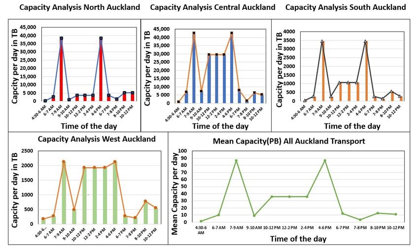
Sustainability 2020, 12, 10327                                                                        3 of 26

of data in addition energy consumption analysis. Section 5 concludes this paper with directions for
future work.

2. Related Work
      A huge range of wireless devices and data generated from these devices are incurring a fast
escalation of both network bandwidth and energy demands. However, it is very challenging to attain
a high-level quality of collective services and energy-efficient wireless networking in this big data
era [2,3]. Therefore, one of the research community’s main aims is to maximize the performance of the
communication system in an energy-efficient manner [4–6]. For example, a significant surge in Internet
traffic has raised many concerns over the strength of the infrastructure that keeps things running [7].
Accommodating this evolution requires an alternative approach [8] to alleviate this pressure on existing
infrastructure. Many researchers started exploring the Internet of Vehicles (IoV) [9–11] as a data mule
to deliver data from different places. Many cooperative approaches have been proposed for data
gathering from different locations [12]. Another paper discussed the suitable logical links to transfer
data in bulk using vehicles [13]. In this approach, the author plots an overlay network over an existing
network, and all the moving nodes act as relay nodes. The results proved that a huge amount of
data could be transmitted using road infrastructure. In summary, data offloading strategies [14] were
reported in the literature to transfer huge amounts of data onto vehicles. The authors in paper [15]
performed a study on 3G data offloading through a Wi-Fi network. They have discussed on-the-spot
offloading and delayed offloading with results on offloading efficiency for different traffic intensity, file
size distributions, and delay the deadline. Paper [16] also discussed on-spot offloading for the available
network in the heterogeneous networks in terms of offloading efficiency and delay. Rosamaria et al. [17]
introduced an architecture for convenient parking management in smart cities using intelligent parking
assistants to attain sustainable urban mobility. IPA hardware informs drivers about the availability of
a parking stall and allows them to reserve it. Paper [18] used spatiotemporal features of the Xingtai
bus company dataset and then combined two prediction models, a long short-term memory (LSTM)
and artificial neural networks (ANN) comprehensive prediction model for bus arrival time prediction.
The ANN outperforms the results in accuracy and travel time prediction.
      The existing data dissemination schemes using vehicles, such as [19–23], are primarily based on
the opportunistic transfer of bulk data. Komnios et al. [24] focused on metropolitan environments
intending to provide delay tolerant services to those areas where end-to-end connectivity is not
possible. It utilizes the CARPOOL plan to connect between ferries and gateways to compute routes
for online gateways. Therefore, free public Internet access, Wi-Fi hot spots and their connections
were setup through public transport such as ferries, buses, and trams. DTN gateways are in offline
mode near all ferries’ stops to get an Internet request from all end-users and in such a way act
as a relay node. With prior knowledge of contacts between gateways, a high delivery ratio with
minimum overhead has been achieved. For heterogeneous networks and to connect parked vehicles to
the Internet, Bendouda et al. [25] proposed a programmable architecture called a software-defined
vehicular network based on connected dominating sets of vehicles. In another piece of work [26], the
author proposed a code transportation technique to transmit data all over a smart city. When any of the
moving vehicles enter the range of deployed sensors, sensors synchronize their pushed code with the
cloud center and start transmission onto the vehicle with a data mule. The author [27] used taxis and
buses as a data carrier and validated the model using a large data set in Rio de Janeiro, Brazil. Yilong
et al. [28] also introduced collaborative content delivery using a group of vehicles to cooperate with
RSU for data dissemination. Naseer et al. [29–31] also proposed a data dissemination scheme using a
moving vehicle for data accumulation and delivery. The strategy also used conventional networks and
moving vehicles based upon their trajectories to collect data with delay tolerance to send from one
place to another. A comparison illustrates that energy cost is less in a vehicular network in comparison
with cellular networks. In our previous work [32–34], we have already defined software-defined
connectivity to disseminate data using public transport networks. The controller takes all forwarding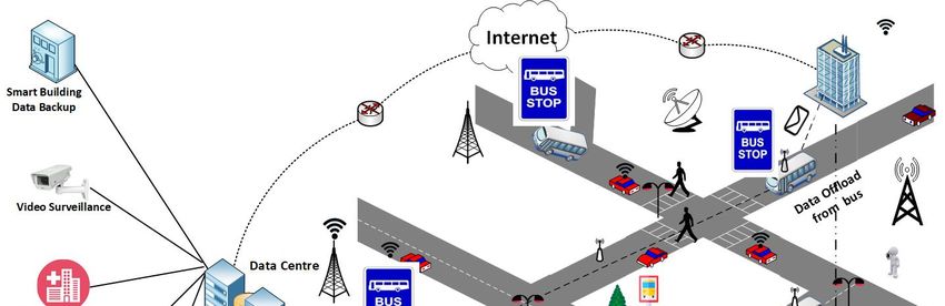
Sustainability 2020, 12, 10327                                                                      4 of 26

decisions based upon user’s profiles and their preferences. In such a way, there is a huge saving of
energy to send data using the existing road network. However, for large-scale data transfers, such
schemes can lead to better results if the bus’s accurate time for arrival is known in advance for data
offloading onto public transport vehicles.
     Furthermore, many researchers have already addressed the bus arrival time prediction problem
for many other reasons. Major techniques brought in to practice for predicting arrival time were
historical based models, regression models, Kalman filter-based models, and machine learning models.
Manasseh and Sengupta [35] used the concept of machine learning to predict the driver’s destination.
They used a data set of the San Francisco Bay Area for about 2–9 weeks and achieved 97% accuracy.
For example, Patnaik et al. [36] predicted bus arrival time with a set of multiple linear regression
models applying a set of features such as boarding and landing passengers, distance, several bus stops,
dwell times, and weather descriptors as independent variables. One of the recent studies [37], which
concentrates on finding nonlinear relationships between the independent variable and dependent
variables to handle complicated and noise data using ANN model-based approaches. In such a way,
they predict bus arrival time prediction of different bus routes for accurate measurement. The authors
in paper [38] introduced a deep learning-based mobile data offloading model using mobile edge
computing. They offloaded data onto vehicles based upon prediction value, priority, and cross-entropy
method. Zhang et al. [39] proposed a data-driven approach for predicting bus travel time, and using
those prediction results in traffic flow theory. These data-driven approaches predict future travel time
by using large databases and their empirical relationships, excluding the physical behaviors of the
trained system. Recent studies on bus arrival time predictions reveal that the ANN model is best
known for its accuracy and robustness [40]. In addition to it, Mahdi et al. [41] proposed an offloading
strategy for railway data centers to offload huge amounts of stored non-critical data. The data gets
offloaded when the train enters and keeps on offloading until it leaves the train station and remains
in coverage. Therefore, all existing work motivates the development of a novel system model for
an energy-efficient network with a reasonable amount of data offloading onto buses. In this paper,
we propose a neural network-based data dissemination architecture for initiating our data transfer
with bus arrival time prediction for accurate modeling of data allocation onto buses.

3. System Model

3.1. Neural Network-Based Sustainable Data Dissemination System (NESUDA)
      The proposed framework depicts a neural network-based sustainable data dissemination system
(NESUDA) as shown in Figure 1 for large-scale data transfer using a set of buses as a data carrier to be
picked up at each bus stop. Our system consists of a central controller (CC), data center (DC), roadside
units (RSU) deployed at the bus stop, and buses. The traditional way is to use a traditional network to
handle this data. However, this alternative communication channel layer of public transport networks
can be used for large-scale data transfer accumulated at each data center using a set of buses and data
picked up at each bus stop. This channel is being technologically advanced from DTN working on the
paradigm of store-carry-forward. The generated data are accumulated at the data center near bus stops.
The central controller takes all decisions to upload data onto selected buses as per bus route. Our model
takes advantage of the existing public transport network for data dissemination. These buses can be
utilized efficiently for delay-tolerant data transmission. The central controller takes all decisions to
upload data onto selected buses as per bus route. All public transport vehicles are equipped with
removable storage devices and on-board units. Moving further, the collection of data is at all bus stops
where buses stop for a long or short duration during their travel route and data are uploaded onto
buses and downloaded on these parking spots only at the other end. It is important to be into the
range of interface for better and fast communication between bus stops and buses. The network used
for communication is periodic and predictable as per the scheduled timetable. The most significant
part of the data dissemination system is the accuracy in bus arrival time for allocating data as per their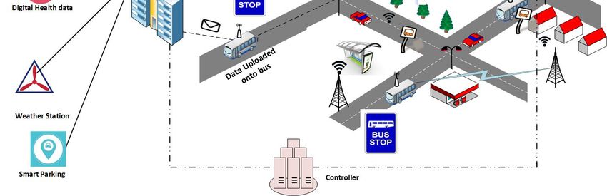
Sustainability 2020, 12, 10327 5 of 26
arrival and dwell time at each bus stop. Therefore, we implement an advanced neural network for
Sustainability
predicting 2020, 12, xtime
arrival FOR for
PEER REVIEW
more realistic
arrival time information for data transfer. 5 of 25
Figure 1.
Figure Neuralnetwork-based
1. Neural network-based sustainable
sustainable data
data dissemination
dissemination system
system (NESUDA).
(NESUDA).
3.2. Bus Arrival Time Prediction Model
3.2. Bus Arrival Time Prediction Model
In the proposed system, we allocate data onto buses at each bus stop. The performance of data
In the highly
allocation proposed system,
depends we allocate
upon coverage,data onto buses
mobility, andatduration.
each bus Forstop.accurate
The performance
modeling of of data
data
allocation highly depends upon coverage, mobility, and duration. For accurate modeling of data
allocation, it is mandatory to know the accurate arrival time, leaving time, and dwell time of the bus at
allocation, it is mandatory to know the accurate arrival time, leaving time, and dwell time of the bus
each bus stop. Thus, machine learning techniques are applied to develop a bus arrival time prediction
at each bus stop. Thus, machine learning techniques are applied to develop a bus arrival time
model to give precise bus arrival information for applying proactive strategies for data dissemination.
prediction model to give precise bus arrival information for applying proactive strategies for data
The provision of time and accuracy is important information for data allocation onto these buses for
dissemination. The provision of time and accuracy is important information for data allocation onto
successful data transmission. The accurate information helps the controller to make a forwarding
these buses for successful data transmission. The accurate information helps the controller to make a
decision based upon the source and destination location and the route of the bus. An advanced neural
forwarding decision based upon the source and destination location and the route of the bus. An
network model is adopted using input features such as bus stops, bus routes, trips and many other
advanced neural network model is adopted using input features such as bus stops, bus routes, trips
features of a transport agency. Figure 2 shows the architectural diagram of the ANN algorithm w.
and many other features of a transport agency. Figure 2 shows the architectural diagram of the ANN
It encompasses three layers, i.e., an input layer, a hidden layer, and an output layer.
algorithm w. It encompasses three layers, i.e., an input layer, a hidden layer, and an output layer.
1. Input layer: This layer provides input to the neural network such as bus route, trips, and its
1. Input layer: This
corresponding layer provides
metadata. The businput
route to the neural
consists network
of its name, id, such as busname.
and agency route, The
trips,
busand
tripitsis
corresponding
characterized by metadata. The bus route
shape coordinates, tripconsists
id, routeofid,itsand
name, id, andThe
direction. agency name.
first and lastThe
busbus
stoptrip
of
iseach
characterized
route is theby shapeand
source coordinates,
destinationtrip id,respectively.
stop, route id, andThe direction. The interacts
input layer first and with
last bus
the stop
data
of
provided, accepts data in the form of signals or features. These features are then normalizedthe
each route is the source and destination stop, respectively. The input layer interacts with to
data provided,
achieve accepts data
better numerical in the form
precision whenofasignals or features.
mathematical modelThese features
is applied are hidden
at the then normalized
layer [42].
to
Atachieve better
this stage, numerical
small random precision
values arewhen a mathematical
initialized model
to the weights. Theisinput
applied
layerat just
the hidden
passes onlayer
the
[42]. At this stage,
information to thesmall
hiddenrandom values
layer after are initialized
adding to the weights.
weights without The input layer
any computation. just passes
It is represented
on the information
below. (Table 1) to the hidden layer after adding weights without any computation. It is
represented below. (Table 1) Xi = θ(X1 , X2 , ..., Xn ) (1)
Xi = θ(X 1 , X2,...Xn) (1)
Sustainability 2020, 12, 10327                                                                                 6 of 26

2.     Hidden layer: This layer accepts all the information from the input layer and feed-forward to
       all hidden layers to process it and forward it to the output layer. Next, this layer extracts all
       the features from the input layer and performs processing or training of the network with an
       activation function. The main motive of the activation function is to add nonlinearity into the
       network. There are many activation functions such as sigmoid, logistic, and hyperbolic tangent
       functions (tanh), ReLU, are the most common choices. In our model, the ReLU function is used as
       a rectifier unit for all input values and direct to (0, θ). This function is given by

                                                    f (θ) = max(0, θ)                                             (2)

       Here, the function outputs zero if the input values in the nonlinear function are negative or else
       equal to the value gives as input.
3.     Output layer: The output layer consists of results generated from previous layers. It updates
       errors as well as the weights associated with the connections (edges). The number of neurons in
       this layer corresponds to the output values of the problem. The neuron with n inputs calculates
       its output, as shown in Equation (3). As discussed above, all the input features are feed-forward,
       and then some bias weight is applied to the hidden layer, and finally, the output layer process the
       desired variables to be predicted.
                                                     Xn
                                              a = f(    Wi Xi + b)                                      (3)
                                                          i=1

       where Xi is the ith input Wi is the value of ith weight b is the bias, and f is an activation function.
4.     Training, testing, and validation: Although the basic procedure of training any neural network
       is the same, however, the accuracy of the outcome relies on the features of input or output
       combinations. Therefore, it is highly important to validate a network to verify that training
       accuracy is sufficient or more iterations are required. During our ANN training algorithm as
       shown in Figure 3, we separate data input into two categories: one part is used to define the
Sustainability 2020, 12, x FOR PEER REVIEW                                                                    7 of 25
       model, and the other part is used to validate the model. We use transport network input features
       asper
      as   per time,
                time, date,
                        date, stops,
                               stops, stop
                                       stoptime.
                                             time.Next,
                                                   Next,we
                                                         wesort this
                                                             sort    input
                                                                   this    data
                                                                        input    to feed-forward
                                                                               data               to the
                                                                                     to feed-forward   toinput  layer,
                                                                                                          the input
       the first
      layer,   the70%
                    firstof  data
                           70%  of can
                                   databe  considered
                                         can          as training
                                             be considered         data to
                                                            as training    construct
                                                                         data          the model,
                                                                              to construct        and the
                                                                                            the model, andnext   30%
                                                                                                            the next
       is used    for  testing  and  validation.
      30% is used for testing and validation.

          Figure 2. Bus arrival time prediction using an advanced neural network (ANN) architecture.
          Figure 2. Bus arrival time prediction using an advanced neural network (ANN) architecture.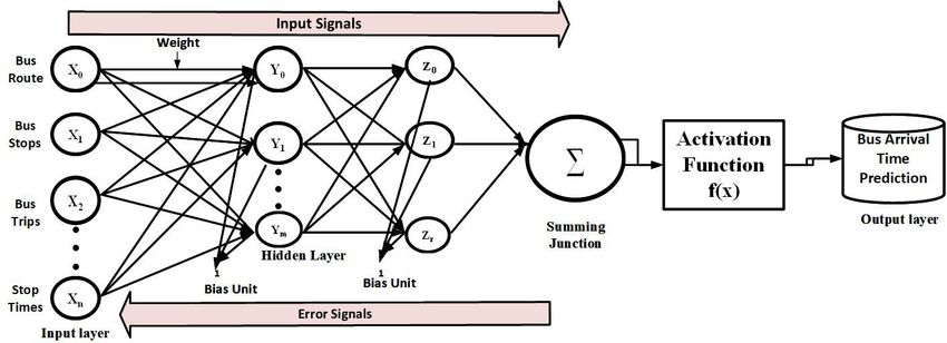
Sustainability 2020, 12, 10327                                                                          7 of 26
           Figure 2. Bus arrival time prediction using an advanced neural network (ANN) architecture.

                                       Figure 3.
                                       Figure    ANN model
                                              3. ANN model for
                                                            for the
                                                                 the public
                                                                     public transport
                                                                             transport network.
                                                                                       network.

                                           Table 1. Variables used in the proposed model.
    The steps below will be followed by our ANN model to predict arrival time:
    Step 1: GeneratingSymbol
                       observations of Meaning
                                        the bus route: A random observation of all trips is to be
generated and update zero
                      Xi  for bus stops whose  arrival time is to be predicted.
                                       Input variables
                                 Wi                    Weight
                                 f (θ)                 ReLU function
                                 s                     Speed of the bus
                                 tcd                   Contact duration
                                 ten                   Entering time
                                 tdw                   Dwell time
                                 tex                   Exit time
                                 d                     Distance between RSU and bus
                                 rsp(t)                Received signal strength
                                 dre f                 Reference distance
                                 Pr                    Received power
                                 σ                     Normal distribution random variable
                                 dex                   Distance after t seconds of bus leaving
                                 nb                    Background noise
                                 ρ                     Mac efficiency
                                 µ                     Throughput
                                 λmax                  Max data rate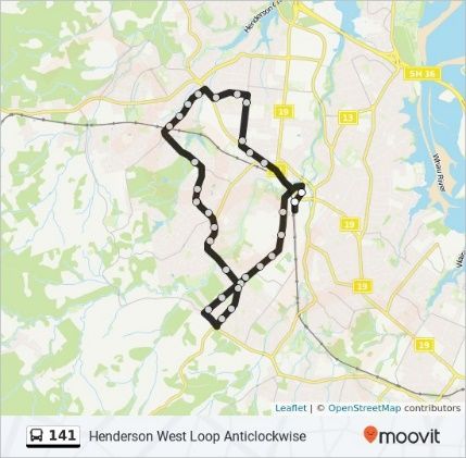
Sustainability 2020, 12, 10327                                                                        8 of 26

      The steps below will be followed by our ANN model to predict arrival time:
      Step 1: Generating observations of the bus route: A random observation of all trips is to be
generated and update zero for bus stops whose arrival time is to be predicted.
      Step 2: Retrieve bus stop location details of all bus routes: Next, following our algorithm, we will
fetch all the bus stops concerning their routes. For example, on the bus routes, there are a total of
29 bus stops. We will be calculating the bus arrival time for all these bus stops.
      Step 3: Generate a symbolic formula and perform ANN model training: Our ANN model is
accepting input as bus stop sequence (BS), the distance between two stops (d), the cumulative distance
for the whole test trip CDtt , the time between stops (Ts ), arrival time in seconds (ATs ), speed (S), and
cumulative travel time (CTTs ). Therefore, the initial symbolic formula description of the model to be
fitted will be as.
                                X = (Bs + ds + CDtt + Ts + ATs + S + CTTs )t                             (4)

      Step 4: Computing prediction and storing the predicted value: In the previous step, when a model
is trained with sample data of a fixed route, ANN model results are used to predict bus arrival time
for all other routes. These values will be stored in the predicted data frame and will be used for the
comparison between actual and predicted arrival time. Similarly, Step 3 and Step 4 will be repeated for
all the test trips.
      Step 5: Performance metrics evaluations: We will consider the following performance metrics to
estimate the results from the ANN model for all the predicted and actual arrival time values.

•     Mean absolute percentage error (MAPE) = MAPE is defined as the average percentage difference
      between the observed value and the predicted value of bus arrival time. Where yi = Predicted
      value, y0 = observed value.
                                                 n
                                             1 X yi − y0
                                    MAPE =                 × 100%                               (5)
                                             n        y0
                                                     i

•     Symmetric mean absolute error (SMAPE) = It is an accuracy measure based on percentage
      (or relative) errors between the observed value and the predicted value.

                                              n
                                            1X      yi − y0
                                    SMAPE =                     × 100%                                   (6)
                                            n
                                              i ( yi |+|y0 ) /2

3.3. Data Offloading Model onto Buses
      Next, after predicting the arrival time of the bus, we have better information about the time of
the bus arrival at each bus stop to be into the ranges of RSU to get data to be allocated onto them.
The offloading capacity of each bus stop depends upon two parameters. (1) contact duration, and
(2) data throughput. We will first analyze the contact duration of buses, including entering, exiting
time, and dwell time at each bus stops for data allocation. Each bus stops for a shorter period at
the passing stop and a longer period at parent stops (source/destination). However, bus dwell time
depends upon many factors such as passenger activity, time of day, route type, and bus floor. Moreover,
all buses’ real-time information is periodically being sent to the base stations so that they can keep
track of the vehicles and which ultimately helps to determine the link stability and data offloading at
each bus stop. Data throughput can be obtained as a percentage of maximum data being transferred
with respect to current bandwidth. To attain maximum efficiency in our proposed work, we will
consider two types of stops, such as stopping stops and passing stops. Stopping stops further include
all the stops, where buses stop for a longer or shorter duration, including parent stops (source or
destination stops).We also assume that bus entering and exit speed will be equal as buses slow down
while entering stops. Additionally, the location of RSU does not affect contact duration as it is placed
exactly where the bus stops. Figure 4 gives a schematic overview of the operation to offload a large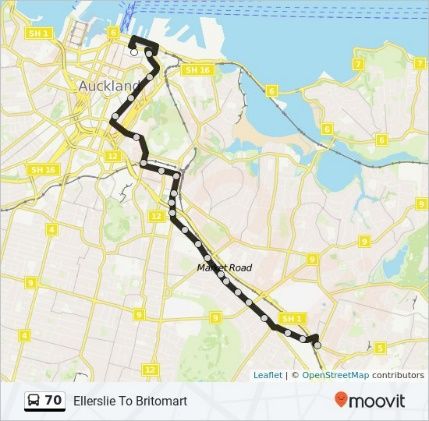
Sustainability 2020, 12, 10327                                                                                9 of 26

amount of delay-tolerant background data over the road infrastructure between two remote data
centers using bus stops in between.

1.    Data offloading for stopping stops: Recall that the objective is to use public transport vehicles to
      carry large amounts of delay-tolerant data while reducing traffic load from existing infrastructure.
      All buses pass by bus stops, and data can be offloaded as per the dwell time, enter time, exit time,
      and contact duration of the bus into the range of the deployed RSU.

                                                   tcd = ten + tdt + tex                                         (7)

where ten , tdt , tex , and tcd are the bus entering time, dwell time, exit time, and contact duration
at each bus stop, respectively. We assume that bus entering/exit speed is the same and gradually
decreases/increases with speed (s) until it further reaches the next bus stop. We state the communication
range (CR) for each bus while coming in contact with the RSU deployed at each bus stop as
Sustainability 2020, 12, x FOR PEER REVIEW                                                                  10 of 25
                                                   dex = st2 + v0 t + d                                          (8)
Where          is the maximum throughput at stay time               for all the stopping bus stops. Parent bus
where d is the distance between the RSU deployed and the bus during stay time. dex is the distance
stops
 after twill also be
         seconds    ofconsidered   underthe
                       the bus leaving     stopping
                                             stop or bus
                                                     fromstops. i is the
                                                           the range   ofrange  fromRSU.
                                                                          deployed   1 up to
                                                                                          BusNstops
                                                                                               number   of stops
                                                                                                    at stopping
 stop, ≤
(1≤              ) referring
        in this case,        to allastops
                       bus leaves         including
                                     station                 situation and therefore v0 = 0.
                                                     parent stops.
                                             from standstill

                                    Figure 4.
                                    Figure    Dataallocation
                                           4. Data allocationmodel
                                                             modelonto
                                                                   ontobuses.
                                                                       buses.

      To calculate
3.4. Data offloading data throughput,
                     for Passing Stops it is important to know the received signal power (rsp). This
depends upon the distance from the deployed RSU and the bus arrival or staying time. We will be
     The busrsp(d)
calculating    just passes
                     using through   the passing
                            the distance  between  stop
                                                      RSUwith
                                                           anda constant
                                                                log-normal  speed (i.e., s = 0),
                                                                               shadowing         andloss
                                                                                              path    there are no
                                                                                                         model   as
passengers
follows      to board  at a bus stop. In this case,  the bus comes    in  contact with  any   bus stop  for a very
short duration. Where time (t) is defined
                                      rsp(d) =asPr − 10ϕ log(dex /dre f ) + σ                                   (9)
                                                           t = 2tps                                              (17)
where Pr is the received power from RSU at reference distance dre f , ϕ is the path loss component (PLE),
σ is thet pnormally
where      s = d ex /v ps ,distributed
                            v ps is the velocity  the time Pofr can
                                         randomatvariable.          be further
                                                                passing  stops. obtained by following
                                                                                Substituting values in (5), it is:
                                                      ex = v ps ∗ t + d
                                             Pr = Ptrd−  20log 4 ∗ π ∗ dre f /λ                               (18)
                                                                                                                (10)
    Furthermore, to obtain received signal power again for passing stops is defined as
where Ptr is the transmitted power and λ is the signal wavelength in meters and can be obtained from
λ = c/f, where c is the speed of lightrsp(t)
                                       and f=isPrthe
                                                  − 10φ log(vps ∗dt +isd)the
                                                     frequency.            + σdistance from the RSU, and the(19)
                                                                                                              bus
and effective distance  can be 2d, the diameter
    The offloading efficiency of passing stop is  of the radius  coverage      area of RSU deployed  at bus stops.
Every bus will be in coverage as it starts entering at bus stops. Their data will start offloading at a

                                                      = 2                  ∗Δ                                 (20)

where j is the list of stops, where bus passes by (1 ≤ j ≤ Nps).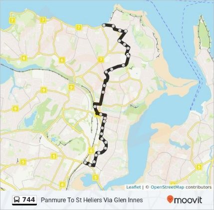
Sustainability 2020, 12, 10327 10 of 26
distance from 0 to 2d meters. Moving further, received signal power rsp also depend upon the time (t),
therefore considering dre f = 1 m, rsp with respect for time is defined.
1
rsp(t) = Pr − 10ϕ log st2 + d + σ (11)
2
We use the IEEE802.11 module as an interface to make a connection between the bus and RSU.
The maximum throughput is calculated based upon signal-to-noise ratio SNR(db), which can be
calculated as follows:
SNR(in db) = rsp(t) − nb (12)
where nb is the background noise. Furthermore, SNR(db) based upon a time can be obtained as:
1
SNR(t) = Pr − nb − 10ϕ log st2 + d + σ (13)
2
The maximum bit rates λmax rates are attained from MCS mapping tables bandwidth bw based
upon different frequencies (f ), number of spatial streams (SS), and duration of the guard interval (GI).
∀snri ≤ snr(t) < snri+1 → λmax (14)
where i = 0, 1, 2, . . . , 9 from MCS index to attain maximum bit rate and F is the mapping function.
The throughput µ(en/ex) can be obtained from the maximum data rate (λmax ) and MAC efficiency (ρ).
µen/ex = λmaxρ (15)
Hence, offloading capacity (Oc ) is the sum of the capacity for stopping bus stop, or non-stopping
bus stops as defined above as two different cases.
timax
Nstp
X X
Ostopping = µi ∗ ti + 2 µien/ex ∗ ∆ti
(16)
st st
i=1 t=0
where µist is the maximum throughput at stay time tist for all the stopping bus stops. Parent bus stops
will also be considered under stopping bus stops. i is the range from 1 up to N number of stops
(1 ≤ i ≤ Nstp ) referring to all stops including parent stops.
3.4. Data offloading for Passing Stops
The bus just passes through the passing stop with a constant speed (i.e., s = 0), and there are no
passengers to board at a bus stop. In this case, the bus comes in contact with any bus stop for a very
short duration. Where time (t) is defined as
t = 2tps (17)
where tp s = dex /vps , vps is the velocity at the time of passing stops. Substituting values in (5), it is:
dex = vps ∗ t + d (18)
Furthermore, to obtain received signal power again for passing stops is defined as
rsp(t) = Pr − 10ϕ log(vps ∗ t + d) + σ (19)Sustainability 2020, 12, 10327 11 of 26
The offloading efficiency of passing stop is
j
Nps tmax
X X
j
Opassing = 2 µps ∗ ∆t j (20)
j=1 t=0
where j is the list of stops, where bus passes by (1 ≤ j ≤ Nps ).
3.5. Total Data Offloading for NESUDA
We have analyzed offloading efficiency for two different types of bus stops. If the bus stops
for some time at any stopping bus stop, then we obtain offloading efficiency of stopping bus stop
Ostopping from equation 16. On the other hand, if the bus just passes through any passing stop, then
the offloading efficiency Opassing will be calculated from equation 20. The total offloading efficiency
O(Total) of the public transport network can be acquired from the equation
O = Ostopping + Opassing (21)
Sustainability 2020, 12, x FOR PEER REVIEW 11 of 25
By substituting (16) and (20) into (21), we have
j
timax
Nstp Nps tmax
X X X X
j (22)
(O(Total
)= )= µi ∗∗ ti +
st st + 22 / ∗∗∆t
µien/ex Δi ++
22 µps ∗ ∆t∗jΔ (22)
i=1 t=0 j=1 t=0
4. Evaluation Results
4. Evaluation Results
4.1. Case Study: Auckland Public Transport Network
4.1. Case Study: Auckland Public Transport Network
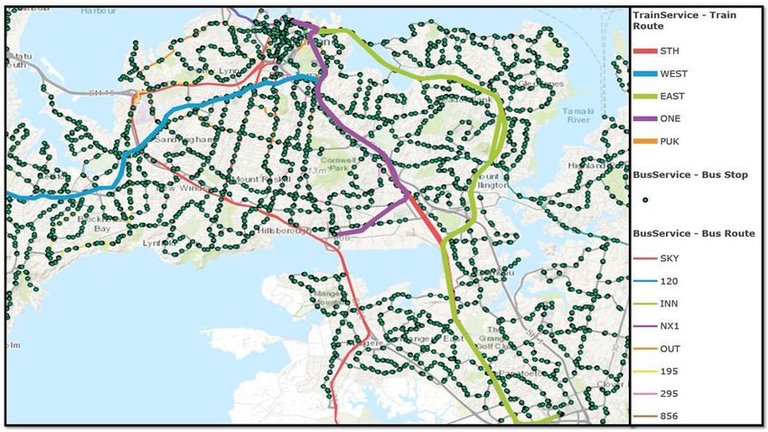
We use the Auckland city public transportation system as an example to validate our proposed
We use the Auckland city public transportation system as an example to validate our proposed
system. This data set allows us to study the spatial-temporal characteristics of the bus system to
system. This data set allows us to study the spatial-temporal characteristics of the bus system to be
be utilized for data transmission. The AT map, as shown in Figure 5, clearly shows Auckland bus
utilized for data transmission. The AT map, as shown in Figure 5, clearly shows Auckland bus routes
routes with their respective bus stops. We collected Auckland transport data sets from “Auckland
with their respective bus stops. We collected Auckland transport data sets from “Auckland Transport
Transport Open GIS data” resources. This is freely downloadable in general transit feed specification
Open GIS data” resources. This is freely downloadable in general transit feed specification (GTFS)
(GTFS) format.
format.
Figure 5.
Figure Auckland public
5. Auckland public transport
transport network.
network.
4.1.1. Data Preprocessing of Collected Dataset
The obtained dataset includes all the information related to buses and bus stops. It comprises the
trip id of a bus, timestamp, longitude, and latitude of all the bus stops, etc. These data include tripsSustainability 2020, 12, 10327 12 of 26
4.1.1. Data Preprocessing of Collected Dataset
The obtained dataset includes all the information related to buses and bus stops. It comprises the
trip id of a bus, timestamp, longitude, and latitude of all the bus stops, etc. These data include trips
over different routes with different directions, either upstream or downstream. The trips, stop_times,
and routes dataset are the baseline dataset for the analysis to get details like scheduled arrival time
and the departure time of all buses, fixed latitude and longitude positions of bus stops, which in turn
helps to compute different data features for bus arrival time prediction.
1. Calculating the distance between two bus stops
To evaluate bus arrival time, it is important to know the travel time and distance between two
consecutive bus stops. There are many techniques available for calculating the distance between two
bus stops. As defined in the description of the data set, the bus stop file contains its stop id along with
longitude and latitude attributes. We use the well-known distance computation Haversine formula [43]
to calculate distance as below:
√
D = 2r arscin( Havrsine(φ2 − φ1 + cos φ1 cos φ2 Haversine(λ2 − λ1 )) (23)
where D is the distance to be calculated, r is the radius of the earth, which is 6378.1 km, and ϕ1 , ϕ2
implies the latitude of stop1 and stop 2. λ1 and λ2 denotes the longitude of stops 1 and 2.
2. Calculating bus travel time between two bus service stops
The bus travel time is another feature to be calculated to help us with our bus arrival time
prediction. An array of timestamp values is obtained from all the bus stops spots. Eventually, this
feature from the stop time file will help to compute the travel time between consecutive bus stops and
the cumulative time taken at each bus stop. Time value in this array is in the format of “HH:MM: SS”,
so this array will be converted into seconds by the given formula.
Time (s) = HH × 3600 + MM × 60 + SS. (24)
The array will be revised with these calculated times in seconds for each consecutive bus stop.
To calculate the bus travel time for the current bus stop, the current time is subtracted from the next
time. In some cases, the bus starting from the main bus stop (source) starts with some delay. This may
be because of passengers boarding and delay in completing the existing trip. It was also seen that some
buses start 1∼2 min ahead of the scheduled time from the source.
3. Calculating speed between two bus service stops
Speed is another feature to extract to know the whole day journey of a route. It is being calculated
as distance covered per unit of time. However, we will be concerned about the average speed over the
linkages between all the bus stops of a bus route. With the extraction of this feature, we could calculate
the delay in seconds that the bus is arriving early or late on a bus route. The negative value of delay
implies that the bus is arriving late at a bus stop instead of the actual time, and the early arrival of the
bus is being denoted by the positive value. The correlation matrix helps to understand the relationship
between multiple features and attributes in the dataset to train our model. The correlation score value
varies between 0 and 1, as shown in Figure 6. If there is a strong and perfect positive correlation, then
the result is represented by a correlation score value of 0.9 or 1 or otherwise less.implies that the bus is arriving late at a bus stop instead of the actual time, and the early arrival of the
bus is being denoted by the positive value. The correlation matrix helps to understand the
relationship between multiple features and attributes in the dataset to train our model. The
correlation score value varies between 0 and 1, as shown in Figure 6. If there is a strong and perfect
positive correlation,
Sustainability then the result is represented by a correlation score value of 0.9 or 1 or otherwise
2020, 12, 10327 13 of 26
less.
Figure
Figure 6.
6. Correlation
Correlation matrix
matrix with
with feature
feature selection.
selection.
4.
4. Testingand
Testing andvalidation
validation
To test and validate our ANN model on the AT network, we used 3 months of data from 20
AprilToto test and validate
20 June. our ANN
The collected data model on the ATto
were converted network,
1410 routewe segments
used 3 months of data from
with 1048574 trips20
in April
their
to 20 June. The collected data were converted to 1410 route segments with
operational times for each bus running along the route upstream and downstream. The total bus stops1048574 trips in their
were 18,423 to be considered for RSU deployment. The AT training sample date is shown belowbus
operational times for each bus running along the route upstream and downstream. The total in
Sustainability
stops were2020, 12, to
18,423 x FOR PEER REVIEW
be considered for RSU deployment. The AT training sample date is shown13below of 25
in Figure 7. This is the ready data set used for testing and validation after applying preprocessing
Figure 7. This
functions, is the unwanted
removing ready datadata
set and
usednullforvalues.
testing Itand validation
is known afterstatic
as GTFS applying preprocessing
and includes all the
functions, removing unwanted data and null values. It is known as GTFS static
bus schedules and associated geographic information. This dataset is static and does not consider and includes all the
bus schedules and associated geographic information. This dataset is static
dwell time, passenger boarding, alighting, and other parameters. We used the first 70% as trainingand does not consider
dwell
data totime, passenger
construct boarding,
the model, alighting,
and the next 30% and otherfor
is used parameters.
testing andWe used the We
validation. firstused
70%aas training
maximum
data
of 500toiterations
construct for the our
model, and Of
model. thethe
next 30% isset,
testing used foroftesting
20% andset
the data validation.
was taken We asused a maximum
a validation test.
of
This division has been used by many researchers [44] and helps to have better prediction results test.
500 iterations for our model. Of the testing set, 20% of the data set was taken as a validation and
This division
minimum mean hasabsolute
been used by many error
percentage researchers
(MAPE). [44] and helps to have better prediction results and
minimum mean absolute percentage error (MAPE).
Figure 7. Auckland transport sample data for testing and validation.
Figure 7. Auckland transport sample data for testing and validation.
4.1.2. Auckland Transport Capacity Analysis
Our main aim was to effectively utilize the existing public transport for data dissemination. For
this evaluation, we count all the possible routes of road network from sources to destinations. This
study shows the benefits of using buses to carry data. To begin with, we first studied the potential
transmission capacity of the Auckland region for one day during weekdays. We are considering allSustainability 2020, 12, 10327 14 of 26
4.1.2. Auckland Transport Capacity Analysis
Our main aim was to effectively utilize the existing public transport for data dissemination.
For this evaluation, we count all the possible routes of road network from sources to destinations.
This study shows the benefits of using buses to carry data. To begin with, we first studied the potential
transmission capacity of the Auckland region for one day during weekdays. We are considering all
the bus services, which start at 4.30 a.m., including frequent services, local services, busway services,
and connector services. Moreover, we have inbound and outbound services for a route, but with
different bus stops. The frequency is an important factor impacting the data capacity for that time of
day. We can see the increasing trend between 7 and 9 a.m. and 4–6 p.m. These are the peak times for
the bus services with additional bus services scheduled during weekday days. We have calculated
the bus services running during daytime hours, and we assume that each bus has a capacity to carry
100 GB, and based upon this, we calculated the capacity of all Auckland regions of different areas.
We define the capacity c(i,j) as the maximum amount of data that can be transported from i to j by
buses in a time frame as follows (in Mbit/s).
X
c(i, j) = Bsi Vt (25)
t∈i,j
where Si is the storage capacity (in MBits) of every bus, B is the number of buses participating in
carrying data with storage for particular demand between locations i and j in the time T (in hours),
and Vt is the number of buses per unit of time going from i to j. The overall capacity of all buses
per day for north Auckland is 106,031.8 TB, which is massive and can be utilized efficiently to carry
data. For example, video surveillance data get captured by cameras, and the Auckland bus service
can collect data from different regions to efficiently carry that data to the transport center for further
analysis. As these data are not urgent and can be delayed up to a few hours. As said before, Auckland
central is the hub of the Auckland region. The bus services start from Auckland CBD and go in all
directions. In this way, the Auckland central area has more capacity to disseminate data as it has more
capacity for the whole day. The average capacity of Auckland central per day is 210,226.8 TB.
In South and West Auckland, there are in total 107 and 138 bus services, which run all over the
day. There is a train service in the south, which starts from Auckland central and covers central to the
south covering many suburbs. Therefore, the overall capacity of all buses per day in south Auckland
is 12,037.2 TB. As shown in Figure 8, among all of the four regions of Auckland, the North and
Central Auckland bus service haves more capacity in comparison with South and West Auckland to
disseminate data all over Auckland just because of the scheduled train services in that area. The mean
capacity of all Auckland transport bus service is 85,274.025 TB in total, which demonstrates the great
potential of using our proposed for data dissemination. These bus systems can participate in data
dissemination from one place to another which can help to leverage the heavy data burdens on the
traditional telecommunication infrastructure as well as best utilize the public transport for added value
services in the big data era.disseminate data all over Auckland just because of the scheduled train services in that area. The mean
capacity of all Auckland transport bus service is 85,274.025 TB in total, which demonstrates the great
potential of using our proposed for data dissemination. These bus systems can participate in data
dissemination from one place to another which can help to leverage the heavy data burdens on the
Sustainability telecommunication
traditional 2020, 12, 10327 15 of 26
infrastructure as well as best utilize the public transport for added
value services in the big data era.
Figure 8. Auckland public transport capacity.
Figure 8. Auckland public transport capacity.
4.2. Auckland Transport Test Trips
4.2. Auckland Transport Test Trips
To evaluate our bus arrival time prediction model, three test trips were conducted for different
To evaluate
routes of our bus public
the Auckland arrival transport
time prediction model,
network. Tablethree
2 is test trips were
presented conducted for
to demonstrate thedifferent
set of test
routes of the
trips with Auckland
random buspublic transport
trips that network.
were created byTable 2 is presented
the algorithm to demonstrate
for bus theand
route 744, 141, set of
70 test
runstrips
in the
with random bus trips that were created by the algorithm for bus route 744, 141,
afternoon hours of the day. The ANN model was trained and tested with such random observations, and 70 runs in the
afternoon hours of
and then MAPE andtheSMAPE
day. The ANN model
metrics was trained
were estimated forand tested
actual withtime
arrival suchand
random observations,
predicted bus arrival
and
timethen MAPE
values andthe
from SMAPE
ANNmetrics
model.were estimated
Figures 12–14for actual arrival
illustrate time and
the selected buspredicted
route withbusbus
arrival
stops
time values from the ANN model. Figures 9–11 illustrate the selected bus route with
(snapshot from the moovit app). This ready data set is used to train the model to predict arrival time at bus stops
(snapshot fromin
each bus stop the moovit
offline app). This ready data set is used to train the model to predict arrival time
mode.
at each bus stop in offline mode.
• Test Trip 744: The testbed selected as a sample is the Auckland Transport bus route 744. Which is
one of Auckland’s central services and connects St Heliers To Panmure via Glen Innes, considering
downstream direction covering 29 stops with trip duration for 25 min and length of route of 7 km
in between Stop 1 and Stop 29. Figure 9a illustrates the behaviors of actual and predicted bus
arrival times at each bus stop after validation of the neural network algorithm. On the x-axis,
the bus stop numbers are plotted, starting from the target station of each testing sample up to
the last destination of the bus trip. On the y-axis, the arrival time (seconds) taken at which a
bus reaches any bus stops on its route is plotted. The trained algorithm trend proves that there
is a slight difference at a few bus stops between actual and predicted arrival times. Figure 9b
represents the delay (seconds) to reach each bus stop. The negative value represents that the bus is
arriving late at each bus stop. On the other site, positive values indicate the early arrival of buses
at each stop, which ultimately represents the variation in bus arrival time. We are considering
buses to carry data with delay-tolerant features. Therefore, this much delay variation is acceptable
to use buses as another communication mode.
• Test Trip 141: The next test trip selected is number 141, which is called Henderson West Loop
Anticlockwise. This trip has 32 stops and covers the whole journey in approximately 33 min.
The bus departs from Stop A Henderson Interchange and finishes at Stop B Henderson Interchange.
The operating hours for this bus are from 05:15 to 23:15 every day, including weekend hours from
06:38 to 23:08. Same way as the previous trip, Figure 10a illustrates that there is variation between
predicted and actual arrival time. However, Figure 10b clearly shows that the bus is arriving earlyat which a bus reaches any bus stops on its route is plotted. The trained algorithm trend proves
that there is a slight difference at a few bus stops between actual and predicted arrival times.
Figure 12b represents the delay (seconds) to reach each bus stop. The negative value represents
that the bus is arriving late at each bus stop. On the other site, positive values indicate the early
Sustainability 2020, 12, 10327 16 of 26
arrival of buses at each stop, which ultimately represents the variation in bus arrival time. We are
considering buses to carry data with delay-tolerant features. Therefore, this much delay variation
is acceptable
most of the time to use buses
at each stopas except
another5 communication mode.clearly states that we can use public
or 6 bus stops, which
Test Tripas
transport 141: The next
another test trip selected
communication modeiswith
number 141, whichfeatures.
delay-tolerant is called Henderson West Loop
• Anticlockwise.
Test Trip 70: This This
testtrip
triphas70 32 stops
starts and56
from covers the whole
Customs St eastjourney in approximately
near Britomart and ends33 inmin.
StopTheA
bus departs
Botany town from
center.Stop
This A trip
Henderson
covers aInterchange and finishes
total of 46 stops at Stop B Henderson
in approximately 58 min. This Interchange.
bus route
isThe operatingevery
operational hoursday,for and
this the
busfirst
are journey
from 05:15 to 23:15
starts at 00:05every
andday,
endsincluding weekend
at 23:50 every hours
weekday,
from
and on06:38 to 23:08. Same
the weekend, it beginswayatas the am
06:15 previous trip,atFigure
and ends 23:35. 13a illustrates
Similarly, that11a
Figure there is variation
illustrates the
between
trend predicted
of actual and actual
and predicted arrival
bus arrivaltime.
timeHowever,
at each bus Figure
stop. 13b
Thisclearly showsthat
route shows thatactual
the bus
andis
arriving early
predicted arrivalmost
timeofis the time at
different oneach
eachstop except
bus stop and5 or 6 bus
never onstops, which clearly
the scheduled time. Instates that11b,
Figure we
can use public represents
delay(seconds) transport as allanother communication
the negative values and modeimplies with
thatdelay-tolerant
the bus is late features.
at each bus stop.
Test Trip 70: This test trip 70 starts from 56 Customs St east near Britomart and ends in Stop A
Botany town center. This trip covers a total of 46 stops in approximately 58 min. This bus route
Table 2. Set of test trips with the number of bus stops.
is operational every day, and the first journey starts at 00:05 and ends at 23:50 every weekday, and
on the weekend, it begins at Trip
Test 06:15 am and ends at Number
23:35. Similarly, Figure 14a illustrates the trend
of Bus Stops
of actual and predicted Testbus
trip arrival
744 time at each bus stop. 29 This route shows that actual and
predicted arrival time is different on each bus stop and never on the scheduled time. In Figure
Test trip 141 32
14b, delay(seconds) represents all the negative values and implies that the bus is late at each bus
Test trip 70 46
stop.
(a) (b)
Figure 9. Test trip 744. (a) Actual vs. Predicted arrival time. (b) Delay at each bus stop.
Figure 12. Test trip 744. (a) Actual vs. Predicted arrival time. (b) Delay at each bus stop.Sustainability 2020, 12, x FOR PEER REVIEW 17 of 25
Sustainability 2020, 12, 10327 17 of 26
Sustainability 2020, 12, x FOR PEER REVIEW 17 of 25
(a) (b)
(a) (b)
Figure 13. Test trip 141. (a) Actual vs. Predicted arrival time. (b) Delay at each bus stop.
Figure 10. Test trip 141. (a) Actual vs. Predicted arrival time. (b) Delay at each bus stop.
Figure 13. Test trip 141. (a) Actual vs. Predicted arrival time. (b) Delay at each bus stop.
(a) (b)
Sustainability 2020, 12, x FOR(a)
PEER REVIEW (b) 15 of 25
Figure 11. Test trip 70. (a) Actual vs. Predicted arrival time. (b) Delay at each bus stop.
Figure 14. Test trip 70. (a) Actual vs. Predicted arrival time. (b) Delay at each bus stop.
Figure 14. Test trip 70. (a) Actual vs. Predicted arrival time. (b) Delay at each bus stop.
Table 3 presents containing typical MAPE interpretation to analyze our ANN model results.
Table 3 presents containing typical MAPE interpretation to analyze our ANN model results.
Table 3. Mean absolute percentage error (MAPE) value and its interpretations.
Table 3. Mean absolute
MAPEpercentageInterpretation
error (MAPE) value and its interpretations.
50 Inaccurate forecasting
Table 4 is created to show the MAPE and SMAPE values calculated for each test trip, and the
Figure
Figure12. Testtrip
9. Test trip744.
744.
lowest MAPE
Table 4 isand SMAPE
created that were
to show estimated
the MAPE and for the model
SMAPE valueswas observedfor
calculated foreach
test case trip 744
test trip, andwith
the
13.91% and 0.1477 error, respectively.
lowest MAPE and SMAPE that were estimated for the model was observed for test case trip 744 with
13.91% and 0.1477 error, respectively.Sustainability 2020, 12, 10327 Figure 9. Test trip 744. 18 of 26
Figure 9. Test trip 744.
Figure 10. Test trip 141.
Figure 13. trip 141.
10. Test trip 141.
Figure 11. Test
Figure 14. trip 70.
Test trip 70.
Figure 11. Test trip 70.
Table 3 presents containing
Table 2.typical MAPE
Set of test tripsinterpretation toofanalyze
with the number our ANN model results.
bus stops.
Table 2. Set of test trips with the number of bus stops.
Test
Table 3. Mean absoluteTest Trip Number
percentage of Bus Stopsand its interpretations.
error (MAPE)
Trip Number of Busvalue
Stops
Test trip 744 29
Test trip
MAPE Test trip 141 744 29 Interpretation
32
Test trip 141 32
50 duration for 25 min and length of
considering downstream direction covering 29 stops Inaccurate
with trip duration for 25 min and length of
route of 7 km in between Stop 1 and Stop 29. Figure 12a illustrates the behaviors of actual and
route of 7 km in between Stop 1 and Stop 29. Figure 12a illustrates the behaviors of actual and
predicted bus arrival times at each bus stop after validation of the neural network algorithm. On
predicted
Table 4 is bus arrival
created times the
to show at each
MAPEbus and
stopSMAPE
after validation of the neural
values calculated fornetwork
each testalgorithm.
trip, and On
the
the x-axis, the bus stop numbers are plotted, starting from the target station of each testing
theMAPE
lowest x-axis,and
theSMAPE
bus stop numbers
that are plotted,
were estimated starting
for the model from the targetforstation
was observed of trip
test case each744testing
with
sample up to the last destination of the bus trip. On the y-axis, the arrival time (seconds) taken
sample
13.91% up to the
and 0.1477 last
error, destination of the bus trip. On the y-axis, the arrival time (seconds) taken
respectively.
Table 4. Calculated MAPE and symmetric mean absolute error (SMAPE) error values.
Test Trip MAPE SMAPE
Test Trip 744 14.98 0.1447
Test Trip 141 13.34 0.1551
Test Trip 70 19.83 0.0687You can also read