A high performance active noise control system for magnetic fields
←
→
Page content transcription
If your browser does not render page correctly, please read the page content below
A high performance active noise control system for magnetic fields
                                                    Tadas Pyragius1, a) and Kasper Jensen1, b)
                                                    1
                                                     School of Physics & Astronomy, University of Nottingham, University Park, Nottingham NG7 2RD,
                                                    United Kingdom
                                                    We present a system for active noise control (ANC) of environmental magnetic fields based on a Filtered-x
                                                    Least Mean Squares (FxLMS) algorithm. The system consists of a sensor that detects the ambient field
                                                    noise and an error sensor that measures the signal of interest contaminated with the noise. These signals are
                                                    fed to an adaptive algorithm that constructs a physical anti-noise signal cancelling the local magnetic field
                                                    noise. The proposed system achieves a maximum of 35 dB root-mean-square (RMS) noise suppression in the
                                                    DC-1 kHz band and 50 dB and 40 dB amplitude suppression of 50 Hz and 150 Hz AC line noise respectively
                                                    for all three axial directions of the magnetic vector field.

                                             Magnetically low noise environments are important          (a)
arXiv:2107.03164v1 [eess.SY] 7 Jul 2021

                                          across many metrologically relevant areas ranging from
                                          medical imaging of biomagnetic fields from the heart
                                          and brain to non-destructive evaluation of car batteries
                                          and scanning electron microscopy to name just a few1–3 .
                                          Currently, optically pumped magnetometers (OPMs) are
                                          state of the art magnetic field sensors and are a promising
                                          alternative to conventional SQUID and fluxgate magne-
                                          tometers in both shielded and unshielded conditions4,5 .
                                                                                                        (b)
                                          A wider adoption of quantum magnetometers for ultra-
                                          low field precision measurements has been limited to
                                          magnetically shielded environments due to large exter-
                                          nal magnetic field noise, making such setups expensive.
                                          Conventionally, partial magnetic field noise cancellation
                                          is achieved via a combination of proportional-integral-
                                          derivative (PID) controllers which are sometimes com-
                                          bined with a feed-forward system6–10 . Whilst these sys-
                                          tems are effective in field noise compensation and control
                                          they require extensive hands on tuning which is heavily
                                                                                                        FIG. 1. (a) Basic implementation of active noise control in the
                                          dependent on the implemented hardware constraints. As         acoustic domain. Here a noise reference microphone listens to
                                          a result, the tuning parameters cannot be easily trans-       unwanted environmental noise and feeds that information to
                                          ferred from one system to another. Furthermore, the           the adaptive algorithm. The adaptive algorithm then cal-
                                          performance of the noise suppression can be additionally      culates the anti-noise signal and outputs it through a noise
                                          limited by hardware and processing delays and system          cancelling speaker. The error microphone measures the noise
                                          imperfections which often cannot be compensated for.          + anti-noise signal and feeds it back to the adaptive algorithm
                                          In cases where the focus is on unwanted periodic envi-        for adjustment if necessary. (b) Analogous implementation of
                                          ronmental noise signals e.g. 50 Hz AC line noise and          active noise control in the magnetic field domain. Here the
                                          its corresponding harmonics, adaptive approaches have         microphones are replace by field sensitive magnetometers and
                                                                                                        the compensation is achieved by magnetic field coils.
                                          been implemented11,12 . However, as before, some of these
                                          methods require extensive manual tuning of the filter co-
                                          efficients as well as limiting the compensation to fixed AC
                                          noise frequency signals. Finally, it is often the case that   Active noise control (ANC) is achieved by introducing a
                                          the noise environment as well as the transfer function of     canceling “anti-noise” signal through a secondary source.
                                          the system are not known in advance or cannot be ade-         The secondary source is driven by an electronic system
                                          quately modelled rendering these methodologies unable         which utilises a specific signal processing algorithm
                                          to cope.                                                      (such as an adaptive algorithm) for the particular
                                                                                                        cancellation scheme, see Fig. 1. This technique is widely
                                             In this work, we demonstrate how these technical           exploited in noise cancelling headphone technology,
                                          issues can be overcome using an active magnetic field         vibration control, as well as exhaust ducts in ventilation
                                          compensation method based on adaptive filtering.              and cooling systems13–16 . Whilst adaptive filtering
                                                                                                        techniques have been demonstrated in unwanted noise
                                                                                                        cancellation of electric and magnetic fields in the context
                                                                                                        of electrocardiography (ECG) and magnetocardiography
                                          a) Electronic   mail: t.pyragius@gmail.com                    (MCG), the noise cancellation was performed on the
                                          b) Electronic   mail: kasper.jensen@nottingham.ac.uk          acquired data17,18 . This process is known as adaptive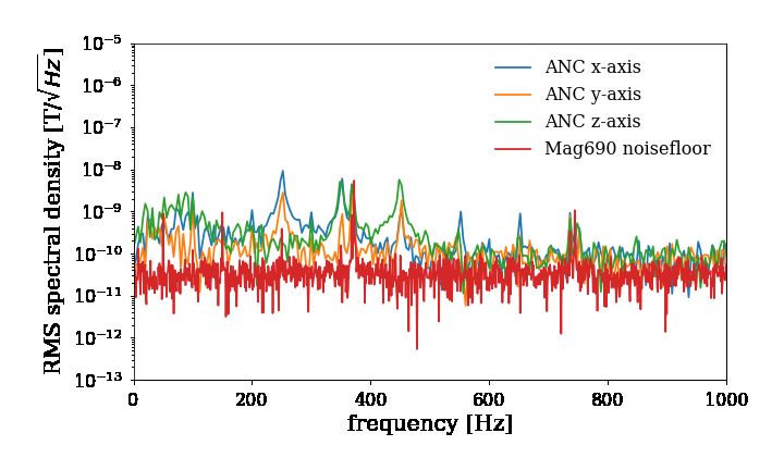
2

noise cancellation19 . In contrast, active noise control      (a)
(ANC), generates a physical anti-noise signal11,16 . This
results in a number of advantages over adaptive noise
cancellation techniques. First, the the noise signals in
the environment are typically orders of magnitude larger
than the signals of interest (e.g. magnetocardiography
signals in pT range compared to the 50 Hz line noise
in nT). This results in the requirement for a larger
dynamic range which reduces the signal resolution of
the signals of interest due to the limited number of bits
in the analog-to-digital conversion (ADC). The ANC            (b)
system cancels the physical noise signals which enables
one to reduce the analog input range for the same
number of bits, thus increasing the signal resolution and
reducing the noise floor. In the context of OPMs, and in
particular, spin-exchange relaxation-free (SERF) OPMs
one of the key feature that determines the sensitivity
of an OPM is its intrinsic linewidth20 . When the
environmental noise (e.g. 50 Hz noise) is larger than the
OPM linewidth, this broadens the linewidth and reduces
the sensitivity. ANC reduces the ambient magnetic
field noise which in turn reduces the OPM linewidth
increasing its sensitivity thus enabling its operation in     FIG. 2. (a) Theoretical structure of the secondary path H(z).
otherwise environmentally noisy conditions.                   (b) Experimental structure of the secondary path in the con-
                                                              text of magnetic field generation and measurement. Here the
   This paper is organised as follows; Section I briefly      white noise signal is fed to the digital-to-analog converter
introduces the formalism of signal discretization in the      (DAC) driving a bipolar current source (BCS) with uniform
context of digital signal processing which is used through-   field coils. The same white noise signal is fed to the adaptive
out this work to compute the secondary path effects and       algorithm as a reference. An error reference magnetometer
calculate the corresponding anti-noise signal using adap-     measures the generated white noise field which is then used
tive algorithms. Section II and III walks through the         to calculate the error signal and adjust the secondary path co-
motivation and process of secondary path modelling and        efficients. Here the secondary path H(z) consists of a DAC,
                                                              BCS, coils, magnetometer and an ADC with an anti-aliasing
its application to anti-noise generation via the filtered-
                                                              filter (not shown).
x Least Mean Squares (FxLMS) algorithm. Section IV
contains the results and discussion of the active noise
control system for magnetic field noise cancellation, its
scope, limitations and potential improvements. The last       This kernel transformation enables easy signal manipu-
section sets out the conclusion.                              lation using operations such as convolution. In discrete
                                                              system control a signal input with a system’s transfer
                                                              function producing an output is a convolution of the in-
I. THE Z-TRANSFORM FOR DISCRETE TIME
SIGNALS                                                       put signal x(n) and the system transfer function t(n)
                                                              which in a discrete z-transform is nothing but a product
                                                              of the two functions, i.e.
  A discrete time signal can be represented by a weighted
sum of delayed impulses such that
                                                                                    ∞
                  ∞                                                                 X
                                                                     (x ∗ y)[n] =         x(k)t(n − k) → X(z)T (z).      (4)
                  X
                                               +
         x(n) =         x(k)δ(n − k), ∀ n, k ∈ Z .     (1)
                                                                                    k=0
                  k=0

To express the above more conveniently and remove the
impulse response part, we can introduce a transform ker-      Due to the complexity of adaptive filters they cannot be
nel which maps the impulse response with a delay to           trivially implemented on analog electronic platforms. As
                                                              a result, adaptive filter technology is usually deployed on
                        δ(n − k) → z −k                (2)    digital platforms such as application specific integrated
which allows us to transform the discrete time signal x(n)    circuits (ASICs) acting as digital signal processing (DSP)
in terms of variable z                                        chips or field-programmable gate arrays (FPGAs). These
                     X∞                                       digital platforms deal with discrete signals and thus re-
             X(z) =      x(k)z −k , ∀ k ∈ Z+ .         (3)    quire the mathematical formalism of discrete time sig-
                        k=0                                   nals.
3
(a)
(b)
FIG. 3. (a) Theoretical structure of the primary and secondary paths. The ANC box contains the algorithmic elements of the
adaptive filter that generates an anti-noise signal. Here we assume that the primary path P (z) transfer function does not have
an appreciable effect on the signal detected at the sensor. (b) Experimental structure of the primary and secondary paths in
the context of magnetic field generation and measurement. The ANC algorithm is contained within the FPGA chip.
II. SECONDARY PATH MODELLING where E is the expectation value, Var is the variance
with a value σ 2 and the last term is the auto-correlation
between the two time delayed white noise signals. The
For a broadband ANC system, the first stage of im-
white noise signal is fed to a bipolar current source which
plementation consists of modelling the secondary path,
drives a pair of Helmholtz coils. Simultaneously, we use
see Fig. 2 (a). The secondary path takes into account
the generated y(n) white noise as a reference for the
of the hardware effects of the output for a given input
secondary path estimate filter C(z) and the least-mean-
signal. The generated signal is detected by a sensor with
squares (LMS) adaptive algorithm. The generated white
a transfer function which modifies the measured signal.
noise magnetic field is sensed by a fluxgate magnetometer
This signal is then propagated through the system which
(Bartington Mag690) and after an anti-aliasing filter is
further modifies the signal. We want to compensate for
fed into an analog-to-digital converter. The sensed mag-
these secondary path effects. This requires one to esti-
netic field corresponds to our secondary path response
mate the approximate secondary path response i.e. we
e(n). For the adaptive model, the computed response
want to find filter coefficient transfer function which can
r(n) is given by
effectively approximate the transfer function of the sec-
ondary path, i.e., C(z) ≈ H(z), which corresponds to M
X −1
discrete transfer functions of the estimated and actual r(n) = ci (n)y(n − i), (8)
secondary paths respectively. To do this, we generate a i=0
white noise signal, y(n) which satisfies
where n is the discrete time increment index, ci (n) is the
ith filter coefficient of the discrete transfer function of the
E[y(n)] = 0, (5) estimated secondary path C(z) (equivalent to an adap-
Var[y(n)] = σ ,2
(6) tive filter) and M is the total number of taps in the adap-
+
tive filter. An adaptive filter is a finite-impulse response
E[y(n) ∗ y(n − k)] = 0, ∀ k ∈ Z , (7) (FIR) filter. The number of filter taps relate to the fre-4
quency resolution of the filter by fres = fs /M , where IV. EXPERIMENTAL IMPLEMENTATION
fs is the sampling rate. The coefficients of the adaptive
FIR filter ci (n) are the quantized values of the impulse A. Outline of the ANC procedure
response of the frequency transfer function21 . The com-
puted response r(n) of the adaptive filter is then com- Applications of active noise control in noise cancelling
pared with the measured response of the system e(n) systems generally deal with AC coupled signals (e.g.
which allows us to compute the error e0 (n) acoustic or vibration signals). This becomes problem-
atic when a signal acquires a DC component which is the
e0 (n) = e(n) − r(n). (9)
case in ANC applications of magnetic field cancellation
The measured error can then be used to update the filter due to an Earth’s field component. A DC component
coefficients of the secondary path estimate C(z) affects the secondary path analysis by biasing the filter
coefficients which render the cancellation system ineffec-
ci (n + 1) = ci (n) + µsp e0 (n)y(n − i), (10) tive. As a result, in order to obtain a good estimate
for the secondary path, C(z), one must cancel the DC
where µsp is the step size of the update during secondary component of the ambient magnetic field and only then
path modelling and must satisfy11 proceed with the online secondary path estimation. This
step is achieved by a PID controller which pre-stabilises
1 the magnetic field around zero. The output voltage sent
0 < µsp < , (11)
M Py to the bipolar current source that approximately cancels
the Earth’s field is then used as a DC control during the
where Py is the power of the signal y(n). With the up- secondary path analysis combined with the white noise
dated values of the coefficients ci (n) and a new secondary reference signal for impulse response modelling with the
path estimate C(z) the procedure is repeated iteratively PID switched off. This ensures that the generated mag-
to compute the new error value and update the corre- netic field signals are centered around zero without any
sponding coefficients. After some time, the iterative pro- DC offset. The secondary path modelling is run sequen-
cedure is stopped. The final computed secondary path tially for each magnetic field vector axis individually for
coefficients c(i) and the estimated secondary path are a given duration Tsp and a step size µsp . The estimated
used in the next stage of active noise control using the secondary path coefficients are then used to construct a
FxLMS algorithm. secondary path response filter which enables the FxLMS
algorithm to calculate the anti-noise signal in active noise
control. The algorithm is deployed on NI’s sbRIO-9627
III. FILTERED LEAST MEAN SQUARES (FxLMS)
FPGA and controlled using LabVIEW with NI’s propri-
ALGORITHM
etary adaptive filter toolkit22 .
With the estimated effect of the secondary path the
next stage involves actively compensating for the noise. B. Secondary Path Estimation
A reference noise signal x(n) is propagated through the
estimated secondary path C(z) which yields the filtered
The secondary path estimation follows an experimen-
version of the reference noise signal
tal setup depicted in Fig. 2 (b). A band limited white
M
X −1 noise signal is generated within the FPGA architecture
x0 (n) = c(i)x(n − i). (12) and is used to drive a bipolar current source with a pair
i=0 of Helmholtz coils producing a uniform white noise mag-
netic field around zero. The generated magnetic field
We then proceed to compute the anti-noise signal is sensed by the error reference fluxgate magnetometer
which is then fed in to the LMS algorithm on the FPGA
M −1
X to compute the error and adjust the filter coefficients
y(n) = wi (n)x(n − i), (13)
which attempt to minimise the error. The filter coeffi-
i=0
cients allow one to construct an estimate of the impulse
where wi (n) is the ith coefficient of the adaptive filter response of the secondary path, see Fig. 4 for results.
W (z). The adaptive coefficients are then updated ac- The profile of the secondary path impulse response de-
cording to pends on a number of various physical properties of the
system such as anti-aliasing filters used for the ADCs,
wi (n + 1) = wi (n) − µanc e(n)x0 (n − i), (14) transfer functions of the coils, bipolar current source etc.,
as well as the relative gains of the input and output sig-
where e(n) is the error reference signal and µanc is the nals. In our experimental setup the 3-axis system has
ANC filter update step size, where typically µsp 6= µanc . identical hardware and software implementation includ-
The procedure is repeated. See Fig. 3 for schematic de- ing the anti-aliasing filters and the coils (near identical
tails. resistance, inductance, number of turns). Consequently,5
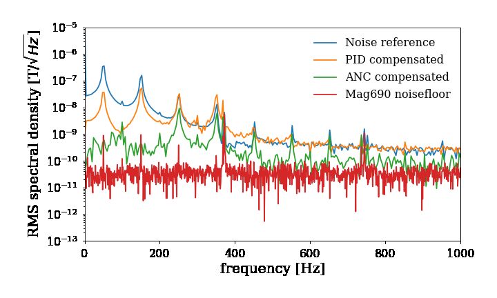
mode. Fig. 5 (a) shows the time trace comparison be-
tween the ambient field noise with and without the ANC
engaged with Figs. 5 (b-c) detailing the frequency band
performance of ANC for each vector direction. As can
be seen from the figure the ANC system is capable of
almost completely suppressing the 50 Hz and its third
harmonic, 150 Hz. This corresponds to 50 dB and 40 dB
amplitude suppression respectively with respect to the
noise reference. Moreover, we find that the ANC perfor-
mance is better than the conventional approach using a
PID controller. Fig. 5 (b) shows the ANC performance
for all 3 axial directions. One can observe from the fig-
ure that ANC is very effective in cancelling the harmonic
noise in the DC−1 kHz range with biggest noise reduc-
FIG. 4. Experimentally obtained secondary path estimates tion at lower frequencies. The noise performance is fur-
for all three axial directions. Here we have the finite impulse ther broken down over different bandwidths, see Table I.
response of a filter as a function of filter taps. The number
The 1 kHz bandwidth corresponds anti-aliasing termi-
of filter taps relate to the frequency resolution of the filter by
fres = fs /M , where fs is the sampling rate. We observe that
nated bandwidth of the analog acquisition which roughly
the impulse response is shifted because the filter only operates corresponds to the bandwidth of Mag690 fluxgate magne-
on available samples with some additional delay. For an ideal tometer. The maximum RMS noise suppression is around
low-pass filter, the filter coefficients follow a sinc function and 35 dB in the 1 kHz band. Commercial SERF OPMs have
the delay is given by (M −1)/2fs . The secondary path consists a typical bandwidth of 150 Hz and a dynamic range of
of a DAC, bipolar current source (BCS), fluxgate (Mag690), ±5 nT and require an ambient magnetic field to be be-
anti-aliasing low-pass filter (LP) and ADC. In this case the low 50 nT23 . As seen in Table I, we achieve 3 − 7 nT
specification for each hardware channel is the same giving rise RMS noise in a 150 Hz bandwidth. With just a mod-
to identical secondary path coefficients. est improvement of the performance of our ANC system,
it would therefore be possible to operate a SERF OPM
in unshielded conditions. We also note that the labora-
the estimated secondary paths using the same experimen- tory where the ANC system was deployed is exceptionally
tal parameters are to a good approximation equivalent. noisy due to high current experiments running in close
proximity. In typical lab environments, the RMS mag-
netic field noise is in < 100 nT range9,10 .
C. Active Noise Control using FxLMS algorithm
The experimental layout of the FxLMS algorithm for D. Performance limits and considerations
active noise control is shown in Fig. 3 (b). Here the
reference and error fluxgate magnetometers read the am- The performance of an FxLMS-based ANC system is
bient and compensated magnetic fields which are fed to limited by a number of factors. First, the control and
the FxLMS algorithm. The FxLMS algorithm compen- sensing hardware imposes limits on the secondary path
sates for the secondary path, adjusts the filter coefficients impulse response as well as the bandwidth. If the group
and computes an anti-noise signal y(n) (see eqns. 12-14), delays introduced by the hardware are large resulting
which drives the bipolar current source controlling a pair in a long impulse response the FxLMS algorithm will
of Helmholtz coils to produce a uniform anti-noise mag- not be able to compensate well for the noise. This
netic field. The active noise control system is initialised can be especially problematic if aggressive (high-order)
sequentially for each magnetic field vector axis. Once the anti-aliasing filters are used which introduce long group
compensation reaches a steady state limit the ANC sys- delays. To circumvent this, a low order low pass filter
tem is disabled and the compensation is initialised for the can be used. This, however, comes at the expense of
next axis until a steady state is reached there and so on. having to increase the sampling rate (oversampling).
Once each axial direction has converged with optimum This introduces further limitations due to the fact that
filter coefficients, the ANC system is then switched on there is an upper time limit of the processing speed of
simultaneously for all three axial directions. In this con- the FxLMS algorithm. Another way to counter the long
figuration the ANC algorithm is capable of compensating delay response is to increase the filter length. However,
for AC as well as DC fields without requiring additional this increases the processing time and resources on the
Earth’s field nulling. The initial DC field nulling is only FPGA hardware and reduces the maximum bandwidth.
required during the secondary path estimation. Due to Moreover, whilst increasing the filter length reduces the
cross-talk between each axis direction, some field leak- steady state error, it degrades the rate of convergence
age occurs and the FxLMS algorithm has to re-adjust process to reach the steady state error24 .
the optimum filter coefficients when operated in 3-axis6
TABLE I. RMS noise performance of PID and ANC sys-
(a)
tems benchmarked against the environmental noise. Bot-
tom table expresses the RMS magnetic field noise converted
to frequency using the gyromagnetic ratio of Cesium, γ =
350 kHz/G. Cesium is a common atomic species used in
OPMs. The frequency values on the axis row correspond to
the bandwidths for which the noise performance is calculated
for.
Noise PID ANC
Axis 1 kHz 150 Hz 1 kHz 150 Hz 1 kHz 150 Hz
x-axis 800 nT N/A 112 nT 80 nT 16 nT 7 nT
y-axis 150 nT N/A 35 nT 25 nT 7 nT 3 nT
z-axis 450 nT N/A 23 nT 16 nT 12 nT 7 nT
(b)
Noise PID ANC
Axis 1 kHz 150 Hz 1 kHz 150 Hz 1 kHz 150 Hz
x-axis 2800 Hz N/A 392 Hz 280 Hz 56 Hz 24.5 Hz
y-axis 525 Hz N/A 123 Hz 87.5 Hz 24.5 Hz 10.5 Hz
z-axis 1580 Hz N/A 80.5 Hz 56 Hz 42 Hz 24.5 Hz
netic field noise profiles of varying amplitude, spectral
profile and phase. Due to the principle of superposi-
tion and field decay, the resulting environmental noise
(c)
will have spatial and temporal inhomogeneities. More-
over, if any conductive objects are present in the vicinity
of the noise or error reference magnetometers, the time
varying magnetic fields will induce eddy currents in the
conductive objects which will produce their own respec-
tive magnetic fields25 . As a result, the relative position
of the noise and error reference magnetic field sensors can
have a significant effect on the noise cancellation of the
ANC system since it fundamentally relies on common-
mode noise cancellation. The degree of noise coherence
between the error and reference sensor can be quantified
by the coherence function
2
FIG. 5. (a) Time trace of the error magnetometer signal be- |Sx,y (f )|
γ 2 (f ) = , (15)
fore and after applying active noise control. The time trace for Sx (f )Sy (f )
the ANC OFF case has been offset to subtract the DC Earth’s
field for visualisation. (b) Root mean square amplitude spec- where Sx (f ) and Sy (f ) are power spectral densities of the
tral density of the magnetic field signals. The noise reference error and noise reference signals and Sx,y (f ) is the cross
fluxgate which monitors the ambient field environment. ANC power spectral density. The coherence function takes the
compensated is the magnetic field measured by the error mag- range
netometer which monitors the cancelled magnetic field noise.
The PID compensated noise is the error magnetometer mea- 0 ≤ γ 2 (f ) ≤ 1, (16)
suring the noise performance using conventional proportional-
integral-differential controller. (c) ANC performance RMS where a zero value of coherence implies no correlation be-
amplitude spectral density for all three axial directions run tween the signals and a value of 1 implies perfect signal
simultaneously. The Mag690 noisefloor is obtained inside a correlation. Real-time estimation of the noise coherence
4-layer µ-metal shield in an open loop configuration. between the noise reference and the error sensors can be
used to determine the optimal placement of the noise ref-
erence magnetometer relative to the error magnetometer.
Another highly crucial ingredient in determining the The theoretical maximum cancellation of the noise for a
performance of the ANC system is the noise coherence. given frequency band is given by26
In real world environments multiple magnetic field noise
α(f ) = −10 log10 1 − γ 2 (f ) [dB].
sources may be present. These will have their own mag- (17)7
Active noise control systems applied to cancel the ACKNOWLEDGEMENTS
acoustic noise can inadvertently suffer with echo effects
which occur as a result of the sound generated by the This work was supported by the UK Quantum Tech-
noise cancelling speaker propagating and reaching the nology Hub in Sensing and Timing, funded by the En-
noise reference microphone. Echo effects can also occur gineering and Physical Sciences Research Council (EP-
when attempting to cancel the magnetic field noise if SRC) (EP/T001046/1), the Nottingham Impact Accel-
the magnetic field produced by the coils is sensed by erator / EPSRC Impact Acceleration Account (IAA),
the noise reference magnetometer (which is located and by Dstl via the Defence and Security Accelerator:
at a finite distance from the coils). If such fields are www.gov.uk/dasa. We thank Yonina Eldar for reading
strong they can inadvertently introduce a feedback the manuscript.
loop in the ANC system rendering it unstable. One
solution is to place the noise reference sensor further
away from the coils. However, this comes at the DATA AVAILABILITY
expense of reducing the noise coherence between the
reference and error magnetometers25 . An alternative is
The data that support the findings of this study are
to introduce adaptive echo cancellation through primary
available from the corresponding author upon reasonable
path modelling which is then incorporated into the
request.
FxLMS algorithm27,28 . Another strategy to mitigate
field echo contamination is to use coil geometries that
have one-sided flux pattern which keeps the generated REFERENCES
anti-noise field within the inner coil structure where
the error sensor resides. This can be achieved through
Halbach-type electromagnet architecture29,30 . Finally, 1 R. Fenici, D. Brisinda, A. M. Meloni, “Clinical application of
the noise floor of the in-loop error and noise reference magnetocardiography”, Expert Rev. Mol. Diagn., 5(3):291-313
sensors will ultimately impose an upper limit on the (2005).
2 Y. Hu, G. Z. Iwata, M. Mohammadi, E. V. Silletta, A. Wick-
noise suppression of the environmental field. enbrock, J. W. Blanchard, D. Budker, and A. Jerschow, “Sensi-
tive magnetometry reveals inhomogeneities in charge storage and
The FxLMS algorithm used in this work is by far weak transient internal currents in Li-ion cells”, PNAS May 19,
the most common approach deployed in active noise 117 (20) 10667-10672 (2020) .
3 M. Pluska, A. Czerwinski, J. Ratajczak, J. Katcki, R Rak, “Elim-
control. However, there exists an extensive family
ination of scanning electron microscopy image periodic distor-
of alternative adaptive algorithms which possess a tions with digital signal-processing methods”, J. Microsc. 224(Pt
varying degree of capabilities ranging from the speed 1):89-92 (2006).
4 D. Budker and D. F. Jackson Kimball, “Optical Magnetometry”,
of convergence to the value of steady state error and
computational complexity16,31 . Depending on the con- Cambridge University Press, Cambridge, ISBN: 9781107010352
(2013).
ditions for ANC, a different adaptive algorithm could be 5 A. Grosz, M. J. Haji-Sheikh, and S. C. Mukhopadhyay, “High
employed to enable better performance e.g. greater noise Sensitivity Magnetometers”, Springer, ISBN: 9783319340708
suppression at the expense of increased hardware and (2017).
6 D. Platzek, H. Nowak, F. Giessler, J. Röther, and M. Eiselt,
processing requirements. This also applies to secondary
path modelling stage. “Active shielding to reduce low frequency disturbances in direct
current near biomagnetic measurements”, Rev. Sci. Inst. 70, 2465
(1999).
7 R. Zhang, Y. Ding, Y. Yang, Z. Zheng, J. Chen, X. Peng, T. Wu
V. CONCLUSIONS and H. Guo, “Active Magnetic-Field Stabilization with Atomic
Magnetometer”, Sensors, 20(15), 4241 (2020).
8 R. Zhang, W. Xiao, Y. Ding, Y. Feng, X. Peng, L. Shen, C.
We have shown that active noise control is an effective Sun, T. Wu, Y. Wu, Y. Yang, Z. Zheng, X. Zhang, J. Chen,
technique for broadband magnetic field noise cancella- H. Guo, “Recording brain activities in unshielded Earth’s field
with optically pumped atomic magnetometers”, Sci. Adv. 2020;
tion. It requires minimal hands on approach to tuning 6:eaba8792 (2020).
for optimal performance and is flexible for deployment 9 B. Merkel, K. Thirumalai, J. E. Tarlton, V. M. Schäfer, C. J.
across different hardware architectures. Moreover, in sit- Ballance, T. P. Harty, and D. M. Lucas, “Magnetic field stabi-
uations where the signals of interest are much smaller lization system for atomic physics experiments”, Rev. Sci. Inst.
than the ambient noise, active noise control implementa- 90, 044702 (2019).
10 K. Xiao, L. Wang, J. Guo, M. Zhu, X. Zhao, X. Sun, C. Ye,
tion can be used to increase the signal to noise ratio by in- and X. Zhou, “Quieting an environmental magnetic field without
creasing the resolution of the measurement via a reduced shielding”, Rev. Sci. Inst. 91, 085107 (2020).
input range over the same number of bits. Finally, for 11 S. M. Kuo, I. Panahi, K. M. Chung, T. Horner, M. Nadeski, J.
highly sensitive devices such as optically pumped mag- Chyan, “Design of active noise control systems with the tms320
netometers where the intrinsic device sensitivity strongly family” (1996).
12 G. Bevilacqua, V. Biancalana, Y. Dancheva, and A. Vigilante,
depends on the ambient field noise, an active noise control “Self-Adaptive Loop for External-Disturbance Reduction in a
system can be used to enable highly sensitive operation Differential Measurement Setup”, Physical Review Applied, 11,
in magnetically unshielded environments. 014029 (2019).8
13 S. M. Kuo, S. Mitra, W. Gan, “Active noise control system for 22 LabVIEW Digital Filter Design Toolkit, LabVIEW.
headphone applications”, IEEE Transactions on Control Systems 23 QZFM Gen-2 Technical Specifications, https://quspin.com/
Technology, Volume: 14, Issue: 2 (2006). products-qzfm/.
14 J. C. Driggers, M. Evans, K. Pepper, and R. Adhikari, “Active 24 I. T. Ardekani and W. Abdulla, “FxLMS-based active noise con-
noise cancellation in a suspended interferometer”, Rev. Sci. Inst. trol: A quick review”, APSIPA, ASC (2011).
83, 024501 (2012). 25 P. J. M. Wöltgens and R. H. Koch, “Magnetic background noise
15 K. Chen, C. Chang, S. M. Kuo, “Active noise control in a duct cancellation in real-world environments”, Rev. Sci. Inst. 71, 1529
to cancel broadband noise”, Materials Science and Engineering, (2000).
237 (2017). 26 S. M. Kuo and D. R. Morgan, “Active Noise Control Systems
16 S. M. Kuo, D. R. Morgan, “Active noise control: a tutorial re- Algorithms and DSP Implementations”, New York, NY: John
view”, Proceedings of the IEEE, Volume: 87, Issue: 6 (1999). Wiley & Sons, (1996).
17 V. Tiporlini, K. Alameh, “Optical Magnetometer Employing 27 M. M. Sondhi, “An adaptive echo canceller”, The Bell System
Adaptive Noise Cancellation for Unshielded Magnetocardiogra- Technical Journal, Volume: 46, Issue: 3 (1967).
phy”, Universal Journal of Biomedical Engineering 1(1): 16-21 28 M. Kazuo, U. Shigeyuki, A. Fumio, “Echo Cancellation and Ap-
(2013). plications”, IEEE Communications Magazine, 28 (1): 49–55,
18 N. V. Thakor, Y. S. Zhu, “Applications of adaptive filtering ISSN 0163-6804 (1990).
to ECG analysis: noise cancellation and arrhythmia detection”, 29 K. Halbach, “Design of permanent multipole magnets with ori-
IEEE Transactions on Biomedical Engineering, Volume: 38, Is- ented rare earth cobalt material”, Nuclear Instruments and
sue: 8 (1991). Methods. 169 (1): 1–10 (1980).
19 B. Widrow, J.R. Glover, J. M. McCool, J. Kaunitz, C. S. 30 B. Shen, L. Fu, J. Geng, X. Zhang, H. Zhang, Q. Dong, C. Li,
Williams, R. H. Hearn, J. R. Zeidler, Jr. Eugene Dong, R. C. J. Li, T. A. Coombs, “Design and Simulation of Superconduct-
Goodlin, “Adaptive noise cancelling: Principles and applica- ing Lorentz Force Electrical Impedance Tomography (LFEIT)”,
tions”, Proceedings of the IEEE, Volume: 63 Issue: 12 (1975). Physica C: Superconductivity and its Applications, Volume 524,
20 J. C. Allred, R. N. Lyman, T. W. Kornack, and M. V. Roma- Pages 5-12 (2016).
lis, “High-Sensitivity Atomic Magnetometer Unaffected by Spin- 31 R. Martinek, R. Kahankova, J. Nedoma, M. Fajkus, M. Skacel,
Exchange Relaxation”, Phys. Rev. Lett. 89, 130801 (2002). “Comparison of the LMS, NLMS, RLS, and QR-RLS algorithms
21 W. Kester, “Mixed-Signal Design Seminar”, Analog Devices, for vehicle noise suppression”, ICCMS 2018: Proceedings of the
ISBN-0-916550-08-7 (1991). 10th International Conference on Computer Modeling and Sim-
ulation (2018).You can also read