A global ozone profile climatology for satellite retrieval algorithms based on Aura MLS measurements and the MERRA-2 GMI simulation
←
→
Page content transcription
If your browser does not render page correctly, please read the page content below
Atmos. Meas. Tech., 14, 6407–6418, 2021
https://doi.org/10.5194/amt-14-6407-2021
© Author(s) 2021. This work is distributed under
the Creative Commons Attribution 4.0 License.

A global ozone profile climatology for satellite retrieval
algorithms based on Aura MLS measurements and
the MERRA-2 GMI simulation
Jerald R. Ziemke1,2 , Gordon J. Labow3 , Natalya A. Kramarova1 , Richard D. McPeters1 , Pawan K. Bhartia1 ,
Luke D. Oman1 , Stacey M. Frith3 , and David P. Haffner3
1 NASA  Goddard Space Flight Center, Greenbelt, Maryland, USA
2 Goddard Earth Sciences Technology and Research (GESTAR) and Morgan State University, Baltimore, Maryland, USA
3 SSAI, Lanham, Maryland, USA

Correspondence: Jerald R. Ziemke (jerald.r.ziemke@nasa.gov)

Received: 29 May 2021 – Discussion started: 22 June 2021
Revised: 19 August 2021 – Accepted: 31 August 2021 – Published: 5 October 2021

Abstract. A new atmospheric ozone profile climatology has        terannual variability in global stratospheric ozone including
been constructed by combining daytime ozone profiles from        quasi-biennial oscillation (QBO) signatures.
the Aura Microwave Limb Sounder (MLS) and Modern-Era
Retrospective Analysis for Research Applications version 2
(MERRA-2) Global Modeling Initiative (GMI) model simu-
                                                                 1   Introduction
lation (M2GMI). The MLS and M2GMI ozone profiles are
merged between 13 and 17 km (∼ 159 and 88 hPa), with             McPeters and Labow (2012) (hereafter, ML) and Labow et al.
MLS used for stratospheric and GMI for primarily tropo-          (2015) combined ozone profile data from ozonesondes and
spheric levels. The time record for profiles from MLS and        the Aura Microwave Limb Sounder (MLS) (Livesey et al.,
GMI is August 2004–December 2016. The derived seasonal           2011) to use as climatological a priori information for satel-
climatology consists of monthly zonal-mean ozone profiles        lite retrievals of ozone. These ozone profile climatologies
in 5◦ latitude bands from 90◦ S to 90◦ N covering altitudes      were constructed by merging ozonesondes in the troposphere
(in Z ∗ log-pressure altitude) from zero to 80 km in 1 km        with satellite ozone in the stratosphere and mesosphere. For
increments. This climatology can be used as a priori infor-      the ML climatology, the stratosphere–mesosphere portion of
mation in satellite ozone retrievals, in atmospheric radiative   the climatological ozone profiles was based on averaging
transfer studies, and as a baseline to compare with other        MLS daytime and nighttime limb measurements. The mix
measured or model-simulated ozone. The MLS/GMI sea-              of daytime and nighttime measurements led to smearing of
sonal climatology shows a number of improvements com-            the ozone diurnal cycle in the upper stratosphere and lower
pared with previous ozone profile climatologies based on         mesosphere.
MLS and ozonesonde measurements. These improvements                 The limited amount and sparse spatial coverage of
are attributed mostly to continuous daily global coverage        ozonesonde data have led us to now use the NASA God-
of GMI tropospheric ozone compared with sparse regional          dard Earth Observing System (GEOS) Global Modeling Ini-
measurements from sondes. In addition to the seasonal cli-       tiative (GMI) model as a substitute for the ozonesonde data
matology, we also derive an additive climatology to account      in the lower atmosphere. The GMI model uses Modern-Era
for interannual variability in stratospheric zonal-mean ozone    Retrospective Analysis for Research Applications version 2
profiles which is based on a rotated empirical orthogonal        (MERRA-2) meteorology. We refer to this as the MERRA-2
function (REOF) analysis of Aura MLS ozone profiles. This        GMI (hereafter M2GMI) model.
REOF climatology starts in 1970 and captures most of the in-

Published by Copernicus Publications on behalf of the European Geosciences Union.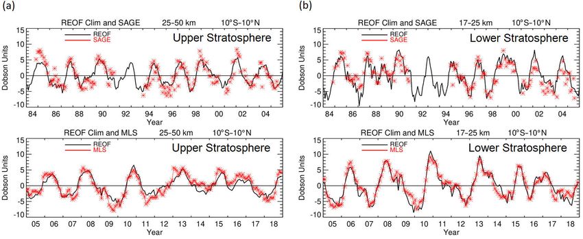
6408                               J. R. Ziemke et al.: A global ozone profile climatology for satellite retrieval algorithms

   We have generated a new ozone profile zonal-mean sea-         2     Ozone data and M2GMI model simulated ozone
sonal climatology (MLS/GMI) based on combining MLS
v4.2 and M2GMI ozone profiles which represents an im-            2.1    Aura MLS ozone
provement on our previous sonde–satellite ozone climatolo-
gies including ML. The earlier climatologies were binned in      The Microwave Limb Sounder (MLS) instrument onboard
10◦ latitude bands due mostly to the limited coverage of son-    the Aura spacecraft makes ozone profile measurements along
des. In contrast, the new MLS/GMI ozone profile climatol-        the orbital track during both daytime and nighttime. Aura is
ogy has been binned to 5◦ latitude bands by taking advan-        in a sun-synchronous orbit; therefore, MLS has nearly com-
tage of better spatial and temporal coverage of the model        plete latitudinal coverage each day between 82◦ S and 82◦ N,
output. This new climatology also extends to 80 km in al-        with local equatorial crossing times of approximately 13:45
titude compared with 65 km in the previous climatologies.        for the ascending sunlit portion of the orbit and 01:45 for the
The new MLS/GMI ozone profile climatology is provided            nighttime descending node.
for both volume mixing ratio (units of ppmv) and vertical           The MLS instrument is a thermal emission microwave
column concentration (Dobson units (DU) km−1 ).                  limb sounder that measures vertical profiles of mesospheric,
   We also generated a new interannual ozone profile cli-        stratospheric and upper tropospheric temperature, ozone and
matology based on MLS ozone, Solar Backscatter Ultra-            several other trace gases from limb scans made ahead of
Violet (SBUV) total ozone and rawinsonde wind data us-           Aura about 7 min before the satellite reaches the same point
ing a rotated empirical orthogonal function (REOF) method.       directly below. The MLS instrument primarily uses the
This REOF interannual climatology, just like the MLS/GMI         240 GHz microwave band for v4.2 ozone retrievals which,
seasonal climatology includes monthly zonal-mean profile         for recommended scientific applications, extend from 0.0215
ozone concentration (units DU km−1 ) within 5◦ latitude          to 261 hPa on 38 pressure layers. Vertical spacing for these
bands and altitudes from 0 to 80 km; however, the REOF cli-      layers is about 1.3 km everywhere below 1 hPa and about
matology represents a long time-dependent record beginning       2.7 km at most altitudes above 1 hPa. By comparison, the
in 1970 rather than a 12-month time record for the MLS/GMI       vertical resolution of the ozone retrievals is reported to be
climatology.                                                     ∼ 3 km extending from 261 hPa up into the mesosphere. Fur-
   The application of the MLS/GMI seasonal climatology           ther details regarding the MLS measurements are described
by itself or together with the REOF interannual climatology      by Livesey et al. (2011). The time record for the MLS ozone
as a priori enables more accurate profile and column ozone       used in our study was August 2004–December 2016. Given
retrievals, including improvements for inter-calibrating and     the high quality of MLS ozone in the low mesosphere, we
merging independent satellite ozone measurements such as         extend the climatology to 80 km from 65 km, where the ML
for the SBUV Merged Ozone Data Set (MOD) (Frith et al.,          climatology ended. We use only MLS measurements at the
2014). The REOF climatology has recently been used to            ascending part of the orbit with a local equatorial cross-
improve the calibration of long-record ozone measurements        ing time at ∼ 13:45. For most latitudes, this corresponds to
from ground Umkehr instruments (Irina Petropavlovskikh,          the daytime measurements (solar zenith angle < 90◦ ) from
personal communication, 2021) and from series of SBUV            MLS, as the daytime data are most appropriate for many pas-
instruments. The REOF climatology has also recently been         sive UV/Vis ozone remote sensing techniques that require
used to improve SBUV ozone profile retrievals by adding          daytime measurements. A number of studies of the diur-
interannual variability, which nadir instruments can not re-     nal ozone variations in stratospheric and mesospheric ozone
trieve due to a coarse vertical resolution. These SBUV ozone     (Parrish et al., 2014; Frith et al., 2020, and references therein)
profiles with improved interannual variability can be used for   have demonstrated sizable diurnal ozone variations around
the assimilated profile ozone records like one from the God-     5–10 hPa.
dard Modeling and Assimilation Office (GMAO) (Krzysztof
Wargan, personal communication, 2021).                           2.2    SBUV MOD total ozone record
   In the following sections, we describe the data and GMI
model output used in our analysis, outline the methods used      We use MOD total column ozone measurements from the So-
to construct the MLS/GMI seasonal climatology and REOF           lar Backscatter UltraViolet (SBUV) v8.6 retrievals as a proxy
climatology, and discuss the properties of the climatologies.    to reproduce time-dependent interannual variability for the
We conclude with a summary of our results. Additional de-        REOF climatology described in Sect. 4. The MOD total
tails and figures not covered in the main text are included in   ozone dataset (Frith et al., 2014) is comprised of a compos-
the Supplement.                                                  ite set of measurements from several SBUV instruments. The
                                                                 first instrument was Nimbus-4 BUV (Backscatter UltraVio-
                                                                 let) launched in 1970, followed by the second and improved
                                                                 version SBUV on Nimbus-7 launched in October 1978. Start-
                                                                 ing in 1989, seven SBUV/2 instruments were launched be-
                                                                 ginning with NOAA-9, followed by NOAA-11, -14, -16, -

Atmos. Meas. Tech., 14, 6407–6418, 2021                                            https://doi.org/10.5194/amt-14-6407-2021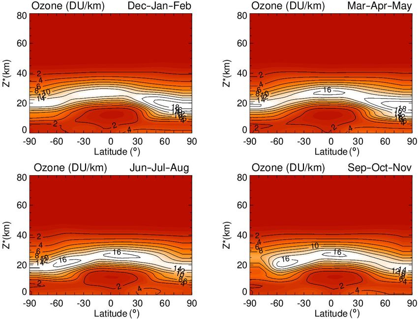
J. R. Ziemke et al.: A global ozone profile climatology for satellite retrieval algorithms                                 6409

17, -18 and -19. Currently, this record is extended with the      2.4     MERRA-2 GMI simulated ozone
Ozone Mapping and Profiler Suite (OMPS) Nadir Profiler
(NP) on board the Suomi National Polar-orbiting Partnership       The M2GMI simulation is produced with the Goddard Earth
(SNPP) satellite. There are four follow-up OMPS instrumen-        Observing System (GEOS) modeling framework (Molod et
tal suites as a part of the Joint Polar Satellite System (JPSS)   al., 2015), using winds, temperature and pressure from the
program (with JPSS-1/NOAA-20 already in operation) that           MERRA-2 reanalysis (Gelaro et al., 2017). The configura-
will extend the SBUV-type ozone observations over the next        tion for this study is a dynamically constrained replay (Orbe
2 decades. The SBUV instruments retrieve broad ozone pro-         et al., 2017) coupled to the Global Modeling Initiative (GMI)
files from measurements of backscattered solar UV radiation       stratospheric and tropospheric chemical mechanism (Dun-
which can be integrated to give total column ozone. All MOD       can et al., 2007; Oman et al, 2013; Nielsen et al., 2017).
instrument measurements have been processed using the v8.6        The simulation was run at ∼ 0.5◦ horizontal resolution, on
retrieval algorithm as described by McPeters et al. (2013) and    the cubed sphere, and output on the same 0.5◦ × 0.625◦ (lat-
Bhartia et al. (2013). In this study, we use monthly zonal-       itude × longitude) grid as MERRA-2 from 1980 to 2016. We
mean gridded total ozone extending from 90◦ S to 90◦ N at         refer to Strode et al. (2015, 2020) for details of the M2GMI
5◦ latitudinal binning (Stacey M. Frith, personal communi-        model simulation. The daily M2GMI ozone profiles were av-
cation, 2021). The MOD total ozone record spans from Jan-         eraged monthly and regridded from the original resolution to
uary 1970 to December 2020 with some temporal gaps, in-           zonal means in 5◦ latitude bands; the original 72 layers of the
cluding May 1976–October 1978 due to missing Nimbus-4             simulated profile ozone were also remapped to Z ∗ altitudes
BUV measurements.                                                 with 1 km vertical spacing (Sect. 3.2).

2.3   Ozonesonde measurements                                     2.4.1    Evaluation of M2GMI simulated tropospheric
                                                                           ozone
We include balloon-launched ozonesonde measurements for
comparison and validation of the M2GMI simulated tro-             Ozone profiles generated by the M2GMI simulation have
pospheric ozone. The used ozonesonde database extends             been extensively evaluated in a number of studies. Stauffer
from 2004 to 2019 and includes measurements from the              et al. (2019) provide a detailed global analysis of M2GMI
Southern Hemisphere ADditional OZonesondes (SHADOZ)               ozone profiles using comparisons with ozonesondes. On
program (Thompson et al., 2017; Witte et al., 2017), the          average, they found differences of about ±5 % between
World Ozone and Ultraviolet Data Center (WOUDC) (https:           M2GMI and sondes in the troposphere from 38 sonde sta-
//woudc.org/, last access: 23 September 2021) and the Net-        tions from 69◦ S to 79◦ N (their Fig. 1). The largest differ-
work for the Detection of Atmospheric Composition Change          ences were in the tropics where M2GMI was lower than
(NDACC) (http://www.ndsc.ncep.noaa.gov/, last access: 23          sonde by up to 10 %–20 % in low–mid troposphere, but
September 2021). The ozonesondes provide daily ozone pro-         M2GMI was higher than sonde by 40 %–50 % in the tropi-
file concentrations generally a few times per week as a func-     cal tropopause region; the large percentage differences, how-
tion of altitude; we include ozonesonde data from several         ever, can be due to relatively low mean background ozone
dozen global sites. Most of the sonde ozone profile measure-      concentrations of only ∼ 1–2 DU km−1 . Wargan et al. (2018)
ments that we use are from electrochemical concentration          compared the annual mean ozone mixing ratio anomalies for
cell (ECC) instruments. The sonde ozone profiles were inte-       1998–2016 between sondes and M2GMI at several stations
grated vertically each day from the surface to the tropopause     for 70, 100 and 200 hPa. Their comparisons show squared
to derive tropospheric column ozone (TCO) measurements            correlations varying from 0.62 to 0.93, and they concluded
using the same tropopause pressures as used for M2GMI             that the M2GMI simulation well captures the variability of
TCO. Tropopause pressure for both sonde and GMI TCO               tropospheric ozone including the upper troposphere–lower
was derived from National Centers for Environmental Pre-          stratosphere (UTLS) region. Ziemke et al. (2014) provide
diction (NCEP) reanalyses based on the World Meteorolog-          an additional evaluation of M2GMI tropospheric ozone by
ical Organization (WMO) 2 K km−1 temperature lapse-rate           comparing it with ozonesondes, satellite, and Global Model-
definition.                                                       ing and Assimilation Office (GMAO) data assimilation; the
   In Sect. 4, we describe construction of the REOF interan-      M2GMI and sonde daily comparisons from the tropics to
nual ozone profile climatology that includes monthly tropical     high latitudes in both hemispheres (their Figs. 2–7) showed
quasi-biennial oscillation (QBO) zonal winds. The tropical        offsets and standard deviations of differences varying ∼ 0–2
QBO zonal winds come from the Maldives (January 1970–             (∼ 0 %–7 %) and 4–7 DU (∼ 15 %–23 %), respectively. The
December 1975) and Singapore (January 1976–present) raw-          M2GMI simulated ozone profiles have also been extensively
insonde record (Free University of Berlin, https://www.geo.       compared with Atmospheric Tomography Mission (ATom)
fu-berlin.de/met/, last access: 23 September 2021).               aircraft flight measurements (Bourgeois et al., 2020) for the
                                                                  years 2015 and 2016 (Junhua Liu, personal communication,
                                                                  2020). The ATom in-flight measurements of the ozone vol-

https://doi.org/10.5194/amt-14-6407-2021                                           Atmos. Meas. Tech., 14, 6407–6418, 2021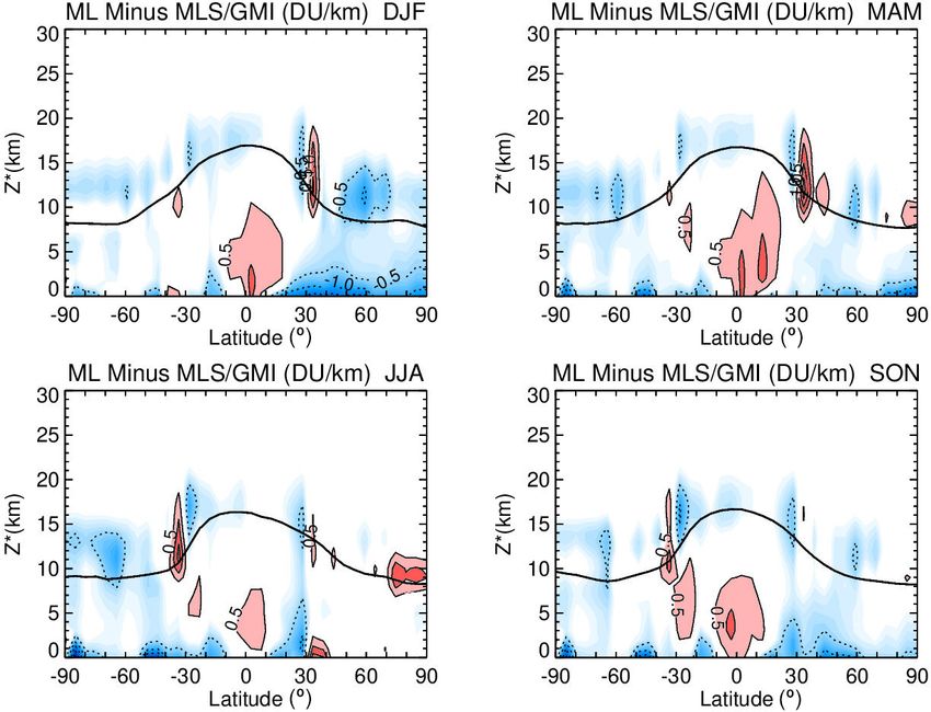
6410 J. R. Ziemke et al.: A global ozone profile climatology for satellite retrieval algorithms
ume mixing ratio are found to compare closely with M2GMI height Z ∗ = 5 km for climatological May. (Z ∗ is approxi-
simulated ozone, generally within about ±20 % along each mately equal to actual altitude and is defined in Sect. 3.2.)
of the mission flight paths that included meandering ascent Tropospheric ozone exhibits planetary-scale variability
and descent between the near-surface and tropopause each that includes a year-round zonal wave-1 pattern in the trop-
day. ics (greatest amplitude in September–October) and large-
Our study also includes the evaluation of M2GMI sim- scale patterns outside the tropics that vary greatly with sea-
ulated tropospheric ozone. Figure 1 compares sonde and son and region (Fishman et al., 1990). The tropical wave 1
M2GMI tropospheric column ozone (TCO) where the sonde in tropospheric ozone originates from regional sources of
and M2GMI measurements have been space–time co-located ozone: lightning, biofuel and biomass burning, stratosphere–
at the sonde station sites and seasonally averaged for 2004– troposphere exchange (STE), and transport associated with
2016. The co-location involved matching daily TCO from the the tropical east–west Walker circulation. In the extra-
sondes with M2GMI daily TCO at a 5◦ × 5◦ gridded resolu- tropics, the large planetary-scale features in tropospheric
tion interpolated to each sonde latitude–longitude location. ozone have a strong seasonal dependence, with the seasonal
As noted in Sect. 2.3, both daily sonde and M2GMI TCO maximum in JJA in the NH and SON (September–October–
were derived using the same NCEP WMO tropopause pres- November) in the Southern Hemisphere (SH). These sea-
sures. sonal patterns in tropospheric ozone outside the tropics are
The M2GMI ozone in Fig. 1 closely simulates the sonde also due to the combined effects of STE, biofuel, light-
ozone year-round with an exception in the Northern Hemi- ning, biomass burning and long-range transport. The global
sphere (NH) mid–high latitudes in MAM (March–April– planetary-scale patterns in tropospheric ozone columns were
May) and JJA (June–July–August) where the simulation first shown from TOMS/SAGE (Fishman et al., 1990) and
tends to underdetermine sonde TCO by ∼ 5 DU or more. TOMS/MLS (Ziemke et al., 1996) satellite measurements.
Section S3 in the Supplement includes additional discussion The patterns in the M2GMI tropospheric ozone mixing ra-
and figures regarding the evaluation of M2GMI tropospheric tio for Z ∗ = 5 km in Fig. 2 in the tropics and in the NH are
ozone profiles using ozonesondes and surface lidar measure- similar to the TCO May pattern from satellite records.
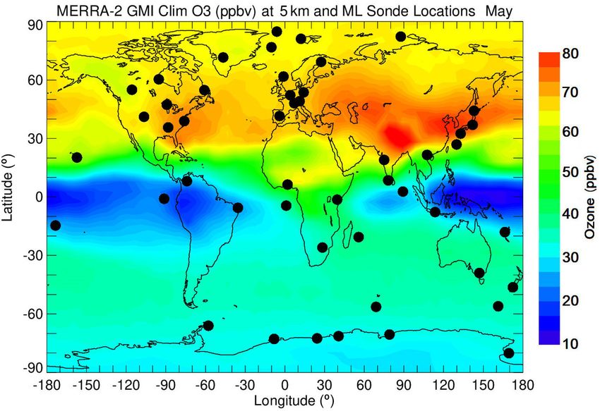
ments. It is apparent from Fig. 2 that the ensemble of ozoneson-
des is unlikely to effectively represent the zonal-mean tro-
pospheric ozone values due to their limited sampling. For
example, the sonde measurements undersample the tropical
3 The MLS/GMI seasonal climatology wave-1 structure in tropospheric ozone in the tropics. Due
to the undersampling in the tropical Pacific area, sondes do
The MLS/GMI seasonal climatology product is derived for not capture the very low ozone concentrations of ∼ 10 ppbv.
both volume mixing ratio (units ppmv) and vertical column This leads to the overestimation of zonal-mean tropospheric
concentration (DU km−1 ); the latter has vertical and latitudi- ozone in the tropics from the sondes. We will show later that
nal structure that is closely similar to that of ozone number this overdetermination of ML tropospheric ozone in the trop-
density and ozone partial pressure. Standard deviations are ics averages to about 5–10 DU in TCO year-round between
reported for both mixing ratios and column concentrations 20◦ S and 20◦ N. The sondes also tend to miss the high val-
based upon all available daily ozone profiles over a given ues of ozone in the NH midlatitudes over the Asian continent
month and within every 5◦ latitude band. The standard devi- (see Fig. 2), thereby introducing a low bias in zonal-mean
ations provide a measure of climatological ozone variability tropospheric ozone in NH midlatitudes.
and are important for error covariance matrices included as a
priori information in retrieval algorithms such as the optimal 3.2 Merging MLS and M2GMI ozone profiles
estimation method of Rodgers (2000). We refer the reader to
the Supplement for further discussion and figures involving Simulated ozone volume mixing ratio values from the
calculated standard deviations. M2GMI model were merged with ozone volume mixing ratio
measurements from MLS to construct the ozone profile sea-
3.1 Global coverage of M2GMI tropospheric ozone sonal climatology in the format of monthly zonal means. The
compared with sondes merging of MLS and M2GMI ozone involved monthly zonal-
mean ozone profiles for both records in 5◦ latitude bands
Our motivation for using M2GMI simulation data is that they with Z ∗ altitudes of 0–80 km (1 km increments). For low lati-
provide a better spatial and temporal representation of tro- tudes and midlatitudes between 40◦ N and 40◦ S, the M2GMI
pospheric ozone profiles than ozonesondes. The sondes are and MLS profiles were merged for Z ∗ levels between 13
sparsely distributed over the Earth with generally only a few and 21 km (156 to 49 hPa). For latitudes poleward of 40◦ in
measured profiles per month for a given station. The lim- each hemisphere, the profiles were merged slightly lower in
ited spatial coverage of sondes is demonstrated in Fig. 2 with the atmosphere, for Z ∗ levels between 8 and 16 km (320 to
the M2GMI mid-tropospheric ozone concentration (ppbv) at 101 hPa). Within the merged altitude ranges the climatology
Atmos. Meas. Tech., 14, 6407–6418, 2021 https://doi.org/10.5194/amt-14-6407-2021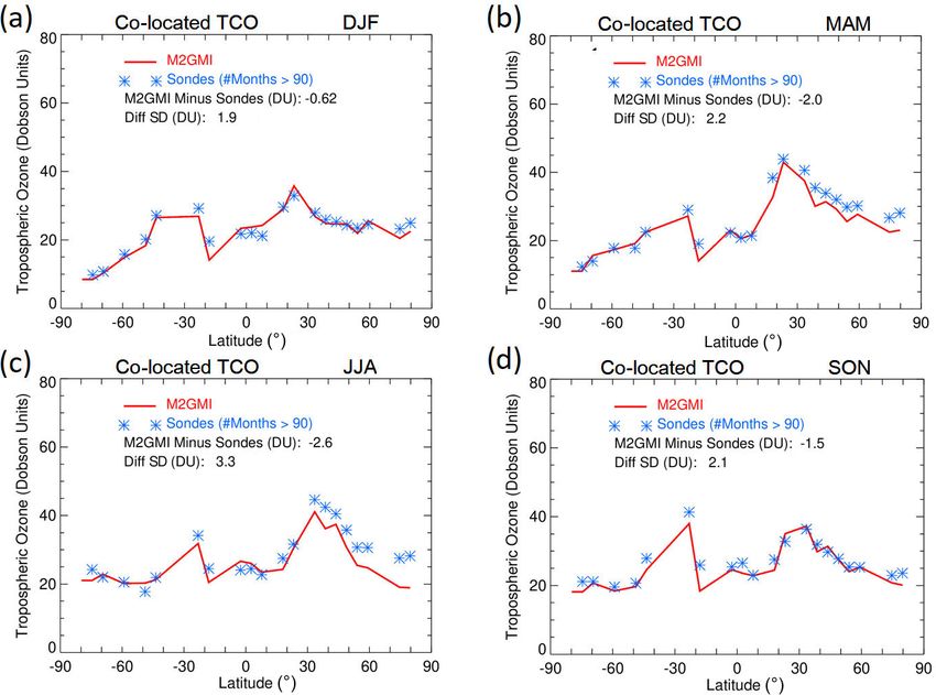
J. R. Ziemke et al.: A global ozone profile climatology for satellite retrieval algorithms                                    6411

Figure 1. Comparisons between M2GMI simulated (red curves) and ozonesonde (blue asterisks) TCO averaged over 3-month seasons
(indicated) for 2004–2016. The M2GMI TCO field is sampled daily at the sonde station locations. All TCO is in Dobson units (DU).
The same daily tropopause is used for both M2GMI and sonde to derive TCO, and it is defined according to the WMO 2 K km−1 lapse-
rate tropopause definition using NCEP temperatures. Included in each panel are mean offsets and standard deviations of TCO seasonal
differences.

                                                                     is weighted linearly, from 100 % M2GMI at the lowest alti-
                                                                     tude to 100 % MLS at the highest altitude. Standard devia-
                                                                     tions were calculated for each climatological ozone value.
                                                                        As in previous climatologies, the altitude variable used for
                                                                     our climatology is Z ∗ , a parameter frequently used in com-
                                                                     parisons of atmospheric chemistry models (Park et al., 1999).
                                                                     Z ∗ is in units of kilometers but can be considered a pressure
                                                                     variable. Z ∗ (km) is defined by Z ∗ = 16·log(1013/P ), where
                                                                     P is atmospheric pressure (in hPa). The altitude spacing for
                                                                     our climatology is 1 km in Z ∗ units. In an isothermal terres-
                                                                     trial atmosphere, Z ∗ would correspond closely to altitude.

                                                                     3.3   Comparisons with the ML climatology

                                                                     We first examine basic global patterns of the MLS/GMI
Figure 2. Map of climatological ozone volume mixing ratio (in        seasonal climatology. Figure 3 shows vertical column con-
ppbv) from the M2GMI simulation at Z ∗ = 5 km altitude (see          centrations (DU km−1 ) for the climatology by 3-month sea-
Sect. 3.2) for the month of May. Blue color indicates areas with     son (indicated) for Z ∗ = 0–80 km. Column concentrations in
an ozone concentration of about 10 ppbv, and red color corresponds   the low stratosphere in both hemispheres are largest during
to regions with > 75 ppbv. Black circles show the locations of the   winter–spring and smallest in summer. In both hemispheres,
sonde stations with a long observational record. Data from these
                                                                     ozone is largest in the winter–spring months due to seasonal
stations were used to constrain tropospheric ozone profiles in the
                                                                     transport from the tropics to the extra-tropics during this pe-
ML climatology.
                                                                     riod (i.e., the Brewer–Dobson circulation) and longer life-
                                                                     times for ozone in the low stratosphere. The highest ozone
                                                                     amounts in Fig. 3 are ∼ 18–20 DU km−1 in the NH around

https://doi.org/10.5194/amt-14-6407-2021                                              Atmos. Meas. Tech., 14, 6407–6418, 2021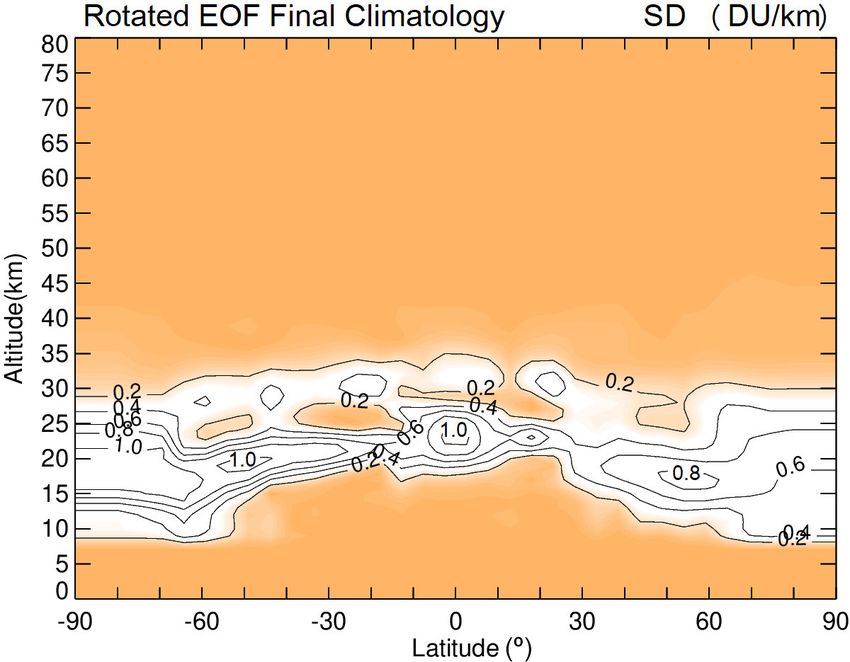
6412                                J. R. Ziemke et al.: A global ozone profile climatology for satellite retrieval algorithms

20 km during winter and spring. In the troposphere, very low       in both the troposphere and stratosphere. However, interan-
ozone density of less than 2 DU km−1 occurs in the tropics         nual processes such as the QBO produce sizable changes in
year-round.                                                        the vertical ozone distribution in stratospheric ozone from
   While the basic characteristics of stratospheric ozone in       year to year. To capture these variations, we have constructed
Fig. 3 are important to note, our main focus is to compare         a global time-dependent climatology of stratospheric ozone
tropospheric ozone in Fig. 3 with the ML sonde ozone cli-          that represents ozone interannual variability. This clima-
matology. Because the ML climatology uses sparsely sam-            tology can be used either independently or added to the
pled sonde measurements to estimate zonal means in the tro-        MLS/GMI seasonal climatology, depending on the particu-
posphere, it is possible that there may be substantial differ-     lar application.
ences.                                                                The derivation of the interannual ozone climatology is
   Figure 4 shows the difference between ML and MLS/GMI            lengthy and is discussed in detail in the Supplement. In this
zonal-mean profile ozone by season, plotted as Z ∗ altitude        section, we provide only a short overview of the method-
versus latitude. Only Z ∗ levels 0–30 km are included in Fig. 4    ology and discuss the final product. The interannual ozone
to highlight differences in ozone profiles used for the tropo-     climatology is constructed using a method that includes an
sphere and the low stratosphere merging region. Year-round         REOF analysis as described by Richman (1986, and ref-
positive differences in the tropics in Fig. 4 suggest that ML      erences therein). With our approach, vertical information
is always too large in the low–mid troposphere compared            for the climatology comes from an REOF analysis of MLS
with M2GMI due to the absence of ML sonde measurements             ozone profiles, while month-to-month time dependence fol-
in the Pacific region where tropospheric ozone is low (e.g.,       lows by coupling the REOF analysis time coefficients with
Fig. 2). At latitudes around ±35◦ and elsewhere in the low         SBUV MOD total ozone and tropical QBO zonal winds.
stratosphere merging region in Fig. 4, there are anomalous         The time period for the REOF climatology depends on the
differences from −0.5 up to +1.5 DU km−1 ; these sharp pat-        availability of total ozone and tropical QBO winds. The time
terns are ascribed to sonde sampling issues for the ML cli-        period for this climatology is 1970–2018 (588 consecutive
matology. In the boundary layer throughout the NH extra-           months) with gaps present due to some missing MOD to-
tropics during winter (i.e., upper-left panel in Fig. 4), the      tal ozone including Nimbus-4 measurements in the 1970s.
M2GMI ozone is higher than sondes by ∼ 0.5 to 1 DU km−1 .          We plan to periodically extend this REOF climatology when
These latter differences are attributed to a known model issue     zonal wind and MOD total ozone data become available.
related to underestimating surface deposition over cold sur-       Before applying the REOF approach, an empirical orthog-
faces (Jaegle et al., 2018), which is most prominent in the NH     onal function (EOF) method (Kutzbach, 1967, and refer-
boundary layer during winter. When compared with ML in             ences therein) was applied to MLS ozone anomaly profiles
Fig. 4, the model in this region overdetermines the ozone col-     to derive repeatable interannual patterns in the ozone vertical
umn in DJF (December–January–February) by about 2 DU.              distribution; that is, the EOF analysis was applied to MLS
   Line plots of seasonal differences (ML minus MLS/GMI)           monthly zonal-mean ozone profile anomalies derived by re-
of integrated ozone columns are shown in Fig. 5 for 0–8 km         moving seasonal cycles between August 2004 and Decem-
(Fig. 5a) and 0–16 km (Fig. 5b). These line plots are deter-       ber 2016. All MLS ozone and anomaly ozone profiles were
mined from Fig. 4 by summing the 1 km layers of ML mi-             binned into 5◦ latitude bands (36 bands for 90◦ S–90◦ N, sim-
nus MLS/GMI differences. In the tropics, the 0–16 km in-           ilar to MLS/GMI climatology) between 1 and 261 hPa (30
tegrated column in Fig. 5b represents the total troposphere        pressure levels).
(i.e., TCO) with ML larger than MLS/GMI by about 10 DU                The main challenge of EOF analysis is interpretation of
year-round. Comparison with the 0–8 km columns in Fig. 5a          derived EOFs and EOF time coefficients and their attribu-
shows that these differences in the tropics originate mostly       tion to specific geophysical processes. As described in the
from the lower troposphere, which is consistent with all four      Supplement, the construction of this REOF climatology re-
panels in Fig. 4. Outside the tropics in Fig. 5, there are sea-    quired only total ozone and tropical stratospheric zonal wind
sonal offset differences in the NH of up to −5 to −10 DU           time series to explain most of the stratospheric ozone pro-
during DJF. Part of the reason for the ML minus MLS/GMI            files variability (total EOF variance). We used MLS ozone
biases in Fig. 5 is sonde undersampling for the ML climatol-       anomalies expressed as ozone partial pressure for the REOF
ogy, particularly in the tropics, as noted for Fig. 4. The sonde   analysis rather than ozone mixing ratio because it helped to
undersampling also creates the sharp (nonphysical) variabil-       attribute the REOF-1 time coefficient directly to total ozone
ity seen between adjacent latitude bins in Fig. 5.                 column measurements at all latitudes. The first REOF vec-
                                                                   tor with the MOD total ozone time series as a proxy explains
                                                                   about 50 %–70 % of the interannual ozone variability. Next,
4   An interannual ozone profile climatology                       we derived a second REOF-2 that we attributed to the QBO
                                                                   and used the equatorial zonal wind time series as a proxy
The MLS/GMI seasonal climatology captures the vertical             for REOF-2. The sum of these two REOFs explains about
shape of zonal-mean ozone profiles by season and latitude          70 %–80 % of the interannual variability in deseasonalized

Atmos. Meas. Tech., 14, 6407–6418, 2021                                             https://doi.org/10.5194/amt-14-6407-2021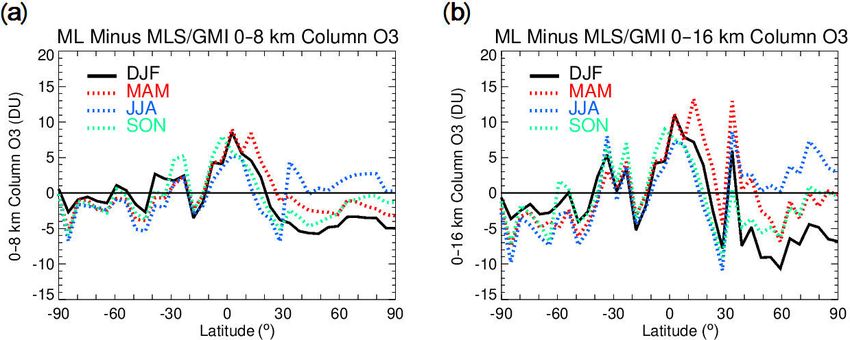
J. R. Ziemke et al.: A global ozone profile climatology for satellite retrieval algorithms                                          6413

Figure 3. Meridional cross sections of derived zonal-mean vertical ozone concentration (units DU km−1 ) for the MLS/GMI seasonal clima-
tology. This 12-month climatology is averaged over 3-month seasons (indicated) for 2004–2016 and is binned for 5◦ latitude bands and Z ∗
levels from 0 to 80 km at 1 km spacing (see text).

Figure 4. Meridional cross sections of ML minus MLS/GMI climatologies of ozone column concentration (DU km−1 ). These differences
are averaged over 3-month seasons (indicated) for 2004–2016 and are binned for 10◦ latitude bands and Z ∗ levels from 0 to 30 km at 1 km
spacing. Contour levels (indicated) are at 0.5 DU km−1 increments: blue and dashed contours mean negative, and pink and red solid contours
mean greater than 0.5 DU km−1 . The black line indicates tropopause height according to the WMO 2 K km−1 lapse-rate tropopause definition
using NCEP temperatures. White color denotes zero differences.

https://doi.org/10.5194/amt-14-6407-2021                                                  Atmos. Meas. Tech., 14, 6407–6418, 2021
6414                                J. R. Ziemke et al.: A global ozone profile climatology for satellite retrieval algorithms

Figure 5. (a) Line plots of seasonal differences of ML minus MLS/GMI integrated ozone columns for 0–8 km. The differences are averaged
over 3-month seasons (indicated by DJF, MAM, JJA and SON). Panel (b) is the same as panel (a) but for 0–16 km ozone columns.

MLS zonal-mean ozone profiles. As only MLS profiles are
used to constrain the vertical shapes of the REOFs and time
coefficients are described by total ozone and zonal winds,
this REOF climatology can be used in the future (even after
MLS stops operating) or can be extended into the past to the
pre-Aura time period whenever total column ozone and wind
data are available.
   The REOF climatology was finally converted from the
ozone partial pressures defined at 30 MLS levels to volume
mixing ratio (ppmv) and partial ozone column (DU km−1 )
at the 1 km Z ∗ levels (defined in Sect. 3.2) identical to the
MLS/GMI climatology. The REOF climatological values at
levels below ∼ 9 km and above ∼ 48 km are very small in
contributing to interannual variability of ozone and are set
to zero. As the REOF climatology uses zonal wind and total
ozone time series that can have long-term trends, we applied
a very low frequency (VLF) digital low-pass filter to the fi-
nal derived REOF climatology to remove long-term decadal             Figure 6. Temporal standard deviation (in DU km−1 ) for 1970–
                                                                     2018 for the final REOF ozone climatology (i.e., Eq. S10 in the Sup-
variability. This was done to ensure that the climatology
                                                                     plement). The interannual variability in the tropical low latitudes is
captures only interannual variability in monthly zonal-mean
                                                                     almost entirely due to the QBO. Interannual variability in the extra-
ozone anomaly profiles without inducing decadal trends if            tropics comes from the QBO coupled with other non-QBO-related
used as a priori in ozone retrieval. The frequency response          interannual variability.
of the applied VLF digital filter (Stanford et al., 1993) is ex-
actly 0.0 (1.0) at zero (Nyquist) frequency with an amplitude
of 0.5 at a frequency of 0.00333 per month; the filter was also
designed to have zero phase shift at all frequencies.                not do nearly as well at resolving vertical changes in strato-
   We demonstrate that the REOF climatology does very well           spheric ozone.
in capturing interannual variability of monthly zonal-mean              The magnitude of interannual variability in profile ozone,
stratospheric ozone. The high vertical resolution of MLS             captured by the REOF climatology, is shown in Fig. 6 as cal-
ozone limb measurements of ∼ 3 km resolves much of the               culated standard deviations (in DU km−1 ) for the 1970–2018
vertical variability of ozone caused by low-frequency and            period. In the tropical low latitudes from 10◦ S to 10◦ N, the
episodic processes such as the QBO, extra-tropical strato-           main source of interannual variability is the QBO. However,
spheric warmings and other year-round planetary-scale wave           larger interannual variability occurs in the SH extra-tropics
events (e.g., Ziemke et al., 2014, and references therein).          due to the QBO and additional dynamical sources. In an ef-
Many nadir instrument ozone profile retrievals have coarse           fort to understand the contribution of non-QBO processes
vertical resolution of ∼ 6 to 10 km or greater (such as from         to the interannual variability, we also generated a climatol-
SBUV or the Ozone Monitoring Instrument, OMI) and can-               ogy using only equatorial QBO zonal winds as a proxy (see
                                                                     Fig. S4 in the Supplement). When compared with the REOF
                                                                     climatology in Fig. 6, only a very small fraction of interan-

Atmos. Meas. Tech., 14, 6407–6418, 2021                                                 https://doi.org/10.5194/amt-14-6407-2021
J. R. Ziemke et al.: A global ozone profile climatology for satellite retrieval algorithms 6415
Figure 7. (a) The top panel is zonal-mean upper-stratospheric column ozone (in Dobson units) for the REOF climatology (black curve)
and deseasonalized SAGE II (red asterisks) spanning from 1984 to 2005 and averaged between 10◦ S and 10◦ N. The SAGE data are
deseasonalized monthly zonal means. All column amounts are calculated by integrating ozone profiles for Z ∗ = 25–50 km (∼ 28 to 1 hPa).
The bottom panel is the same as the top panel but with MLS in place of SAGE and for the time period from 2005 to 2018. The panels in (b)
are the same as those in (a) but for the lower stratosphere with Z ∗ = 17–25 km (∼ 88 to 28 hPa).
nual variability is captured in the extra-tropics for the QBO- 5 Summary
only climatology.
The long record of the REOF interannual ozone profile cli-
We have produced a new MLS/GMI seasonal ozone profile
matology has been compared with deseasonalized ozone pro-
climatology by combining ozone profiles from the M2GMI
file measurements from SAGE II and Aura MLS for 1984–
model simulation with MLS v4.2 measurements. M2GMI is
2018 (Fig. 7). The top panel in Fig. 7a shows comparisons
used primarily for tropospheric ozone and MLS for strato-
of upper-stratospheric column ozone anomalies (Z ∗ = 25–
spheric ozone, with the two ozone profile datasets blended
50 km) between REOF (black curve) and SAGE (red aster-
together in the low stratosphere; the result is a merged zonal-
isks) for the years from 1984 to 2005 in the tropics (10◦ S–
mean 12-month global ozone profile climatology at a 5◦
10◦ N). The bottom panel in Fig. 7a shows a similar compari-
latitudinal resolution with a Z ∗ altitude range of 0–80 km
son between REOF and MLS for 2005–2018. Figure 7b is the
(1 km vertical sampling). Our main interest in generating the
same as in Fig. 7a but for the lower stratosphere (Z ∗ = 17–
MLS/GMI climatology is to use it as a priori information in
25 km).
satellite ozone retrieval algorithms. However, it is also use-
The SAGE II sampling of ozone columns in Fig. 7 is
ful as a baseline for evaluating various modeled or measured
sparse, averaging ∼ 2–3 d of measurements for a given
ozone seasonal and interannual variability, and in studies in-
month in the 10◦ S–10◦ N latitude band shown. This means
volving corresponding ozone radiative forcing as inferred
that the monthly SAGE measurements in Fig. 7 are more
from atmospheric radiative transfer calculations.
representative of daily profiles than monthly means. Ozone
In previous studies, we generated several ozone profile
profiles on a daily basis in the tropics are distorted by propa-
climatologies based on combining ozonesondes with either
gating tropical waves with periods of days to weeks such as
SAGE or MLS satellite measurements (e.g., McPeters et
Kelvin waves, equatorial Rossby waves and mixed Rossby–
al., 2007; McPeters and Labow, 2012; Labow et al., 2015).
gravity waves (e.g., Timmermans et al., 2005; Ziemke
We have compared the new MLS/GMI climatology in detail
and Stanford, 1994). As a result, the upper- and lower-
with the ML climatology (of McPeters and Labow, 2012)
stratospheric columns in Fig. 7 for SAGE II will have noisy
that used ozonesondes for tropospheric ozone profiles. The
month-to-month variations of several Dobson units because
M2GMI model simulation provides an improved ozone cli-
of these tropical waves. The Supplement includes further dis-
matology for the troposphere compared with the ML clima-
cussion and more figures relating to the REOF climatology.
tology due to the fact that it has much better spatial and tem-
poral coverage than the sondes.
We also developed a time-dependent climatology of
monthly zonal-mean profile ozone anomalies representing
https://doi.org/10.5194/amt-14-6407-2021 Atmos. Meas. Tech., 14, 6407–6418, 20216416 J. R. Ziemke et al.: A global ozone profile climatology for satellite retrieval algorithms
interannual variability. This interannual climatology was opment of the MLS/GMI seasonal climatology and providing the
constructed using a rotational EOF analysis of Aura MLS ozonesonde database used for validation. NAK also helped to write
monthly zonal-mean profile ozone anomalies from August the paper and was responsible for the analyses of total ozone and
2004 to December 2016 within each 5◦ latitude band. The tropospheric ozone, and the derived climatologies. RDM and PKB,
analysis shows that the first two leading EOFs explain ∼ as experts on ozone algorithms, contributed to the analysis that in-
cluded their extensive experience in developing ozone climatolo-
70 %–80 % of interannual variability of profile ozone at all
gies and applications involving the rotational EOF technique. LDO
latitudes. Furthermore, total ozone and tropical zonal wind helped with the analysis and writing the paper, especially regard-
time series correlate well with the two leading EOF coeffi- ing the M2GMI simulated ozone. SMF and DPH played key roles
cient time series and were used as proxies to extend infor- involving the analysis of the derived seasonal and REOF climatolo-
mation outside the Aura MLS time range. We used these re- gies.
lationships to reconstruct anomalies at a 5◦ latitudinal reso-
lution for Z ∗ = 0–80 km and 1970–2018. This REOF time-
dependent climatology was compared to a similar climatol- Competing interests. The contact author has declared that neither
ogy based on only tropical QBO winds. The advantage of they nor their co-authors have any competing interests.
the REOF climatology is that it allows for a much more thor-
ough representation of interannual variability of stratospheric
ozone than just the QBO. Disclaimer. Publisher’s note: Copernicus Publications remains
The REOF time-dependent climatology of ozone profile neutral with regard to jurisdictional claims in published maps and
anomalies can be easily added to the MLS/GMI seasonal cli- institutional affiliations.
matology to simulate both seasonal and interannual variabil-
ity of stratospheric ozone. We note that both the MLS/GMI
12-month climatology and the REOF climatology were gen- Acknowledgements. We thank the NASA Jet Propulsion Labora-
tory MLS team for the MLS v4.2 ozone dataset, and the SHADOZ,
erated using Aura time period MLS ozone measurements,
WOUDC and NDACC personnel for providing the extensive
and neither of them account for long-term trends in strato- ozonesonde measurements that we used for our study. We also thank
spheric ozone. the NASA MAP program for supporting the MERRA-2 GMI sim-
ulation and the NASA Center for Climate Simulation (NCCS) for
providing high-performance computing resources. Special thanks
Code availability. Codes used to generate the ozone climatologies go to the NASA GMI group, especially Sarah Strode, regarding the
along with the analyses in this study are available upon personal MERRA-2 GMI simulation.
request to Jerald R. Ziemke (jerald.r.ziemke@nasa.gov).
Financial support. This research has been supported by the NASA
Data availability. The data description for MLS v4.2 ozone and programmatic fund “Long-term ozone trends” (project no. WBS
links to the data can be obtained from the following web- 479717). Jerald R. Ziemke and Natalya A. Kramarova were also
sites: https://mls.jpl.nasa.gov/ (NASA MLS division, 2021) and supported by the NASA ROSES proposal “Improving total and
https://disc.gsfc.nasa.gov/ (NASA MLS science research group, tropospheric ozone column products from EPIC on DSCOVR for
2021). The MERRA-2 GMI model description and access are studying regional scale ozone transport” (grant no. 18-DSCOVR18-
available from https://acd-ext.gsfc.nasa.gov/Projects/GEOSCCM/ 0011, DSCOVR Science Team). Gordon J. Labow, Stacey M. Frith
MERRA2GMI/ (Code 614 GMI modeling group, 2021). The MOD and David P. Haffner were supported under NASA contract
total ozone measurements are available from https://acd-ext.gsfc. NNG17HP01C. Luke D. Oman was supported by the NASA “Mod-
nasa.gov/Data_services/merged/ (Code 614 ozone trends group, eling, Analysis, and Prediction” (MAP) program.
2021). Tropical QBO winds were provided by the Free University of
Berlin (2021): https://www.geo.fu-berlin.de/met/ag/strat/produkte/
qbo/qbo.dat. The seasonal and interannual climatology products de- Review statement. This paper was edited by Mark Weber and re-
rived from our study are available for the general public using the viewed by two anonymous referees.
direct links on the NASA website: https://avdc.gsfc.nasa.gov/ (last
access: 23 September 2021).
References
Supplement. The supplement related to this article is available on-
line at: https://doi.org/10.5194/amt-14-6407-2021-supplement. Bhartia, P. K., McPeters, R. D., Flynn, L. E., Taylor, S., Kramarova,
N. A., Frith, S., Fisher, B., and Deland, M.: Solar Backscatter UV
(SBUV) total ozone and profile algorithm, Atmos. Meas. Tech.,
Author contributions. JRZ is the lead author of the paper and was 6, 2533–2548, https://doi.org/10.5194/amt-6-2533-2013, 2013.
responsible for writing the paper and data analysis that included the Bourgeois, I., Peischl, J., Thompson, C. R., Aikin, K. C., Campos,
development of the REOF interannual climatology and validation. T., Clark, H., Commane, R., Daube, B., Diskin, G. W., Elkins,
GJL helped to write the paper and was responsible for the devel- J. W., Gao, R.-S., Gaudel, A., Hintsa, E. J., Johnson, B. J., Kivi,
Atmos. Meas. Tech., 14, 6407–6418, 2021 https://doi.org/10.5194/amt-14-6407-2021J. R. Ziemke et al.: A global ozone profile climatology for satellite retrieval algorithms 6417 R., McKain, K., Moore, F. L., Parrish, D. D., Querel, R., Ray, pro?le climatology based on ozonesondes and Aura E., Sánchez, R., Sweeney, C., Tarasick, D. W., Thompson, A. MLS data, J. Geophys. Res.-Atmos., 120, 2537–2545, M., Thouret, V., Witte, J. C., Wofsy, S. C., and Ryerson, T. https://doi.org/10.1002/2014JD022634, 2015. B.: Global-scale distribution of ozone in the remote troposphere Livesey, N. J., Read, W. G., Froidevaux, L., Lambert, A., Manney, from the ATom and HIPPO airborne field missions, Atmos. G. L., Pumphrey, H. C., Santee, M. L., Schwartz, M. J., Wang, S., Chem. Phys., 20, 10611–10635, https://doi.org/10.5194/acp-20- Cofield, R. E., Cuddy, D. T., Fuller, R. A., Jarnot, R. F., Jiang, J. 10611-2020, 2020. H., Knosp, B. W., Stek, P. C., Wagner, P. A., and Wu, D. L.: EOS Code 614 GMI modeling group: MERRA-2 GMI model results, MLS Version 3.3 Level 2 data quality and description document, NASA Goddard Space Flight Center, available at: https://acd-ext. Tech. Rep., Jet Propulsion Laboratory, available at: http://mls.jpl. gsfc.nasa.gov/Projects/GEOSCCM/MERRA2GMI/, last access: nasa.gov/ (last access: 23 September 2021), 2011. 16 April 2021. McPeters, R. D. and Labow, G. J.: Climatology 2012: Code 614 ozone trends group: MOD total ozone dataset, Goddard An MLS and sonde derived ozone climatology for Space Flight Center, available at: https://acd-ext.gsfc.nasa.gov/ satellite retrieval algorithms, J. Geophys. Res., 117, Data_services/merged/, last access: September 2021. https://doi.org/10.1029/2011JD017006, 2012. Duncan, B. N., Strahan, S. E., Yoshida, Y., Steenrod, S. D., and McPeters, R. D., Labow, G. J., and Logan, J. A.: Ozone climatolog- Livesey, N.: Model study of the cross-tropopause transport of ical profiles for satellite retrieval algorithms, J. Geophys. Res., biomass burning pollution, Atmos. Chem. Phys., 7, 3713–3736, 112, D05308, https://doi.org/10.1029/2005JD006823, 2007. https://doi.org/10.5194/acp-7-3713-2007, 2007. McPeters, R. D., Bhartia, P. K., Haffner, D., Labow, G. Fishman, J., Watson, C. E., Larsen, J. C., and Logan, J. A.: Distri- J., and Flynn, L.: The version 8.6 SBUV ozone data bution of tropospheric ozone determined from satellite data, J. record: An overview, J. Geophys. Res., 118, 8032–8039, Geophys. Res., 95, 3599–3617, 1990. https://doi.org/10.1002/jgrd.50597, 2013. Free University of Berlin: Tropical QBO zonal, available Molod, A., Takacs, L., Suarez, M., and Bacmeister, J.: Development at: https://www.geo.fu-berlin.de/met/ag/strat/produkte/qbo/qbo. of the GEOS-5 atmospheric general circulation model: evolution dat, last access: 23 September 2021. from MERRA to MERRA2, Geosci. Model Dev., 8, 1339–1356, Frith, S. M., Kramarova, N. A., Stolarski, R. S., McPeters, R. https://doi.org/10.5194/gmd-8-1339-2015, 2015. D., Bhartia, P. K., and Labow, G. J.: Recent changes in to- NASA MLS division: MLS data, JPL, available at: https://mls.jpl. tal column ozone based on the SBUV Version 8.6 Merged nasa.gov/, last access 23 September 2021. Ozone Data Set, J. Geophys. Res.-Atmos., 119, 9735–9751, NASA MLS science research group: MLS data, NASA Goddard https://doi.org/10.1002/2014JD021889, 2014. Space Flight Center, available at: https://disc.gsfc.nasa.gov/, last Frith, S. M., Bhartia, P. K., Oman, L. D., Kramarova, N. access: 16 April 2021. A., McPeters, R. D., and Labow, G. J.: Model-based cli- Nielsen, J. E., Pawson, S., Molod, A., Auer, B., da Silva, A. M., matology of diurnal variability in stratospheric ozone as Douglass, A. R., Duncan, B. N., Liang, Q., Manyin, M., Oman, a data analysis tool, Atmos. Meas. Tech., 13, 2733–2749, L., D., Putman, W., Strahan, S. E., and Wargan, K.: Chemical https://doi.org/10.5194/amt-13-2733-2020, 2020. mechanisms and their applications in the Goddard Earth Observ- Gelaro, R., McCarty, W., Suárez, M. J., Todling, R., Molod, A., ing System (GEOS) earth system model, J. Adv. Model. Earth Takacs, L., Randles, C. A., Darmenov, A., Bosilovich, M. G., Re- Syst., 9, 3019–3044, https://doi.org/10.1002/2017MS001011, ichle, R., Wargan, K., Coy, L., Cullather, R., Draper, C., Akella, 2017. S., Buchard, V., Conaty, A., da Silva, A. M., Gu, W., Kim, G., Oman, L. D., Douglass, A. R., Ziemke, J. R., Rodriguez, Koster, R., Lucchesi, R., Merkova, D., Nielsen, J. E., Partyka, J. M., Waugh, D. W., and Nielsen, J. E.: The ozone re- G., Pawson, S., Putman, W., Rienecker, M., Schubert, S. D., sponse to ENSO in Aura satellite measurements and a Sienkiewicz, M., and Zhao, B.: The Modern-Era Retrospective chemistry-climate simulation, J. Geophys. Res., 118, 965–976, Analysis for Research and Applications, Version 2 (MERRA-2), https://doi.org/10.1029/2012JD018546, 2013. J. Climate, 30, 5419–5454, https://doi.org/10.1175/JCLI-D-16- Orbe, C., Oman, L. D., Strahan, S. E., Waugh, D. W., Pawson, 0758.1, 2017. S., Takacs, L. L., and Molod, A. M.: Large-Scale Atmospheric Jaeglé, L., Shah, V., Thornton, J. A., Lopez-Hilfiker, F. D., Lee, B. Transport in GEOS Replay Simulations, J. Adv. Model. Earth H., McDuffie, E. E., Fibiger, D., Brown, S. S., Veres, P., Sparks, Sy., 9, 2545–2560, 2017. T. L., Ebben, C. J., Wooldridge, P. J., Kenagy, H. S., Cohen, Park, J. H., Ko, M. K., Jackman, C. H., Plumb, R. A., Kaye, J. A., R. C., Weinheimer, A. J., Campos, T. J., Montzka, D. D., Di- and Sage, K. H.: Models and Measurements Intercomparison II, gangi, J. P., Wolfe, G. M., Hanisco, T., Schroder, J. C., and Cam- NASA Tech. Memo., NASA/TM-1999–209554, Hanover, MD, puzano P.: Nitrogen oxides emissions, chemistry, deposition, and 502 pp., 1999. export over the Northeast United States during the WINTER air- Parrish, A., Boyd, I. S., Nedoluha, G. E., Bhartia, P. K., Frith, S. M., craft campaign, J. Geophys. Res.-Atmos., 123, 12368–12393, Kramarova, N. A., Connor, B. J., Bodeker, G. E., Froidevaux, https://doi.org/10.1029/2018JD029133, 2018. L., Shiotani, M., and Sakazaki, T.: Diurnal variations of strato- Kutzbach, J. E.: Empirical eigenvectors of sea-level pressure, sur- spheric ozone measured by ground-based microwave remote face temperature and precipitation complexes over North Amer- sensing at the Mauna Loa NDACC site: measurement validation ica, J. App. Meteorol., 6, 791–802, https://doi.org/10.1175/1520- and GEOSCCM model comparison, Atmos. Chem. Phys., 14, 0450(1967)0062.0.CO;2, 1967. 7255–7272, https://doi.org/10.5194/acp-14-7255-2014, 2014. Labow, G. J., Ziemke, J. R., McPeters, R. D., Haffner, D. Richman, M. B.: Rotation of principal components, J. Climate, 6, P., and Bhartia, P. K.: A total ozone-dependent ozone 293–335, https://doi.org/10.1002/joc.3370060305, 1986. https://doi.org/10.5194/amt-14-6407-2021 Atmos. Meas. Tech., 14, 6407–6418, 2021
6418                                    J. R. Ziemke et al.: A global ozone profile climatology for satellite retrieval algorithms

Rodgers, C. D.: Inverse methods for atmospheric sounding: theory          Timmermans, R. M. A., van Oss, R. F., and Kelder, H. M.: Equato-
   and practice, World Scientific Pupblishing Co., 238 pp., London,         rial Kelvin wave signatures in ozone profile measurements from
   United Kingdom, 2000.                                                    Global Ozone Monitoring Experiment (GOME), J. Geophys.
Stanford, J. L., Ziemke, J. R., and Gao, S. Y.: Stratospheric circu-        Res., 110, D21103, https://doi.org/10.1029/2005JD005929,
   lation features deduced from SAMS constituent data, J. Atmos.            2005.
   Sci., 50, 226–246, 1993.                                               Wargan, K., Orbe, C., Pawson, S., Ziemke, J. R., Oman, L.
Stauffer, R. M., Thompson, A. M., Oman, L. D., and Strahan, S. E.:          D., Olsen, M. A., Coy, L., and Knowland, K. E.: Recent
   The effects of a 1998 observing system change on MERRA-2-                decline in extratropical lower stratospheric ozone attributed
   based ozone profile simulations, J. Geophys. Res.-Atmos., 124,           to circulation changes, Geophys. Res. Lett., 45, 5166–5176,
   7429–7441, https://doi.org/10.1029/2019JD030257, 2019.                   https://doi.org/10.1029/2018GL077406, 2018.
Strode, S. A., Rodriguez, J. M., Logan, J. A., Cooper, O. R., Witte, J.   Witte, J. C., Thompson, A. M., Smit, H. G. J., Fujiwara, M., Posny,
   C., Lamsal, L. N., Damon, M., Van Aartsen, B., Steenrod, S. D.,          F., Coetzee, G. J. R., Northam, E. T., Johnson, B. J., Sterling,
   and Strahan, S. E.: Trends and variability in surface ozone over         C. W., Mohammed, M., Ogino, S.-Y., Jordan, A., daSilva, F. R.,
   the United States, J. Geophys. Res.-Atmos., 120, 9020–9042,              and Zainal, Z.: First reprocessing of Southern Hemisphere Addi-
   https://doi.org/10.1002/2014JD022784, 2015.                              tional OZonesondes (SHADOZ) profile records (1998–2015) 1:
Strode, S. A., Wang, J. S., Manyin, M., Duncan, B., Hossaini, R.,           Methodology and evaluation, J. Geophys. Res., 122, 6611–6636,
   Keller, C. A., Michel, S. E., and White, J. W. C.: Strong sensitiv-      https://doi.org/10.1002/2016JD026403, 2017.
   ity of the isotopic composition of methane to the plausible range      Ziemke, J. R. and Stanford, J. L.: Quasi-biennial oscillation and
   of tropospheric chlorine, Atmos. Chem. Phys., 20, 8405–8419,             tropical waves in total ozone, J. Geophys. Res., 99, 23041–
   https://doi.org/10.5194/acp-20-8405-2020, 2020.                          23056, 1994.
Thompson, A. M., Witte, J. C., Sterling, C., Jordan, A., John-            Ziemke, J. R., Chandra, S., Thompson, A., and McNamara, D.:
   son, B. J., Oltmans, S. J., Fujiwara, M., Vömel, H., Allaart,            Zonal asymmetries in Southern Hemisphere column ozone: Im-
   M., Piters, A., Coetzee, G. J. R., Posny, F., Corrales, E., An-          plications of biomass burning, J. Geophys. Res., 101, 14421–
   dres Diaz, J., Félix, C., Komala, N., Lai, N., Maata, M., Mani,          14427, https://doi.org/10.1029/96JD01057, 1996.
   F., Zainal, Z., Ogino, S.-Y., Paredes, F., Luiz Bezerra Penha,         Ziemke, J. R., Olsen, M. A., Witte, J. C., Douglass, A. R., Stra-
   T., Raimundo da Silva, F., Sallons-Mitro, S., Selkirk, H. B.,            han, S. E., Wargan, K., Liu, X., Schoeberl, M. R., Yang,
   Schmidlin, F. J., Stuebi, R., and Thiongo, K.: First reprocessing        K., Kaplan, T. B., Pawson, S., Duncan, B. N., Newman, P.
   of Southern Hemisphere Additional Ozonesondes (SHADOZ)                   A., Bhartia, P. K., and Heney, M. K.: Assessment and ap-
   Ozone Profiles (1998–2016). 2. Comparisons with satellites and           plications of NASA ozone data products derived from Aura
   ground-based instruments, J. Geophys. Res., 122, 13000–13025,            OMI/MLS satellite measurements in context of the GMI Chemi-
   https://doi.org/10.1002/2017JD027406, 2017.                              cal Transport Model, J. Geophys. Res.-Atmos., 119, 5671–5699,
                                                                            https://doi.org/10.1002/2013JD020914, 2014.

Atmos. Meas. Tech., 14, 6407–6418, 2021                                                     https://doi.org/10.5194/amt-14-6407-2021
You can also read