A COMBINED FINITE ELEMENT AND MACHINE LEARNING APPROACH FOR THE PREDICTION OF SPECIFIC CUTTING FORCES AND MAXIMUM TOOL TEMPERATURES IN MACHINING
←
→
Page content transcription
If your browser does not render page correctly, please read the page content below
Electronic Transactions on Numerical Analysis.
Volume 56, pp. 66–85, 2022.
                                                                                               ETNA
                                                                                       Kent State University and
Copyright © 2022, Kent State University.                                            Johann Radon Institute (RICAM)
ISSN 1068–9613.
DOI: 10.1553/etna_vol56s66

A COMBINED FINITE ELEMENT AND MACHINE LEARNING APPROACH FOR
 THE PREDICTION OF SPECIFIC CUTTING FORCES AND MAXIMUM TOOL
                 TEMPERATURES IN MACHINING∗
    SAI MANISH REDDY MEKARTHY†, MARYAM HASHEMITAHERI†, AND HARISH CHERUKURI†

      Abstract. In machining, specific cutting forces and temperature fields are of primary interest. These quantities
depend on many machining parameters, such as the cutting speed, rake angle, tool-tip radius, and uncut chip
thickness. The finite element method (FEM) is commonly used to study the effect of these parameters on the forces
and temperatures. However, the simulations are computationally intensive and thus, it is impractical to conduct
a simulation-based parametric study for a wide range of parameters. The purpose of this work is to present, as a
proof-of-concept, a hybrid methodology that combines the finite element method (FE method) and machine learning
(ML) to predict specific cutting forces and maximum tool temperatures for a given set of machining conditions. The
finite element method was used to generate the training and test data consisting of machining parameter values and the
corresponding specific cutting forces and maximum tool temperatures. The data was then used to build a predictive
model based on artificial neural networks. The FE models consist of an orthogonal plane-strain machining model with
the workpiece being made of the Aluminum alloy Al 2024-T351. The finite element package Abaqus/Explicit was
used for the simulations. Specific cutting forces and maximum tool temperatures were calculated for several different
combinations of uncut chip thickness, cutting speed and the rake angle. For the machine learning-based predictive
models, artificial neural networks were selected. The neural network modeling was performed using Python with
Adam as the training algorithm. Both shallow neural networks (SNN) and deep neural networks (DNN) were built
and tested with various activation functions (ReLU, ELU, tanh, sigmoid, linear) to predict specific cutting forces and
maximum tool temperatures. The optimal neural network architecture along with the activation function that produced
the least error in prediction was identified. By comparing the neural network predictions with the experimental data
available in the literature, the neural network model is shown to be capable of accurately predicting specific cutting
forces and temperatures.

     Key words. finite element modeling, machining, machine learning, artificial neural networks, activation function,
shallow and deep networks, Adam, specific cutting forces, maximum tool temperature

    AMS subject classifications. 74S05

    1. Introduction. Orthogonal machining, shown in Figure 1.1, is a metal cutting process
in which the cutting edge of the tool is perpendicular to the workpiece. The cutting forces

                                       F IG . 1.1. Orthogonal machining [24].

and maximum tool temperatures are of practical interest. Once the cutting force is known,
the specific cutting force, Ks , defined as the cutting force required to remove unit area of
work material and mainly important for estimating the power and torque requirements during

   ∗ Received September 30, 2020. Accepted March 30, 2021. Published online on December 20, 2021. Recom-

mended by Peter Benner.
    † Department of Mechanical Engineering and Engineering Science, University of North Carolina at Charlotte,

NC, 28223, USA (Harish.Cherukuri@uncc.edu).
                                                         66
ETNA
                                                                        Kent State University and
                                                                     Johann Radon Institute (RICAM)

      A COMBINED FINITE ELEMENT AND MACHINE LEARNING APPROACH IN MACHINING                      67

machining, is calculated from

                                                 Fc
                                          Ks =      ,
                                                 fd

where Fc is cutting force, f is chip thickness, and d is chip width.
      Orthogonal machining is often modeled as a two-dimensional plane-strain problem. The
FE models involve proper selection of a reliable constitutive model for material behavior,
criterion for chip separation (damage modeling), and an appropriate contact formulation for
modeling tool-chip interaction. The simulations, even when they are two-dimensional, are
computationally intensive. Consequently, a comprehensive finite element study of the various
parameters’ effect on the cutting forces and temperatures is often impractical.
      Predictive models based on machine learning offer an alternative approach. In recent
years, a few studies have been reported in the literature involving the use of artificial neural
networks (ANNs) for machining applications. ANNs are a data processing and modeling
technique that arose in pursuit of mathematical modeling of the learning process based on
the human brain. ANNs are effective as computational processors for various classification,
regression, data compression, forecasting, and combination problem solving tasks [25]. Ovali
et al. [26] conducted a study on predicting cutting forces in austempered grey iron using ANNs
and concluded that they have more ability than regression analysis to solve problems having
non-linear relationships. Kara et al. [16] also performed modeling of cutting forces during the
orthogonal machining of AISI 316L stainless steel with cutting speed, feed rate, and coating
type as the input parameters using both multiple regression and ANNs and concluded that
results obtained from ANNs are predictive. Asokan et al. Al-Ahmari [3] and [5] also compared
regression analysis with ANNs and concluded that ANNs are better in terms of performance.
      Abdullah et al. [38] and Tasdemir in [35, 36] determined the best neural network architec-
ture by monitoring statistical results obtained by computing the mean squared error (MSE)
and the coefficient of determination R2 . The model with the least MSE and highest R2 was
selected to be the most suitable network architecture. A similar approach is used in this work.
      Regarding the activation functions used in ANN modeling, Pontes et al. [30] stated that,
eleven publications had used hyperbolic tangent activation functions and seven publications
had used sigmoid activation function. Correa et al. [10] highlighted that there are no standard
algorithms for choosing the network parameters; number of hidden layers, number of nodes in
the hidden layers, and the activation functions. Haykin [11] in his work stated that hyperbolic
tangent activation leads to faster convergence in training due to its symmetrical shape. He
also added that there are no standard methods to determine the number of hidden layers and
neurons. In this work, we consider several different activation functions along with deep and
shallow neural networks to identify an optimal neural network architecture.

     2. Problem statement. In this work, a finite-element (FE) model of orthogonal machin-
ing is developed first. This is followed by a validation of the model using data published
in the open literature. The chip formation was simulated by using a recent fracture-based
methodology introduced by Patel and Cherukuri [28]. Simulations are performed for various
combinations of cutting speeds Vc , rake angles α, and uncut chip thickness f . The data
generated (i.e., maximum temperature and cutting forces) will be used to develop ANN-based
predictive models. As both specific cutting forces and maximum tool temperatures are continu-
ous values, ANNs are used for regression. Several neural network architectures, within shallow
and deep networks, will be built along with the implementation of five different activation
functions. The neural network architecture and the activation function that produces the least
error in prediction is identified. In addition, sensitivity analysis is performed on the selected
ETNA
                                                                                 Kent State University and
                                                                              Johann Radon Institute (RICAM)

68                  S. MEKARTHY, M. HASHEMITAHERI, AND H. CHERUKURI

neural network to study the effect of input parameters on the output. Figure 2.1 shows the
work flow.

Finite element    Simulations and       ANN modeling              Identify suitable network      Sensitivity
  modeling         data extraction       and analysis              and activation function        analysis

                                         F IG . 2.1. Work flow.

    3. Finite element modeling. Here, we discuss the formulation, set up, and also material,
contact, and damage modeling in our finite element simulations. The orthogonal machining
process is simulated by solving a fully coupled thermal-structural and dynamic problem using
Abaqus/Explicit. The workpiece is taken to be made of an aluminum alloy (Al 2024-T351)
with tungsten carbide (WC) as the cutting tool.
     3.1. Finite element model setup. The material properties for both the workpiece and
the cutting tool are shown in Table 3.1. For model verification purposes, the geometry and
the material properties are the same as those taken by [22]. A schematic of the computational
model is shown in Figure 3.1. The workpiece and cutting tool are meshed using plane-strain,
quadrilateral elements (CPE4RT) and triangular elements (CPE3RT) with reduced integration.
The total number of elements used is 22447. The nodes on the bottom and left boundaries of
the workpiece are fully constrained whereas the tool is given only horizontal motion (with
cutting speed Vc ) in the negative-x direction. The clearance angle and the tool nose radius are
7◦ and 20 µm, respectively.

                                              TABLE 3.1
                            Material properties of workpiece and tool [22].

       Physical property                                        Workpiece                      Tool
                                                              (Al 2024-T351)                  (WC)
       Density, ρ (kg/m3 )                                       2700                         11900
       Young’s Modulus, E (GPa)                                    73                            534
       Poisson’s ratio, ν                                         0.33                          0.22
       Specific heat, (J/kg/K)                           Cp = 0.557 T +877.6                    400
       Thermal expansion coeff., αd (K−1 )             α = (8.9e−3 T + 22.6)e−6                  NA
       Thermal conductivity, (W/(m·K))                    for: 25 ≤ T < 300
                                                          λ = 0.247T + 114.4                     50
                                                         for: 300 ≤ T ≤ T melt
                                                           λ = 0.125T + 226                      50

     3.2. Material modeling. The most widely used constitutive model in machining is the
one proposed by Johnson-Cook [14]. The model has been shown by [2, 13, 27] to produce
better results than other constitutive models. For this reason, in this work, the Johnson-Cook
(JC) constitutive model is used for the thermomechanical response of the workpiece. The
model is formulated empirically and it is based on von Mises plasticity, where von Mises yield
surface (J2 plasticity theory) is associated with the flow rule. The JC constitutive equation
assumes isotropic hardening and is capable of modeling thermo-visco-plastic problems over a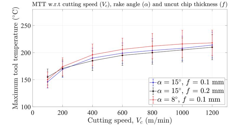
ETNA
Kent State University and
Johann Radon Institute (RICAM)
A COMBINED FINITE ELEMENT AND MACHINE LEARNING APPROACH IN MACHINING 69
F IG . 3.1. Finite element model setup.
strain rate range of 102 to 105 s−1 . The equation is given by
h ¯˙ i h i
(3.1) σ(¯ n ) 1 + C ln
, ¯˙, T ) = (A + B¯ 1 − T̄ m .
˙0
The flow stress is represented as a function of strain ¯, strain rate ¯˙, and the non-dimensional
temperature T̄ . The first term in the equation accounts for isotropic hardening whereas the
second and third terms account for strain rate hardening and thermal softening respectively.
The material parameters A, B, n, C, and m for the JC model are given in Table 3.2 and are
the same as used by [22, 37]. Here, T̄ in (3.1) is given by
0, T < Ttrans ,
T − Ttrans
T̄ = , Ttrans < T < Tmelt ,
T − Ttrans
melt
1, T > Tmelt
where Tmelt is the melting temperature and Ttrans is the transition temperature of the workpiece
material.
TABLE 3.2
Johnson-Cook model parameters for Al 2024-T351.
A B n C m Ttrans Tmelt
(MPa) (MPa) (K) (K)
352 440 0.42 0.0083 1 25 520
3.3. Contact modeling. Contact modeling in the secondary deformation zone, at the
interface of the chip and the rake face of the tool is critical for studying the thermal events at
the chip-tool interface. importance. From experimental results, it has been found and verified
that two contact regions may be distinguished in dry machining: the sticking region, and the
slipping region [24]. Zorev proposed a friction model in [42], where he showed that the normal
stress (σn ) in the secondary deformation zone is maximum at the tool tip and reduces to zero
at a point where the chip loses contact from the rake face. Although Zorev’s model is widely
used to model friction at the tool-chip interface, it has some severe drawbacks. For example,
in the slip zone lslip , the coefficient of friction µ is assumed to be constant and independent of
σn [39].
ETNA
                                                                           Kent State University and
                                                                        Johann Radon Institute (RICAM)

70                   S. MEKARTHY, M. HASHEMITAHERI, AND H. CHERUKURI

     In the present work, to overcome the drawbacks associated with Zorev’s model, the
stress-based friction model proposed by Yang and Liu [40] consisting of both stick and slip
regions was used. For further details on this model, the reader is referred to the work by
Patel et al. [29]. The tool-chip interaction was defined using the penalty stiffness contact
formulation where the tool was considered as master surface and the chip was considered as
slave surface. In addition, the self-contact of the chip was also defined using penalty contact
formulation.
     3.4. Damage modeling. Chip formation takes place as a result of damage and fracture
in a material due to the action of the cutting tool. Finite element simulations require a
criterion to simulate chip separation from the bulk when the tool moves and interacts with
the workpiece. The chip separation criterion should closely reflect the physics and mechanics
of chip formation to achieve reliable results. In this work, the Johnson-Cook damage model
[15] is used to model machining as a process resulting from damage and fracture in a material.
According to this model the overall damage in a material occurs in two steps [1]: damage
initiation and damage evolution.
     Damage initiates in a material when the damage parameter ω defined as:
                                                X ∆¯

(3.2)                                     ω=                ,
                                                      ¯d
equals or exceeds one. The numerator ∆¯    is the increment in equivalent plastic strain, whereas
the denominator ¯d is equivalent plastic strain at the onset of damage initiation and is given by
                    "                         !#"                     !#"          #
                                           p                      ¯˙
              ¯d = D1 + D2 exp D3                 1 + D4 ln              1 + D5 T̄ .
                                           σ̄                    ˙0

The parameters D1 to D5 are shown in the Table 3.3. The parameter D5 is zero which indicates
that temperature does not have any effect on the damage initiation of aluminum [22].

                                            TABLE 3.3
                       Johnson-Cook damage model parameters for Al 2024-T351.

                                D1      D2      D3          D4   D5
                               0.13    0.13     1.5     0.011     0

     The damage evolution is modeled using the damage variable D. It has a value of zero
at the onset of damage and equal to unity when the stiffness of the element is completely
degraded. Two commonly used laws for its evolution are the linear evolution and exponential
evolution. According to linear evolution, the overall damage variable D is defined as:
                                                   ˙ y
                                                  ūσ̄
                                           D=          ,
                                                  2Gf

where ū˙ is the rate of equivalent plastic displacement, Gf the critical energy release rate, and
σ̄y the yield stress after the onset of damage. When D = 1 in an element, the element is
considered to be completely degraded and removed from the model.
     According to exponential evolution, the overall damage variable D is defined as:
                                                 " Z               #
                                                        ū
                                                           σ̄y dū
                                  D = 1 − exp −                      .
                                                      0     Gf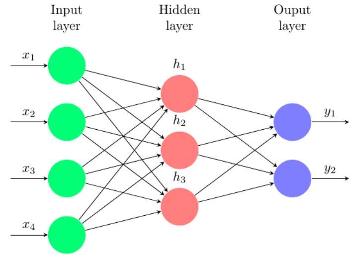
ETNA
Kent State University and
Johann Radon Institute (RICAM)
A COMBINED FINITE ELEMENT AND MACHINE LEARNING APPROACH IN MACHINING 71
Since D approaches one when ū approaches infinity, in Abaqus, D is taken to be one when
the total dissipated energy for each element approaches 0.99 Gf .
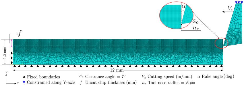
In this work, exponential evolution is defined across the area of uncut chip thickness (f )
whereas linear evolution is defined for the remaining area; see Figure 3.2. This approach and
the values of Gf (critical energy release rate) are adopted from Patel and Cherukuri in [28].
F IG . 3.2. Exponential and linear evolution.
4. Finite element model validation. In this section, the specific cutting forces and chip
morphology obtained from the finite element analysis (FEA) simulations are compared with
the experimental results available in the literature for similar cutting parameters.
The average specific cutting forces obtained from FEA simulations, for rake angle 17.5◦
and uncut chip thicknesses of 0.3 mm and 0.4 mm, during the cutting speeds of 200 m/min,
400 m/min, and 800 m/min are compared with the available experimental results; Asad et
al. [4]. Figures 4.1a and 4.1b show the specific cutting forces and the corresponding difference
respectively.
The difference for the results obtained for uncut chip thickness 0.4 mm is in the range
16% to 19%, whereas for uncut chip thickness 0.3 mm the difference ranges from 15% to 17%.
Moreover, the specific cutting forces remain constant with the increase in cutting speed for
the experimental data. Similar trend is observed for the results obtained from finite element
simulations; see Figure 4.1a.
Chip morphology is a significant parameter to understand the material behavior in ma-
chining. It can be used as a primary parameter in optimizing the metal cutting process since it
reflects the true measure of plastic deformation [6, 20]. The obtained chip morphology is di-
rectly related to the cutting parameters chosen. A high rake angle or a large uncut chip thickness
will result in serrations. Serrations occur due to the instability that arises due to interactions
between strain hardening and thermal softening. Figure 4.2 shows the chip from our simula-
tions for the rake angle 17.5◦ and uncut chip thickness of 0.4 mm with a cutting speed of 800
m/min. This matches closely with the chip obtained in experiments by Mabrouki et al. [22].
5. FEA simulations and data extraction. The data for building ANN models is gener-
ated using the FE model described in Section 3 by varying cutting parameters: the rake angle,
ETNA
                                                                                       Kent State University and
                                                                                    Johann Radon Institute (RICAM)

72                       S. MEKARTHY, M. HASHEMITAHERI, AND H. CHERUKURI

                              (a)                                                  (b)

     F IG . 4.1. Comparison of the specific cutting forces from FEA simulations with the experimental results (4.1a)
and the corresponding difference (4.1b).

      F IG . 4.2. Chip shape predicted by the finite element simulations the rake angle 17.5◦ and uncut chip thickness
of 0.4 mm with a cutting speed of 800 m/min.

uncut chip thickness, and cutting speeds. Simulations are performed for seven rake angles,
four uncut chip thickness values and seven cutting speeds, see Table 5.1, resulting in a total
of 196 (7 × 4 × 7) simulations. The tool nose radius and clearance angle are kept constant
for all the simulations. The total run time for all the simulations is approximately 2350 hours
with each of the FE simulations taking 12 hours on average on Linux-based workstations with
Intel-i7 CPU (3.6 GHz clock rate) and a minimum of 32 GB of RAM. The required output
parameters (specific cutting force and maximum tool temperature) are obtained for all 196
simulations using a Python script.
     6. Artificial neural networks. An artificial neural network structure consists of three
main parts: the input, output, and hidden layers as shown in the Figure 6.1. The first (left)
layer is the input layer and the last (right) layer is the output layer. The layer in between is
hidden layer. Each of these layers has components called neurons; the ones shown as a circle
in Figure 6.1. In a feed-forward neural network, also known as multilayer perceptron (MLP),
the neurons in one layer are connected to the neurons in the next layer and the information
flows forward from the input to the output through the hidden layers. The connections between
the neurons are called synapses. Connections only exist between the neurons of two adjacent
layers but not in the same layer.
     A deep neural network (DNN) has more than one hidden layer (see Figure 7.2) whereas a
shallow neural network (SNN) has only one hidden layer; see Figure 7.1. While deep neural
ETNA
Kent State University and
Johann Radon Institute (RICAM)
A COMBINED FINITE ELEMENT AND MACHINE LEARNING APPROACH IN MACHINING 73
TABLE 5.1
Parameters for simulations.
Rake angle Uncut chip thickness Cutting speed
(deg) (mm) (m/min)
-3 0.1 100
0 0.2 200
5 0.3 400
8 0.4 600
15 800
17.5 1000
20 1200
F IG . 6.1. An example of an artificial neural network (ANN).
networks usually outperform shallow networks on large datasets, for small datasets, shallow
networks may perform just as well or even outperform deep networks in some cases [17, 21, 33].
Neurons consist of a set of input values xi , i = 1, . . . , n, a set of weights wi , i = 1, . . . , n, and
an activation function,Pf ; see Figure 6.3. A linear transformation consisting of the weighted
sum of all the inputs, wi xi , and a bias b is calculated as:
n
X
(6.1) z =b+ w i xi ,
i=1
for each neuron [9]. The output h is calculated from this neuron through the (usually) nonlinear
activation function f (z). Each neuron in a given layer has the same activation function and for
each neuron i in that layer, the output is calculated as hi = f (zi ), where zi is calculated using
(6.1). The outputs serve as the inputs for each of the neurons in the next layer, which can use
a different or the same activation function. The activation function transforms the received
value into a real output through an algorithm. This process is continued until the output layer
is reached where the neurons compute the output variables yi = 1, . . . , k with k as the number
of the outputs.
The activation functions are generally non-linear. Using non-linear activation functions
allows ANN to be applied for complex problems. Few activation functions that are available
in the software packages are sigmoid (logistic function), hyperbolic tangent sigmoid, softmax,
ELU, ReLU, leaky ReLU, linear, etc. Some of the popular activation functions are illustratedETNA
Kent State University and
Johann Radon Institute (RICAM)
74 S. MEKARTHY, M. HASHEMITAHERI, AND H. CHERUKURI
in Figure 6.2. There are no standard methods available in the literature for the number of
hidden layers, neurons, and the activation function. Hence, researchers follow a trial and error
approach.
F IG . 6.2. Some of the popular activation functions. The activation functions are usually enable the neural
networks to consider non-linearity in the data.
F IG . 6.3. A single neuron consists of the inputs xi , the weights wi , and the activation function f (z), which
produces the scalar value h. Note that z is defined with the bias b absorbed into the summation by setting x0 = 1
and w0 = b [8].ETNA
Kent State University and
Johann Radon Institute (RICAM)
A COMBINED FINITE ELEMENT AND MACHINE LEARNING APPROACH IN MACHINING 75
In supervised learning, the training data (input data and the corresponding output data) is
used to train the model. The training starts with an initial assumption on the weights wi . The
input data is processed by the ANN and output is predicted. The error between the predicted
outputs and known outputs is calculated using a cost (or loss) function which can be the sum
of the squares of the errors between predicted and observed outputs, for example. Since the
predicted values depend on the weights and biases, it is clear that the loss function E is also
a function of the weights and biases for a given set of training data, i.e., E = E(wi , b). By
absorbing the bias b into the weights as an additional parameter, E can be assumed to be a
function of only the weights wi . If the error is not acceptable, the weights are updated through
various methods. One approach is the gradient descent method, where the weight updates are
computed using the derivatives of the error function with respect to the weights:
(j)
(j+1) (j) ∂E
(6.2) wi = wi −η .
∂wi
In (6.2) η is the learning rate which is used to control the magnitudes of the corrections
applied to wi . The subscript j indicates the jth iteration. If the value of η is too large, the
model is prone to convergence issues and at the same time if the value is extremely small the
computational time and cost increases. The updated weights are again used for predictions
and calculating the error in predictions. The process is repeated until the error is less than
a pre-selected value or a maximum number of iterations has been reached. Although (6.2)
captures the essence of weight updates, in a typical ANN with multiple hidden layers, the
gradient calculation is quite complicated and involved. Hence, in this work, an Adaptive
moment estimation (Adam) training algorithm was used for updating the weights. Adam
is an algorithm for first-order gradient-based optimization of stochastic objective functions,
based on adaptive estimates of lower-order moments. Adam computes individual adaptive
learning rates for different parameters from the estimates of first and second moments of the
gradients. The algorithm is straight forward to implement and has little memory requirements.
For further details on this training algorithm, the reader is referred to [18].
7. ANN modeling and analysis. Python programming language was used to build the
ANN model. A high-level neural network API (Application programming interface) Keras
was used as the main library. Additional libraries like Pandas, NumPy, and Scikit-learn were
used for data preparation and analysis. In this work, both SNNs and DNNs were built, where
the desired outputs, specific cutting force Ks and maximum tool temperature (MTT) were
predicted individually, i.e., the output layer contains only one neuron; either Ks or MTT. The
input layer has has three input parameters; rake angle α, uncut chip thickness f , and cutting
speed Vc .
The data sets for training and testing were obtained from FE simulations. Table 7.1 shows
the 196 data sets obtained from FEA simulations. The data sets (inputs and outputs) were
normalized to the range [0, 1] using
V − Vmin
(7.1) VN = .
Vmax − Vmin
Here, V denotes the actual values (which are to be normalized) Vmin , Vmax denote the minimum
and maximum values. Normalizing the data sets is essential to ensure the data sets to be
present in a logical correlation. If they are not normalized, the network could possibly consider
the data set with higher arithmetic value to be more significant than others. This may affect
the generalization ability of the network and can also lead to over fitting [25].ETNA
Kent State University and
Johann Radon Institute (RICAM)
76 S. MEKARTHY, M. HASHEMITAHERI, AND H. CHERUKURI
The normalized data was split into training and testing sets using an 80:20 ratio. A further
10% of validation split was performed on the training data set. This was determined to be the
most reasonable split after trying different proportions. Thus, the training set consisted of 140
data points, while the validation and test sets consisted of 16 and 40, respectively. During the
prediction of specific cutting forces, the maximum tool temperature column from Table 7.1
was excluded, and during the prediction of maximum tool temperature, the cutting force data
was excluded.
TABLE 7.1
Data obtained from finite element simulations.
Input parameters Outputs
S.No. Rake angle Uncut chip thickness Cutting speed Specific cutting force Maximum tool temperature
(deg◦ ) (mm) (m/min) (N/mm2 ) (K)
1 -3 0.1 100 874 164
2 -3 0.1 200 895 184
3 -3 0.1 400 945 208
. . . . . .
. . . . . .
. . . . . .
48 0 0.3 1000 667 246
49 0 0.3 1200 678 249
50 0 0.4 100 681 188
. . . . . .
. . . . . .
84 5 0.4 1200 599 259
85 8 0.1 100 758 150
. . . . . .
. . . . . .
. . . . . .
140 15 0.4 1200 506 229
141 17.5 0.1 100 678 144
. . . . . .
. . . . . .
. . . . . .
. . . . . .
195 20 0.4 1000 453 226
196 20 0.4 1200 495 232
Figure 7.1 shows the SNN built in this work for predicting Ks . We also used the same
architecture to predict MTT. During the SNN training, the number of neurons in the hidden
layer was varied from five to twenty five and five activation functions (ReLU, ELU, tanh,
sigmoid and linear) were employed resulting in 105 SSN architectures for each Ks and MTT.
Figure 7.2 shows the DNN built to predict Ks . We used the same network architecture to
predict MTT. In both the cases neurons in the first two hidden layers were varied from five to
fifteen, whereas the neurons in the third hidden layer were varied from zero to three. The same
five activation functions, mentioned above, were used during the training. A total of 800 DNN
architectures were built for predicting each Ks and MTT. The number of epochs and batch
size were determined to be 150 and 20, respectively, by a trial and error approach. Epochs
define how many times the model will be trained through the entire training data set. Batch
size determines the number of training samples sent together to the network. For instance,
having 1000 data records, setting 10 epochs and batch size of 20 means the network will iterate
the training data 10 times. In each iteration, 50 batches are sent to the network and in each
batch, the model is trained on 20 data records simultaneously.ETNA
Kent State University and
Johann Radon Institute (RICAM)
A COMBINED FINITE ELEMENT AND MACHINE LEARNING APPROACH IN MACHINING 77
Hidden layer
Input layer Output layer
Rake angle (deg◦)
Uncut chip thickness (mm) Specific cutting force (N/mm2)
Cutting speed (m/min)
F IG . 7.1. SNN for predicting Ks .
Input layer Hidden layers Output layer
Rake angle (deg◦)
Uncut chip thickness (mm) Specific cutting force (N/mm2)
Cutting speed (m/min)
F IG . 7.2. DNN for predicting Ks .
One important point to be noted is that, linear activation function was used as the default
between the output layer and the hidden layer preceding it for all the network architectures.
As soon as the training process was completed, the test data sets were fed to the trained neural
networks to determine the architecture that exhibited the least error in prediction. For this
purpose, statistical evaluations were performed using the mean squared error (MSE)
n
1X
(7.2) MSE = (yi − yip )2
n i=1
and coefficient of determination R2 using
n
(yi − yip )2
P
(7.3) R2 = 1 − i=1
Pn .
(yi − ȳ)2
i=1
In (7.2) and (7.3), yi represents the actual output, yip represents the ANN predicted output,
and ȳ represents the mean of the actual outputs. The network architecture with the highest R2
and least MSE on the test data set is concluded to be the suitable network [36].ETNA
Kent State University and
Johann Radon Institute (RICAM)
78 S. MEKARTHY, M. HASHEMITAHERI, AND H. CHERUKURI
8. Predictions from ANN models. In this section, the results from the two ANN models
for the prediction of maximum tool temperature and specific cutting force are presented.
8.1. Prediction of maximum tool temperature. Among the 905 ANN models (SNN +
DNN) that were built, the model with the network architecture 3-15-14-3-1 with the activation
function ReLU has the highest R2 (0.9605) and least MSE (0.00227) on the test data. Figure
8.1 shows the predictions made by this network. It is observed that, the predictions are in
close agreement with actual outputs. After examining the predictions, it can be stated that
the network architecture 3-15-14-3-1 is the suitable network for predicting the maximum
temperature on the cutting tool.
260
240
220
200
180
160
140
140 160 180 200 220 240 260
F IG . 8.1. Relation between actual values and ANN predicted values for maximum tool temperature.
TABLE 8.1
Top 10 DNNs and top SNN for predicting maximum tool temperature.
Training Testing
S No Activation function Network type Network architecture Hidden layers MSE R2 MSE R2
1 ReLU DNN 3-15-14-3-1 3 0.00113 0.9747 0.00227 0.9605
2 ReLU DNN 3-14-13-3-1 3 0.00113 0.9748 0.00228 0.9603
3 ReLU DNN 3-12-13-3-1 3 0.00124 0.9721 0.00235 0.9593
4 ReLU DNN 3-11-12-3-1 3 0.00144 0.9677 0.00237 0.9588
5 ReLU DNN 3-11-10-3-1 3 0.00151 0.9662 0.00238 0.9587
6 ReLU DNN 3-13-13-3-1 3 0.00147 0.9671 0.00248 0.9570
7 ReLU DNN 3-13-12-0-1 2 0.00140 0.9687 0.00249 0.9568
8 ReLU DNN 3-15-15-0-1 2 0.00177 0.9603 0.00250 0.9566
9 ReLU DNN 3-14-14-3-1 3 0.00146 0.9674 0.00256 0.9555
10 ReLU DNN 3-11-12-0-1 2 0.00166 0.9628 0.00265 0.9540
ReLU SNN 3-23-0-0-1 1 0.00187 0.9582 0.00301 0.9477
Table 8.1 presents the performance of the top 10 deep neural network architectures and
top shallow network arranged in increasing order of MSE (or decreasing order of R2 ) with
respect to the test data set. It is interesting to note that neural networks with ReLU as the
activation function have performed well compared to other activation functions.ETNA
Kent State University and
Johann Radon Institute (RICAM)
A COMBINED FINITE ELEMENT AND MACHINE LEARNING APPROACH IN MACHINING 79
8.2. Prediction of specific cutting force. Among the 905 ANN models (SNN+DNN),
the neural network model with the architecture 3-9-10-0-1 (0 indicates that there are no neurons
in the third hidden layer.) with ReLU as the activation function has the highest R2 (0.9419)
and least MSE (0.0022) with respect to the test data. After examining the plot (Figure 8.2)
which shows the predictions made by this neural network, it can be stated that the network
architecture 3-9-10-0-1 predicts outputs closest to the actual outputs.
900
800
700
600
500
500 600 700 800 900
F IG . 8.2. Relation between actual values and ANN predicted values for specific cutting force.
TABLE 8.2
Top 10 DNNs and top SNN for predicting specific cutting force.
Training Testing
S. No Activation function Network type Network architecture Hidden layers MSE R2 MSE R2
1 ReLU DNN 3-9-10-0-1 2 0.00294 0.9394 0.00220 0.9419
2 ReLU DNN 3-8-9-0-1 2 0.00261 0.9463 0.00230 0.9395
3 ELU DNN 3-13-13-3-1 3 0.00290 0.9403 0.00243 0.9359
4 ReLU DNN 3-14-15-3-1 3 0.00247 0.9492 0.00246 0.9352
5 ReLU DNN 3-15-15-0-1 2 0.00242 0.9502 0.00248 0.9348
6 ReLU DNN 3-13-13-0-1 2 0.00282 0.9420 0.00248 0.9347
7 tanh DNN 3-15-14-3-1 3 0.00310 0.9361 0.00253 0.9335
8 tanh DNN 3-13-12-3-1 3 0.00304 0.9375 0.00255 0.9329
9 ReLU DNN 3-5-5-0-1 2 0.00322 0.9338 0.00258 0.9322
10 ELU DNN 3-6-5-0-1 2 0.00310 0.9362 0.00259 0.9320
ReLU SNN 3-18-0-0-1 1 0.00337 0.9305 0.00291 0.9235
Table 8.2 presents the performance of the top 10 deep neural network architectures and
top shallow network arranged in increasing order of MSE (or decreasing order of R2 ) with
respect to the test data set. It is observed that the neural network with ReLU as the activation
function has the best performance, which is similar to the results of maximum tool temperature
model.
8.3. Experimental verification. The network architecture 3-9-10-0-1 which was se-
lected for specific cutting force prediction, was further evaluated with the available experimen-ETNA
Kent State University and
Johann Radon Institute (RICAM)
80 S. MEKARTHY, M. HASHEMITAHERI, AND H. CHERUKURI
tal data. That is, the experimental data sets available in the literature [4, 7, 19, 23] were given
as the inputs to this neural network and the corresponding outputs (Ks ) were predicted and
the difference was calculated.
Figure 8.3 shows the actual experimental outputs and the outputs predicted by this neural
network. With the exception of a couple of outliers, the predicted values are clearly in good
agreement with the experimental values. The corresponding difference in prediction is shown
in Figure 8.4. The negative difference for certain data sets indicate that the neural network has
over-predicted the experimental output.
1200
1100
1000
900
800
700
600
600 800 1000 1200
F IG . 8.3. ANN predicted outputs and actual experimental outputs.
10
5
0
-5
-10
0 5 10 15 20
F IG . 8.4. Difference (%) between experimental output and ANN predicted output.ETNA
Kent State University and
Johann Radon Institute (RICAM)
A COMBINED FINITE ELEMENT AND MACHINE LEARNING APPROACH IN MACHINING 81
9. Sensitivity analysis. Sensitivity studies are extremely important for network designers
to predict the effect of input perturbations on the network’s output [41]. Sensitivity analysis
results tell how likely the outputs based upon the selected model will change on giving new
information. The sensitivity of each input is represented by a numerical value, called the
sensitivity index.
Sensitivity analysis is carried out by using the open source library SALib [12] available
for Python language. This library is capable of generating the model inputs and computing the
sensitivity indices from the model outputs. We used the Sobol method [31, 32, 34] available
in SALib Package for the purpose of this analysis.
Sobol’s method analyzes the portion of variance in the output of the network that is
explained by each input variable or each subset of the input variables. Sensitivity indices are
available in several forms. We focus on the first-order indices measuring only the effect of a
single input variable [12]. First, we provide a brief sketch of the method.
Let X = (x1 , . . . , xn ) denote the input variables of the network and without loss of
generality, assume xi ∈ [0, 1]. Furthermore, let Y = φ(X) denote the network output. We
may write Y as the sum of simpler orthogonal functions:
n
X n
X
(9.1) Y = φ(X) = φ0 + φi (xi ) + φij (xi , xj ) + · · · + φ12...n (x1 , x2 , . . . , xn )
i=1 iETNA
Kent State University and
Johann Radon Institute (RICAM)
82 S. MEKARTHY, M. HASHEMITAHERI, AND H. CHERUKURI
Comparing with (9.5), we can immediately observe that the sum of all sensitivity indices
is equal to one:
n
X X
(9.7) ψjr ...jt = 1
t=1 jrETNA
Kent State University and
Johann Radon Institute (RICAM)
A COMBINED FINITE ELEMENT AND MACHINE LEARNING APPROACH IN MACHINING 83
F IG . 9.1. Specific cutting forces obtained from FEA simulations.
F IG . 9.2. Maximum tool temperatures obtained from FEA simulations.
10. Conclusions. The paper presented a comprehensive analysis of the application of
FEM and ANN to predict specific cutting forces and maximum tool temperatures, including
a detailed description of modeling orthogonal machining. A total of 196 simulations were
performed for various rake angles, uncut chip thickness, and cutting speeds for generating
data. In this study, 905 neural network models were built for each specific cutting force and
maximum tool temperature prediction. The suitable neural network architecture for predicting
specific cutting forces is found to be 3-9-10-0-1, with ReLU as the activation function, whereas
for predicting maximum tool temperatures the neural network architecture 3-15-14-3-1, with
ReLU as the activation function, was found to be suitable. Sensitivity analysis was performed
to check the sensitivity of the output with input perturbations, and results revealed that, specific
cutting forces are sensitive to both rake angle and uncut chip thickness. On the other hand,
maximum tool temperatures were found to be sensitive to cutting speeds.ETNA
Kent State University and
Johann Radon Institute (RICAM)
84 S. MEKARTHY, M. HASHEMITAHERI, AND H. CHERUKURI
The work reveals that the hybrid approach of combining FEM and machine learning to
predict specific cutting forces and maximum tool temperatures is effective. The coefficient
of determination R2 can be improved by adding more number of data sets during the ANN
modeling process.
The proposed approach can be extended for other work materials and manufacturing
applications. Additional parameters like stresses, strains, and tool-tip temperatures can be
predicted. More advanced training algorithms, such as Nadam and Adamax, can be used
along with the application of other activation functions, including leaky ReLU, PReLU, and
Thresholded ReLU.
11. Acknowledgements. The Center for Self-Aware Manufacturing and Metrology, and
the research described in this paper, are supported under a multi-year grant from the University
of North Carolina’s Research Opportunities Initiative. The first author wishes to thank Nishant
Ojal for helping making the neural network figures in this paper.
REFERENCES
[1] Abaqus 2017 documentation. http://130.149.89.49:2080/v2016/index.html.
[2] A. H. A DIBI -S EDEH , V. M ADHAVAN , AND B. BAHR, Extension of Oxley’s analysis of machining to use
different material models, J. Manuf. Sci. Eng., 125 (2003), pp. 656–666.
[3] A. A L -A HMARI, Predictive machinability models for a selected hard material in turning operations,
J. Mater. Process. Technol., 190 (2007), pp. 305–311.
[4] M. A SAD , F. G IRARDIN , T. M ABROUKI , AND J.-F. R IGAL, Dry cutting study of an aluminium alloy
(A2024-T351): a numerical and experimental approach, Int. J. Mater. Form., 1 (2008), pp. 499–502.
[5] P. A SOKAN , R. R. K UMAR , R. J EYAPAUL , AND M. S ANTHI, Development of multi-objective optimization
models for electrochemical machining process, Int. J. Adv. Manuf. Technol., 39 (2008), pp. 55–63.
[6] V. P. A STAKHOV AND S. S HVETS, The assessment of plastic deformation in metal cutting, J. Mater. Pro-
cess. Technol., 146 (2004), pp. 193–202.
[7] S. ATLATI , B. H ADDAG , M. N OUARI , AND M. Z ENASNI, Analysis of a new segmentation intensity ratio “SIR”
to characterize the chip segmentation process in machining ductile metals, Int. J. Mach. Tools Manuf., 51
(2011), pp. 687–700.
[8] H. C HERUKURI , E. P EREZ -B ERNABEU , M. S ELLES , AND T. L. S CHMITZ, A neural network approach for
chatter prediction in turning, Procedia Manuf., 34 (2019), pp. 885–892.
[9] H. C HERUKURI , E. P EREZ -B ERNABEU , M. A. S ELLES , AND T. S CHMITZ, Machining chatter prediction
using a data learning model, J. Manuf. Mater. Process., 3 (2019).
[10] M. C ORREA , C. B IELZA , AND J. PAMIES -T EIXEIRA, Comparison of Bayesian networks and artificial neural
networks for quality detection in a machining process, Expert Syst. Appl., 36 (2009), pp. 7270–7279.
[11] S. S. H AYKIN, Neural Networks and Learning Machines, 3rd. ed., Pearson, Upper Saddle River, 2009.
[12] J. H ERMAN AND W. U SHER, SALib: An open-source Python library for sensitivity analysis,
J. Open Source Softw., 2 (2017), doi:10.21105/joss.00097.
[13] Y. H UANG AND S. L IANG, Cutting forces modeling considering the effect of tool thermal property–application
to CBN hard turning, Int. J. Mach. Tools Manuf., 43 (2003), pp. 307–315.
[14] G. J OHNSON AND W. C OOK, A constitutive model and data for metals subjected to large strains, strain rates,
and high pressures, in Proceedings of the 7th International Symposium On Ballistics, The Hague, 1983,
pp. 541–548.
[15] G. R. J OHNSON AND W. H. C OOK, Fracture characteristics of three metals subjected to various strains,
strain rates, temperatures and pressures, Eng. Fract. Mech., 21 (1985), pp. 31–48.
[16] F. K ARA , K. A SLANTAS , AND A. Ç IÇEK, ANN and multiple regression method-based modelling of cutting
forces in orthogonal machining of AISI 316L stainless steel, Neural Comput. Appl., 26 (2015), pp. 237–
250.
[17] D. E. K IM AND M. G OFMAN, Comparison of shallow and deep neural networks for network intrusion
detection, in 2018 IEEE 8th Annual Computing and Communication Workshop and Conference (CCWC),
IEEE Conference Proceedings, Los Alamitos, 2018, pp. 204–208.
[18] D. P. K INGMA AND J. BA, Adam: A method for stochastic optimization, arXiv Preprint, arXiv:1412.6980,
2014. https://arxiv.org/abs/1412.6980.
[19] S. KOBAYASHI , R. H ERZOG , D. E GGLESTON , AND E. T HOMSEN, A critical comparison of metal-cutting
theories with new experimental data, J. Eng. Ind., 82 (1960), pp. 333–347.
[20] S. KOUADRI , K. N ECIB , S. ATLATI , B. H ADDAG , AND M. N OUARI, Quantification of the chip segmentationETNA
Kent State University and
Johann Radon Institute (RICAM)
A COMBINED FINITE ELEMENT AND MACHINE LEARNING APPROACH IN MACHINING 85
in metal machining: Application to machining the aeronautical aluminium alloy AA2024-T351 with
cemented carbide tools WC-Co, Int. J. Mach. Tools Manuf., 64 (2013), pp. 102–113.
[21] S. L IANG AND R. S RIKANT, Why deep neural networks for function approximation?, arXiv Preprint,
arXiv:1610.04161, 2016. https://arxiv.org/abs/1610.04161.
[22] T. M ABROUKI , F. G IRARDIN , M. A SAD , AND J.-F. R IGAL, Numerical and experimental study of dry cutting
for an aeronautic aluminium alloy (A2024-T351), Int. J. Mach. Tools Manuf., 48 (2008), pp. 1187–1197.
[23] M. M ADAJ AND M. P ÍŠKA, On the SPH orthogonal cutting simulation of A2024-T351 alloy, Procedia CIRP,
8 (2013), pp. 152–157.
[24] A. P. M ARKOPOULOS, Finite Element Method in Machining Processes, Springer, London, 2012.
[25] A. P. M ARKOPOULOS , D. E. M ANOLAKOS , AND N. M. VAXEVANIDIS, Artificial neural network models
for the prediction of surface roughness in electrical discharge machining, J. Intell. Manuf., 19 (2008),
pp. 283–292.
[26] İ. OVALI AND A. M AVI, A study on cutting forces of austempered gray iron using artificial neural networks,
Eng. Sci. Technol. an Int., 16 (2013) pp. 1–10.
[27] T. Ö ZEL AND E. Z EREN, A methodology to determine work material flow stress and tool-chip interfacial
friction properties by using analysis of machining, J. Manuf. Sci. Eng., 128 (2006), pp. 119–129.
[28] J. PATEL AND H. P. C HERUKURI, Chip morphology studies using separate fracture toughness values for
chip separation and serration in orthogonal machining simulations, in ASME 2018 13th International
Manufacturing Science and Engineering Conference, American Society of Mechanical Engineers, New
York, 2018, V002T04A031.
[29] J. P. PATEL, Finite Element Studies of Orthogonal Machining of Aluminum Alloy A2024-T351, PhD. Thesis,
The University of North Carolina, Charlotte, 2018.
[30] F. J. P ONTES , J. R. F ERREIRA , M. B. S ILVA , A. P. PAIVA , AND P. P. BALESTRASSI, Artificial neural
networks for machining processes surface roughness modeling, Int. J. Adv. Manuf. Technol., 49 (2010),
pp. 879–902.
[31] A. S ALTELLI, Making best use of model evaluations to compute sensitivity indices, Comput. Phys. Commun.,
145 (2002), pp. 280–297.
[32] A. S ALTELLI , P. A NNONI , I. A ZZINI , F. C AMPOLONGO , M. R ATTO , AND S. TARANTOLA, Variance
based sensitivity analysis of model output. design and estimator for the total sensitivity index, Com-
put. Phys. Commun., 181 (2010), pp. 259–270.
[33] A. S CHINDLER , T. L IDY, AND A. R AUBER, Comparing shallow versus deep neural network architectures for
automatic music genre classification, in Proceedings of the 9th Forum Media Technology (FMT2016),
W. Aigner, G. Schmiedl, K. Blumenstein, eds., Lulu.com, Morrisville, 2016, pp. 17–21.
[34] I. M. S OBOL, Global sensitivity indices for nonlinear mathematical models and their Monte Carlo estimates,
Math. Comput. Simulation, 55 (2001), pp. 271–280.
[35] S. TASDEMIR, Artificial neural network based on predictive model and analysis for main cutting force in
turning, Energy Education Science and Technology Part A-Energy Science and Research, 29 (2012),
pp. 1471–1480.
[36] S. TASDEMIR, Artificial neural network model for prediction of tool tip temperature and analysis, Int. J. In-
tell. Syst. Appl. Eng, 6 (2018), pp. 92–96.
[37] X. T ENG AND T. W IERZBICKI, Evaluation of six fracture models in high velocity perforation,
Eng. Fract. Mech., 73 (2006), pp. 1653–1678.
[38] A. E. T UMER AND S. E DEBALI, An artificial neural network model for wastewater treatment plant of Konya,
Int. J. Intell. Syst. Appl. Eng., 3 (2015), pp. 131–135.
[39] P. WALLACE AND G. B OOTHROYD, Tool forces and tool-chip friction in orthogonal machining,
J. Mech. Eng. Sci., 6 (1964), pp. 74–87.
[40] X. YANG AND C. R. L IU, A new stress-based model of friction behavior in machining and its significant
impact on residual stresses computed by finite element method, Int. J. Mech. Sci., 44 (2002), pp. 703–723.
[41] X. Z ENG AND D. S. Y EUNG, Sensitivity analysis of multilayer perceptron to input and weight perturbations,
IEEE Trans. Neural Netw., 12 (2001), pp. 1358–1366.
[42] N. Z OREV, Inter-relationship between shear processes occurring along tool face and shear plane in metal
cutting, Int. Res. Prod. Eng., 49 (1963), pp. 143–152.You can also read