Ventilation and Transformation of Labrador Sea Water and Its Rapid Export in the Deep Labrador Current
←
→
Page content transcription
If your browser does not render page correctly, please read the page content below
946                              JOURNAL OF PHYSICAL OCEANOGRAPHY                                                             VOLUME 37

  Ventilation and Transformation of Labrador Sea Water and Its Rapid Export in the
                               Deep Labrador Current
        PETER BRANDT, ANDREAS FUNK, LARS CZESCHEL, CARSTEN EDEN,                                AND    CLAUS W. BÖNING
                            IFM-GEOMAR, Leibniz-Institut für Meereswissenschaften, Kiel, Germany

                                   (Manuscript received 1 June 2005, in final form 31 July 2006)

                                                            ABSTRACT

               A model of the subpolar North Atlantic Ocean is used to study different aspects of ventilation and water
            mass transformation during a year with moderate convection intensity in the Labrador Sea. The model
            realistically describes the salient features of the observed hydrographic structure and current system,
            including boundary currents and recirculations. Ventilation and transformation rates are defined and com-
            pared. The transformation rate of Labrador Sea Water (LSW), defined in analogy to several observational
            studies, is 6.3 Sv (Sv ⬅ 106 m3 s⫺1) in the model. Using an idealized ventilation tracer, mimicking analyses
            based on chlorofluorocarbon inventories, an LSW ventilation rate of 10 Sv is found. Differences between
            both rates are particularly significant for those water masses that are partially transformed into denser water
            masses during winter. The main export route of the ventilated LSW is the deep Labrador Current (LC).
            Backward calculation of particle trajectories demonstrates that about one-half of the LSW leaving the
            Labrador Sea within the deep LC originates in the mixed layer during that same year. Near the offshore
            flank of the deep LC at about 55°W, the transformation of LSW begins in January and is at a maximum in
            February/March. While the export of transformed LSW out of the central Labrador Sea continues for
            several months, LSW generated near the boundary current is exported more rapidly, with maximum
            transport rates during March/April within the deep LC.

1. Introduction                                                      depths, is composed of the West Greenland Current
                                                                     (WGC), the Irminger Current (IC), the Labrador Cur-
   The Atlantic Ocean meridional overturning circula-                rent (LC), and the North Atlantic Current (NAC) with
tion (MOC), composed of a northward warm water                       its “Northwest Corner.” The WGC imports fresh and
flow in the near-surface layer and a southward flow of               cold water near the surface at the shelf, and the IC
North Atlantic Deep Water (NADW), represents an                      transports warmer and saltier water at intermediate
important part of the global climate system due to its               depths into the Labrador Sea (Lazier et al. 2002).
associated northward heat transport. Besides the over-               Downstream of this inflow region, the initially strong
flow regions between Greenland and Iceland, as well as
                                                                     temperature maximum at intermediate depths de-
between Iceland and Scotland, open ocean convection
                                                                     creases. At the shelf off Labrador at about 53°N, the
in the Labrador Sea contributes considerably to the
                                                                     southeastward deep LC is found to transport about 26
generation of NADW. In this region, strong oceanic
                                                                     Sv (Sv ⬅ 106 m3 s⫺1) of NADW, of which about 11 Sv
heat loss in winter leads to the transformation of upper
                                                                     are transported within the potential density range of
NADW, the so-called Labrador Sea Water (LSW),
                                                                     LSW. The deep LC has a strong barotropic component
overlying the deep waters from the overflow regions
                                                                     and extends approximately out to the 3300-m depth
(Marshall and Schott 1999). The cyclonic circulation in
                                                                     contour (Fischer et al. 2004). Offshore of the deep LC,
the Labrador Sea, a necessary condition for deep con-
                                                                     several cyclonic recirculation cells exist that are associ-
vection associated with large late winter mixed layer
                                                                     ated with an interior anticyclonic circulation around the
                                                                     central Labrador Sea as well as a doming of the isopy-
                                                                     cnals off the boundary current (Lavender et al. 2000).
  Corresponding author address: Peter Brandt, IFM-GEOMAR,
Leibniz-Institut für Meereswissenschaften, Düsternbrooker Weg        While there are different export routes of LSW out of
20, 24105 Kiel, Germany.                                             the Labrador Sea, that is, into the Irminger Sea and to
E-mail: pbrandt@ifm-geomar.de                                        the east—even crossing the Mid-Atlantic Ridge (Sy et

DOI: 10.1175/JPO3044.1

© 2007 American Meteorological Society

 JPO3044
APRIL 2007                                      BRANDT ET AL.                                                      947

al. 1997; Fischer and Schott 2002; Rhein et al. 2002)—       results obtained using different measurement tech-
the direct route along the Deep Western Boundary             niques.
Current appears to represent the fastest communica-             Here, we want to address the following questions
tion between the subpolar convection region and the          that are hard to assess from observational results: How
subtropical gyre (Schott et al. 2004).                       much LSW exiting the Labrador Sea was within the
   The maximum late winter mixed layer depths in the         mixed layer in the same year? Where and when does
Labrador Sea are observed offshore of the deep LC            the water mass transformation take place, and where
(Lavender et al. 2000). In this region, classical or deep    and when does the LSW leave the mixed layer? After
LSW is generated during years of medium to deep con-         describing the model, which we use to answer these
vection. In addition to the classical LSW, Pickart et al.    questions, the methods to analyze its output fields, and
(1997, 2002) suggested that the transformation of upper      the general characteristics of the model solution in sec-
LSW occurs in the western boundary current region.           tion 2, the pathways of ventilated water including its
However, the strength of Labrador Sea convection var-        subduction are analyzed by introducing an idealized
ies strongly from year to year with deep convection in       ventilation tracer and by calculating backward Lagran-
the early 1990s followed by a multiyear restratification     gian drifter trajectories in section 3. In section 4, the
period (Lazier et al. 2002). For the “post deep convec-      water mass transformation is analyzed by calculating
tion” period, 1996–2001, Stramma et al. (2004) as well       the local volume change and horizontal divergence, and
as Kieke et al. (2006) suggested a predominant trans-        by evaluating the effect of surface buoyancy fluxes. Dis-
formation of upper LSW that increasingly filled the up-      cussion and conclusions are presented in section 5.
per levels of the central Labrador Sea.
   Here, we study some basic aspects of the transforma-
tion of LSW and its export out of the Labrador Sea           2. Numerical model, methods, and general
using an eddy-resolving numerical model of the subpo-           characteristics
lar North Atlantic. Besides identifying transformation
                                                             a. Model
regions and exit pathways, we want to address the re-
lation between ventilation and transformation of LSW.           We discuss results of a regional eddy-resolving model
While transformation is defined here as the total LSW        developed as part of the Family of Linked Atlantic
volume change due to diapycnal fluxes, ventilation—          Ocean Model Experiments (FLAME). The model
which is associated with air–sea fluxes of trace gases—      domain covers the subpolar North Atlantic from 43°
occurs when LSW is part of the mixed layer and thus in       to 70°N, 71°W to 16°E. The model code is a rewrit-
contact with the atmosphere. In general, ventilation         ten version of the Modular Ocean Model version
rates and transformation rates may differ for a given        2 (MOM2) Code (Pacanowski 1995) and can be
potential density range.                                     found online (http://www.ifm-geomar.de/index.
   Transformation rates, which are a controlling factor      php?id⫽spflame). Primitive equations were solved on
for the Atlantic MOC and meridional heat fluxes, have        an Arakawa-B grid (Arakawa and Lamb 1977) with
been estimated from observations using different             horizontal resolution of 1/12° in longitude, square grid
datasets and/or methods: among them are air–sea              boxes (i.e., about 5 km and thus “eddy resolving” in the
fluxes of heat and freshwater (e.g., Speer and Tziper-       Labrador Sea) and 45 vertical levels with a thickness of
man 1992; Marsh 2000; Khatiwala et al. 2002) and in-         10 m at the surface, increasing to 250 m at the maximum
verse methods (Talley 2003; Pickart and Spall 2007).         depth of 4500 m. The model setup is essentially the
On the other hand, the increase with time of chloroflu-      same as in Eden and Böning (2002) except for the fol-
orocarbon (CFC) inventories within a particular poten-       lowing differences: the domain is reduced to the sub-
tial density range reflects a ventilation of this water by   polar North Atlantic using open boundaries (Stevens
surface contact. Using additional assumptions regard-        1991) at the northern and southern margins of the do-
ing the equilibrium concentration with the atmosphere        main; harmonic diffusion and friction are replaced by
and the degree of CFC saturation of ventilated water,        isopycnal diffusion (using a diffusivity of 50 m2 s⫺1) and
this method has also been proposed for estimating for-       biharmonic friction (using a viscosity of 2 ⫻ 1010
mation rates of LSW (Smethie and Fine 2001; Rhein et         m4 s⫺1); and the bottom boundary layer parameteriza-
al. 2002; Kieke et al. 2006). However, ventilation rates     tion of Beckmann and Döscher (1997) is used.
are essential for the oceanic gas uptake and the global         Model simulations of the subpolar North Atlantic,
CO2 cycle or for estimating the water mass age. Knowl-       including the one in Eden and Böning (2002), tend to
edge of differences between transformation and venti-        be biased in their hydrographic properties; that is, they
lation rates are therefore important when comparing          often show an ongoing salinification of the Labrador
948 JOURNAL OF PHYSICAL OCEANOGRAPHY VOLUME 37
Sea (Treguier et al. 2005). As shown in Czeschel (2004), specifically with respect to the eddy variability in the
the present model shows significantly improved hydro- boundary current regime, we have for comparison also
graphic properties in comparison to previous model ex- analyzed a companion 1-yr run of a basin-scale version
periments. This is a combined effect of (i) using an open of the 1/12° FLAME model that differs only in the open
northern boundary in the Greenland Sea at 70°N, al- southern boundary shifted toward 18°S. All other as-
lowing for a more realistic inflow of freshwater into the pects of both models including spinup period and
subpolar North Atlantic via the East Greenland Cur- northern boundary formulation are the same.
rent and outflow of saline water via the northward ex-
tension of the North Atlantic Current (Czeschel 2004), b. Methods
and (ii) minimizing spurious diapycnal mixing by the
In the following section we describe the methods
isopycnal mixing scheme. Note that previous models,
used to analyze the numerical simulation that permit a
for example, those discussed in Eden and Böning
distinction between ventilation and transformation
(2002) and Treguier et al. (2005), typically used a north-
rates. Here we applied two methods to quantify venti-
ern temperature and salinity relaxation zone instead of
lation rates in the model: 1) an idealized “ventilation
an open boundary formulation. In addition to the
tracer,” similar to CFC, which is initialized in the mixed
northern boundary, there is also a southern open
layer and is subject to advection and diffusion, and 2)
boundary in the model along 43°N, allowing for inflow
Lagrangian drifters, which are seeded at a section
of the North Atlantic Current and outflow of the con-
across the deep LC (the main export route of LSW out
tinuation of the Labrador Sea boundary current. While
of the Labrador Sea) and followed backward in time,
for the northern open boundary the barotropic inflow
eventually traced back to the mixed layer. The trans-
and outflow are prescribed (taken from a regional
formation rate of the model is calculated on a daily
model simulation of the Arctic Ocean; R. Gerdes 2004,
basis as the sum of local volume change and horizontal
personal communication), at the southern boundary
divergence for an isopycnal layer in predefined boxes.
the inflow/outflow is calculated using a simple Orlanski
Additionally, the transformation rate exclusively due to
radiation condition (Orlanski 1976; as is the baroclinic
negative surface buoyancy flux is calculated. The sec-
inflow/outflow in both cases). For inflow situations,
ond method is applied to each horizontal grid cell,
temperature and salinity values are taken from a com-
thereby yielding additional detailed regional distribu-
bined climatology of Levitus and Boyer (1994) and
tion of this transformation rate.
Boyer and Levitus (1997), which is also used for the
initial condition.
1) VENTILATED LSW
The surface forcing is given by climatological
monthly mean fields taken from a 6-hourly analysis at The first question that we want to address is: How
the European Centre for Medium-Range Weather much of the LSW exiting the Labrador Sea was within
Forecasts (ECMWF) of the years 1986–88 (Barnier et the mixed layer during the same year? In the following,
al. 1995). For the heat flux Q, the following condition is such water will be referred to as newly ventilated or
used: simply as ventilated water. The mixed layer depth is
defined using a potential density () criterion: water
Q ⫽ Q0 ⫹ Q2共SSTmodel ⫺ SSTclim兲, 共1兲
with differences in of less than 0.01 kg m⫺3 from the
where Q0 is the prescribed heat flux, SSTmodel is the surface value is defined as part of the mixed layer.
model sea surface temperature (SST), SSTclim is the SST The time-varying distribution of ventilated water is
corresponding to surface forcing, and Q2 ⫽ Q/SST|SSTclim, investigated using an idealized dimensionless concen-
a function of space and time, is derived from a linear- tration C of a ventilation tracer. The evolution of the
ized form of the bulk formula for surface heat flux tracer concentration is calculated during the model in-
(Barnier et al. 1995). Following usual practice because tegration. The ventilation tracer is initialized with 0 in
of the lack of appropriate data, the freshwater fluxes the entire model domain at 1 January and set to a value
are calculated by restoring sea surface salinities to Levi- of 1 within the mixed layer in the Labrador Sea north of
tus data using a constant time scale of 15 days for the 52°N and west of 43°W (see Fig. 1a) during each time
uppermost 10-m grid boxes. Starting from rest using step beginning at 1 January. The tracer distribution is
Levitus climatology, the model was allowed to spin up calculated for each time step by a tracer equation in-
for 10 model years while forced by the ECMWF clima- cluding advective and diffusive terms identical to the
tology described above. Here we have analyzed a 1-yr terms used in the equations for temperature and salin-
run (model year 10) obtained with the regional model. ity. We define the volume-integrated tracer over the
For testing the robustness of the obtained results, entire model domain,
APRIL 2007 BRANDT ET AL. 949
VC 共t兲 ⫽ 冕 V
C共t兲 dV, 共2兲
as the total volume of water that was ventilated in the
prescribed region (north of 52°N and west of 43°W)
between time t ⫽ 0 (1 January) and the time t.
The ventilation tracer concentration in a certain lo-
cation represents a ratio of ventilated water volume to
total volume; that is, for a concentration of 1 only ven-
tilated water was present at this location and for a con-
centration of 0 no ventilated water reached this loca-
tion. Based on this consideration, we define
FA 共t兲 ⫽ 冕 A
C共t兲 ⊥共t兲 dA 共3兲
as the transport of ventilated water through a section,
where ⊥ is the cross-section velocity component. The
resulting flux can be divided into different classes.
For each class, the section segment A is defined as
that area of the section occupied by water between up-
per and lower bounds in .
2) PATHWAYS OF VENTILATED LSW
The second question addresses the pathways of ven-
tilated LSW out of the Labrador Sea. Pathways of ven-
tilated LSW can be inferred qualitatively from the evo-
lution of the ventilation tracer. Additionally, we apply a
Lagrangian drifter method to elucidate these pathways
explicitly. Drifter trajectories are calculated backward
in time using daily velocity fields from the model out-
put. The fields are interpolated in space and time, and
the trajectories are calculated using a variable time step
depending on local velocity. Some 100 000 Lagrangian
drifters are deployed every five days at the slanted 53°N
section running across the deep LC from 53°N, 52°W to
54°N, 49°W (see Fig. 1b). Each drifter is assigned a
constant transport as follows: The section is divided
into segments. The product of cross-section velocity
component i⊥ and the area Ai ⫽ ⌬xi ⫻ ⌬zi of section
segment i is the transport Mi ⫽ Ai ⫻ i⊥ through that
section segment. Within each section segment i, ni drift-
ers are distributed homogenously. Each drifter j in sec-
tion segment i carries a transport mj ⫽ j⊥Ai /ni (Döös
1995), where i⊥ is linearly interpolated between neigh-
boring grid points. The numbers of drifters in different
section segments are chosen such that each drifter car-
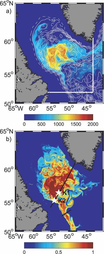
FIG. 1. (a) Simulated mixed layer depth (m; color shading) su- ries approximately the same transport mj ; that is, a
perimposed on barotropic streamfunction (Sv; isolines) during large (small) amount of drifters is deployed in section
March and (b) concentration of the idealized ventilation tracer in segments with large (small) cross-section velocities fol-
the range 27.77–27.80 kg m⫺3 during May; (a) also shows the
lowing Blanke and Raynaud (1997).
chosen limits for the Labrador Sea region, i.e., the 52°N and the
43°W section, and (b) shows the LC section at about 53°N and the The instantaneous transport of ventilated water
WOCE AR7W section running across the deep Labrador Sea, as through the 53°N section then is the sum of all transport
well as the locations of moorings K1 and K2 (white stars).
950 JOURNAL OF PHYSICAL OCEANOGRAPHY VOLUME 37
values assigned to those drifters passing through the Let H(x, y, t) be the isopycnal layer thickness, calcu-
section at a given time that were found to originate in lated as the water column height between two given
the mixed layer that same year. This transport can be bounds; then the following conservation equation
directly compared to the transport calculated using Eq. holds:
(3). While the mean transport of ventilated water
through the section obtained from the different meth- ⭸H
⫹ h · 共vhH兲 ⫽ S, 共4兲
ods is almost the same, both distributions differ as the ⭸t
ventilation tracer is affected by horizontal and vertical
where t is time, h · is the horizontal divergence opera-
diffusion, while the Lagrangian drifters are not.
tor, vh is the vertically averaged horizontal velocity vec-
tor in a potential density range with thickness H, and S
3) SUBDUCTION OF LSW is a source term including effects due to surface buoy-
Once the pathways of ventilated water have been ancy fluxes, diapycnal diffusion in the interior, nonlin-
calculated, the question of where the water leaves the earities in the equation of state, as well as numerical
mixed layer can be addressed. Similar to the subduction inaccuracies. We define a transformation rate T in a
process in the subtropics, responsible for the formation region that includes all the aforementioned effects by
of water masses in the permanent thermocline, we de- simply integrating S over the surface area of that re-
fine here subduction as the process in which a water gion. Both terms on the left-hand side of Eq. (4) are
particle leaves the mixed layer and is separated from calculated using daily model output fields. Annual
air–sea fluxes. Subduction is calculated using the back- mean volume change and horizontal divergence are cal-
ward trajectories of Lagrangian drifters deployed at the culated for different regions by integrating both terms
53°N section. The occurrence of subduction is identi- on the left-hand side of Eq. (4) over the surface area of
fied in time and space when the respective backward the regions, then averaging over time.
trajectory enters the mixed layer. Backward drifter tra- Assuming that the spatial mean change of isopycnal
jectories are calculated until the end of the year or until layer thickness within the entire Labrador Sea (north of
they reach the 50°N or 40°W section. However, only 52°N and west of 43°W) during a year is zero (i.e.,
5% of subduction occurs outside the tracer initializa- model in quasi-steady state), the annual mean transfor-
tion area. Using this method and the deployment strat- mation rate is given by
具 冖 H ds典,
egy described above, only subduction of water leaving
the Labrador Sea within the deep LC is considered. T⫽ 共5兲
⊥
The area of the Labrador Sea is divided into hori-
zontal grid boxes. We define an instantaneous subduc-
where ⊥ is the velocity component of perpendicular
tion rate (on a daily basis) within a horizontal grid box
to the line segment, ds, along the sections delimiting the
as the sum of all transport values assigned to drifters
Labrador Sea with an orientation westward along 52°N
subducted within this box. Note that the annual mean
(southern boundary, Fig. 1a), and northward along
subduction rate, that is, the mean over the analyzed
43°W (western boundary, Fig. 1a). The brackets in Eq.
year, in the entire model domain equals the annual
(5) represent the annual mean. The eastern and north-
mean transport of ventilated water through the 53°N
ern model boundaries of the Labrador Sea are closed.
section as calculated from the backward trajectories.
In this case the annual mean transformation rate equals
the annual mean net export out of the Labrador Sea for
4) WATER MASS TRANSFORMATION
a given class.
The question that we want to address here is: Where In addition to the effective transformation rate de-
does the water mass transformation take place? We will termined as the sum of local volume change and hori-
discuss two quantities: 1) an effective simulated water zontal divergence for a given class, we also calculate
mass transformation that includes all effects capable of a transformation rate from buoyancy fluxes at the
changing the water density in the model and 2) the ocean surface, a method originally pioneered by Speer
water mass transformation due to the model’s buoy- and Tziperman (1992). Here, we apply a similar method
ancy flux that captures the essential physics of surface that considers only the effect of negative surface buoy-
flux-driven convection. While the first transformation ancy flux on the oceanic stratification. The buoyancy
rate is evaluated for large boxes, the second one is cal- flux is defined to be negative when the resulting buoy-
culated at each grid point yielding detailed information ancy of the oceanic surface layer decreases. Starting
on where and when water mass transformation does from heat and freshwater fluxes, as well as temperature
occur. and salinity profiles for each horizontal grid box, the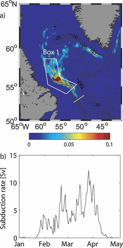
APRIL 2007 BRANDT ET AL. 951
local transformation from lighter into denser water due intense convection was found in particular in the early
to negative surface buoyancy fluxes is calculated. Here, 1990s. On the other hand, significantly shallower con-
daily model output fields are used. First, the change in vection depths were observed from 1998 to 2002 (La-
temperature and salinity in the uppermost grid box due zier et al. 2002; Stramma et al. 2004). The distribution
to daily heat and freshwater fluxes is calculated. The of the idealized ventilation tracer after the convection
convection scheme described by Rahmstorf (1993) is period during May (Fig. 1b) shows that a large part of
applied to completely remove static instability in the LSW in the potential density range ( ⫽ 27.77–27.80
water column and to obtain vertically homogeneous sa- kg m⫺3) was part of the mixed layer in the same year.
linity and potential temperature profiles in the mixed The distribution suggests that the main export route of
layer. ventilated LSW is via the deep LC.
After calculating from the initial temperature and The maximum of the annual mean overturning
salinity profiles and the profiles obtained by applying streamfunction as function of depth (equivalent to the
the daily surface freshwater and heat fluxes in conjunc- vertical volume transport) calculated along the sections
tion with the convection scheme, isopycnal layer thick- at 52°N, 43°W is 3.0 Sv. This value is larger than the
nesses are calculated for initial and obtained profiles value of 1.3 Sv reported by Böning et al. (1996). A
for the different classes. The difference between the larger vertical volume flux must be associated with a
initial and obtained layer thicknesses of the respective larger horizontal circulation (Spall and Pickart 2001).
classes defines the daily generation/destruction of In fact, the maximum barotropic streamfunction in the
layer thickness of a particular class due to negative Labrador Sea of about 55 Sv (Fig. 1a) is found to be at
surface buoyancy fluxes. The daily generated/destroyed the upper end of those described in a model compari-
isopycnal layer thicknesses are then summed up for dif- son study by Treguier et al. (2005), ranging from 40 to
ferent periods in time (e.g., months or seasons). The 60 Sv for different models.
transformation rate due to negative buoyancy flux, Tb⫺, With respect to many characteristics, such as flow
is obtained by integrating the generated/destroyed field and distribution of eddy kinetic energy (EKE), the
layer thicknesses of a particular class over the sur- present model is similar to the model of Eden and Bön-
face area of the respective region and division by the ing (2002). In their model solution as well as in the
time step (1 day). model solution presented here, a strong early winter
While we focus only on the effect of negative buoy- EKE maximum within the WGC as well as a smaller
ancy forcing, the calculation of water mass transforma- late winter EKE maximum in the region of the deep LC
tion presented here is similar to the approach suggested can be found. This is in general agreement with the
by Speer and Tziperman (1992). However, the present analysis of altimetric data (Lilly et al. 2003; Brandt et al.
scheme accounts for strongly varying (and particularly 2004).
large) mixed layer depths, which vary on horizontal and Recent direct velocity measurements at the exit of
temporal scales of the mesoscale eddy field. This rep- the Labrador Sea show a well-defined, mainly barotro-
resents a first approach calculating transformation rates pic deep boundary current and a weak recirculation
of LSW due to surface buoyancy fluxes in high- farther offshore (Fischer et al. 2004, their Fig. 5). The
resolution eddy-resolving models. observed structure of the Labrador Sea boundary cur-
rent is, in general, well represented by the model simu-
c. General characteristics of the model solution in
lations (Fig. 2). The top-to-bottom southeastward
the Labrador Sea
transport of the boundary current at 53°N is very simi-
In this study we focus on one 1-yr climatological lar, about 40 Sv and 38 Sv for simulated and observed
simulation with the regional model described in section boundary current transports, respectively. However,
2a. However, the calculations regarding the water mass the simulated southeastward transport of LSW in the
transformation are repeated for another climatological depth range ⫽ 27.74–27.8 kg m⫺3 is 19 Sv, which is
simulation using the FLAME Atlantic model with an clearly above the observed value of about 11 Sv for
open southern boundary shifted toward 18°S with very summer 1997–99 (Fischer et al. 2004). This can partly
similar results. be attributed to slightly shallower depths of simulated
The climatologically forced model experiment with isopycnal surfaces. At the offshore part of this section,
the regional model simulates a year of moderate con- the potential density surface ⫽ 27.74 kg m⫺3, typi-
vection intensity in the Labrador Sea with maximum cally used to separate upper LSW from classical LSW,
mixed layer depths of about 1600 m in March (Fig. 1a). is observed to be at about 600 m during summer 1996
Similar mixed layer depths were found in the Labrador and about 900 m during summer 1999. In the model
Sea for example, in 1997 (Pickart et al. 2002). More experiment presented here, the depth of this potential
952 JOURNAL OF PHYSICAL OCEANOGRAPHY VOLUME 37
FIG. 2. July mean 53°N section of alongshore velocity (cm s⫺1;
dashed contours denote southeastward velocities, and solid con-
tours northwestward velocities) superimposed on potential den-
sity (thin solid contours). Transport values are given for marked
layers bounded by zero isotach. The position of the slanted
section is marked in Fig. 1b. The dotted line separates the two
layers of LSW used in this study.
density surface is about 800 m in the offshore region
with a strong isopycnal doming up to a depth of 200 m
between the boundary current and the offshore recir-
culation (Fig. 2). Simulated doming, in excess of the
observed one, is related to stronger southeastward ve-
locities of the boundary current and stronger north-
westward velocities of the recirculation in the near- FIG. 3. (a) Simulated salinity (color shading) during June su-
surface flow, together with slightly narrower current perimposed on potential density (solid lines) along the WOCE
bands. Some of these differences might be also due to AR7W section marked in Fig. 1b. (b) Depth-averaged salinity of
the fact that the observations of Fischer et al. (2004) are the upper 700 m from data collected along WOCE AR7W section
taken during a period of weak convection in the Labra- in May 1997 (R/V Hudson) and July 1997 (R/V Meteor), and
corresponding simulated salinities from the previous FLAME
dor Sea, while the climatological model forcing simu- model (dashed lines) and the present model (solid lines).
lates convection of moderate intensity.
In most recent models, including the previous 1/12° The simulated and observed temporal evolution of
FLAME version analyzed in Eden and Böning (2002), the temperature field at the two mooring positions K1
simulated LSW potential density ranges differ consid- and K2 marked in Fig. 1b are shown for the period
erably from observed ranges (Treguier et al. 2005). This January to May (Fig. 4). The observational data corre-
fact complicates a direct comparison of observational spond to the year 1997. While the simulated tempera-
and modeling results with respect to the hydrographic ture in the boundary current in particular is larger than
structure of the Labrador Sea. Compared to those mod- observations indicate (note the different color scales
els, the simulated hydrographic structure of the model in Fig. 4), the structure of the temporal variability at
version at hand is substantially improved. The simu- the two positions agrees quite well. At mooring posi-
lated salinity along the World Ocean Circulation Ex- tion K1, representing the central Labrador Sea re-
periment AR7W section (Fig. 3a) shows a similar pat- gime, a continuous deepening of the mixed layer is
tern as described by Stramma et al. (2004) and Pickart observed only disturbed by single eddy events. Note
and Spall (2007). There is a deep salinity maximum at that the mixed layer deepening is slightly faster in the
about 2000-m to 2500-m depth and increased salinities model compared to the data. At mooring position K2,
in the WGC and LC below the near-surface layer. How- representing the boundary current regime, a strongly
ever, the depth-averaged salinity of the present model variable temperature field is found as the result of an
is, although reduced compared to previous model simu- intense eddy field advected along the boundary current
lations (Treguier et al. 2005), still larger than the ob- in both simulation and observation, while the mean
served salinities (Fig. 3b). wintertime cooling of the upper 500-m boundary cur-
APRIL 2007 BRANDT ET AL. 953
FIG. 4. Evolution of (a), (b) simulated and (c), (d) observed
potential temperature (°C) at mooring positions (a), (c) K1 and
(b), (d) K2 marked in Fig. 1b. The observations are from 1997.
Note the different temperature scales.
rent waters is weaker in the model compared to the
data.
We conclude that the simulated flow field and hydro-
graphic structure are within or close to observed
ranges. In the following, we apply different methods to
identify pathways of ventilated water masses as well as
to calculate ventilation and transformation rates. The
water mass definition for LSW is chosen as the isopy-
cnal range ⫽ 27.74–27.80 kg m⫺3, similar to that used
in observational studies (e.g., Fischer et al. 2004). We
FIG. 5. Ratio of annual mean ventilated water transport to an-
will further separate the LSW layer into an upper layer nual mean transport at the 53°N section marked in Fig. 1b (color
defined by ⫽ 27.74–27.77 kg m⫺3 and a lower layer de- shading) as obtained (a) from backward Lagrangian drifter tra-
fined by ⫽ 27.77–27.80 kg m⫺3 (cf. Fig. 2 and Fig. 3a). jectories and (b) from the idealized ventilation tracer. Also in-
cluded are annual mean alongshore velocities (cm s⫺1; black con-
tours, where dashed contours denote negative velocities, solid
3. Pathways of ventilated water masses
contours are positive velocities, and thick solid contours are zero
The export of ventilated water within the depth velocity) and selected isopycnal depths, (kg m⫺3; thick white
range of LSW mainly occurs in the deep LC. Only a contours). Transport values in (a) are given for annual mean
transport and annual mean transport of ventilated water for se-
minor contribution to the total export of ventilated
lected layers bounded by the zero isotach.
LSW leaves the Labrador Sea across the 43°W section.
This is illustrated in the May concentration of the ven-
tilation tracer within the isopycnal range ⫽ 27.77– (sum of transport values assigned to drifters that origi-
27.80 kg m⫺3 showing high tracer concentration up to nate in the mixed layer) to annual mean transport for
0.8 in the deep LC and low tracer concentration east of each section segment. Owing to the small number of
43°W (Fig. 1b). In the following we will investigate this drifters, the ratio is not well defined for very small
main export route of LSW using backward Lagrangian cross-sectional velocities (Fig. 5a).
drifter trajectories. The annual mean relative contribution of such ven-
By calculating Lagrangian trajectories of drifters de- tilated LSW to the southeastward transport of LSW at
ployed at the 53°N section in the deep LC backward in 53°N is about 60% for the upper LSW layer and about
time until 1 January using daily velocity fields, we con- 40% for the lower LSW layer (Fig. 5a). The distribution
firm that a large part of the total southeastward trans- of the ventilation tracer at the 53°N section (Fig. 5b)
port of LSW leaving the Labrador Sea at 53°N origi- shows a pattern similar to the distribution of ventilated
nates in the mixed layer that same year. The distribu- water from the Lagrangian drifter calculations. The
tion of ventilated water at the 53°N section is illustrated main differences are the smoother shape and slightly
by the ratio of annual mean ventilated water transport broader pattern in the case of the ventilation tracer.
954 JOURNAL OF PHYSICAL OCEANOGRAPHY VOLUME 37
FIG. 6. Time series of southeastward LSW transport and venti-
lated LSW transport across the slanted 53°N section (see Fig. 1b)
for different classes as obtained from backward Lagrangian
drifter trajectories.
These differences are attributed to the fact that the
distribution of the ventilation tracer is subject to verti-
cal and horizontal diffusion, while the Lagrangian path-
ways are purely obtained from advection using daily
velocity fields.
The southeastward transport of LSW at 53°N has a
seasonal transport maximum in February/March. Ven-
tilated LSW as obtained from Lagrangian drifter calcu-
lations is exported out of the Labrador Sea beginning in
February within the upper LSW layer and in March
within the lower LSW layer (Fig. 6). The large transport
values in winter demonstrate a rapid export of newly
ventilated LSW along the western boundary pathway,
starting as early as the convection period. The relative
contribution of ventilated LSW shows a near-steady de- FIG. 7. Subduction of LSW ( ⫽ 27.74–27.80 kg m⫺3) leaving
crease after the early export peak with a slight second- the Labrador Sea within the deep LC across the 53°N section
ary maximum in May. At the end of the year, about (thick white solid line) as obtained from backward Lagrangian
30% of the southeastward LSW export still consists of drifter trajectories: (a) spatial pattern of subduction velocity
(mm s⫺1; color shading) overlaid on annual mean barotropic
LSW that was part of the mixed layer during that same
streamfunction (Sv; black contours) and (b) time series of sub-
year. duction rate in box 1 marked in (a).
From the backward drifter trajectories the subduc-
tion rate of LSW is calculated as explained in section
tral Labrador Sea (Fig. 8). The buoyancy flux is calcu-
2b. The subduction rate is divided into different
lated using the heat flux defined by Eq. (1) (see section
classes according to the value of the drifter at the
2a) and the freshwater flux resulting from the restoring
53°N section. The subduction velocity (Fig. 7a) is cal-
of sea surface salinities to Levitus data. In general,
culated by dividing the subduction rate of each hori-
there is a stronger buoyancy loss over the deep LC
zontal grid cell by its surface area. The largest annual
relative to the central Labrador Sea. This is associ-
mean subduction velocities are found in the region
ated with strong air–sea temperature differences over
around 56°N, 56°W within the deep LC. The time series
the deep LC, particularly due to the upward mixing of
of the subduction rate within Box 1 shows that at this
heat originating from the IC that imports relatively
location subduction starts early in the year with a total
warm and salty waters at intermediate depths into the
maximum in March/April (Fig. 7b).
Labrador Sea. In the WGC, mostly anticyclonic eddies
are generated, which are capped by a layer of cold and
4. Water mass transformation less salty coastal waters. The shedding of these eddies
In the model, the mean wintertime buoyancy fluxes results in a reduction of the buoyancy flux along the
are characterized by strong buoyancy losses in the cen- eddy migration pathways into the interior Labrador
APRIL 2007 BRANDT ET AL. 955
FIG. 9. January (a) thickness changes of isopycnal layers defined
by given -bounds due to negative surface buoyancy flux, (b)
mean meridional velocity (cm s⫺1; color shading, white contours
FIG. 8. Mean January–April buoyancy flux (m2 s⫺3; color denote zero velocity) overlaid on potential density (black con-
shading) superimposed on mean January–April barotropic tours), and (c) total buoyancy flux (solid line) and buoyancy flux
streamfunction (Sv; black contours). Also shown is the 56.5°N due to heat flux only (dashed line). All quantities are plotted
section crossing the LC and central Labrador Sea (thick solid along 56.5°N marked in Fig. 8.
line).
layer thicknesses, in some areas much larger than the
Sea. Note that these relatively small-scale variations of
layer thickness of a particular potential density class,
the buoyancy flux (Fig. 8) are generated by the differ-
can only be obtained by a rapid export of the trans-
ence between simulated SST and climatological values
formed water masses. Thus, this transformation has
[Eq. (1)]. A comparison between satellite SST and
to occur in a region where the deep LC transports
model simulation (Emery et al. 2006) reveals in general
water southeastward out of the Labrador Sea (Fig. 9).
good agreement, in particular with respect to variations
At the same time, lighter and particularly warmer water
in the boundary currents. However, it is difficult to as-
masses are continuously imported into the region of
sess the realism of the buoyancy flux since there is
water mass transformation.
clearly a lack of surface flux data acquired during win-
During March, the water mass transformation area
ter capable of resolving the high temporal and spatial
becomes broader and reaches farther east (Fig. 10).
variability in the area.
In the following, we will discuss the water mass trans-
formation along a zonal section at 56.5°N, chosen for its
location directly north of the main subduction region.
The surface buoyancy forcing is dominated by the
buoyancy flux due to surface heat flux, and the fresh-
water flux contributes less than 10% to the total forcing
in general (Figs. 9 and 10). The water mass transforma-
tion, presented here as a change of isopycnal layer
thickness, commences in January with the transforma-
tion of water with ⫽ 27.68–27.77 kg m⫺3 into water
with ⫽ 27.77–27.80 kg m⫺3. This early transfor-
mation occurs in the transition region between the
boundary current and interior Labrador Sea. Here, the
stratification is considerably weaker compared to the
strongly stratified shallow LC farther onshore (Fig. 9b).
Within this region, the buoyancy loss is at its maximum
and a slight doming of the isopycnals (in particular ⫽
27.74 kg m⫺3) is observed. Large values of generated FIG. 10. As in Fig. 9 but for March.956 JOURNAL OF PHYSICAL OCEANOGRAPHY VOLUME 37
FIG. 12. Time series (10-day low-passed) of local volume change
(solid line), horizontal divergence (dotted line), transformation
rate due to negative surface buoyancy flux (dashed line), and
residual (dashed–dotted line) within box 1 marked in Fig. 11 for
⫽ 27.77–27.80 kg m⫺3.
27.80 kg m⫺3 associated with the transformation of
denser water masses (Fig. 11b).
For two boxes, as well as for the entire Labrador Sea,
the transformation rates due to negative buoyancy flux
are compared to the local volume change and horizon-
tal divergence [see section 2b, Eqs. (4) and (5)]. While
Box 1 represents the near–boundary current regime of
the deep LC, Box 2 represents the central Labrador Sea
regime with deepest mixed layer depths during winter
(Fig. 11). The residual marked in Figs. 12 and 13 is then
the sum of the local volume change and horizontal di-
vergence (effective transformation rate) minus the
transformation rate due to negative buoyancy flux. This
residual accounts for other transformation rates, that is,
FIG. 11. (a) January and (b) January–March thickness changes
(m) of isopycnal layer ⫽ 27.77–27.80 kg m⫺3 due to negative
due to positive surface fluxes, diapycnal diffusion, non-
surface buoyancy flux (color shading) superimposed on barotro- linearities in the equation of state, as well as numerical
pic streamfunction (Sv: black contours). Also included are box 1 inaccuracies. In particular, this residual may be due to
and box 2 representing the near–boundary current regime and the assumption made for the calculation of the trans-
central Labrador Sea regime, respectively. formation rate due to negative buoyancy flux; that is,
the buoyancy fluxes act on a given stratification for a
However, strongest transformation rates are obtained whole day, neglecting in this way effects of lateral/ver-
at the offshore flank of the deep LC. The regional dis- tical advection/diffusion in the model capable of chang-
tribution of simulated water mass transformation indi- ing the stratification during a day. The annual means of
cates the early start of water mass generation with ⫽ local volume change, horizontal divergence, and trans-
27.77–27.80 kg m⫺3 predominantly in the southern part formation rate due to negative buoyancy flux (Sv) for
of the Labrador Sea at about 55°W near the deep LC the three regions and different isopycnal layers are
(Fig. 11a). During the first three months of the year given in Table 1, where the sum of the first two columns
within the southern part of the Labrador Sea, more of each region represents the effective annual mean
than 3000–m layer thickness of water with ⫽ 27.77– transformation rate of the model. Positive values in
27.80 kg m⫺3 is generated locally. In the central Labra- Table 1 are associated with the volume increase of a
dor Sea, negative transformation rates indicate a de- potential density class in the respective region. Note
struction of layer thickness of water with ⫽ 27.77– that the annual-mean local volume change for all po-APRIL 2007 BRANDT ET AL. 957
tive buoyancy fluxes for the isopycnal layer ⫽ 27.77–
27.83 kg m⫺3 of Box 1 indicates that the transformation
starts in mid-January and leads initially to a local vol-
ume change of that isopycnal layer (Fig. 12). The export
of this water mass out of Box 1, which is represented by
the horizontal divergence, starts at the beginning of
February with maximum values in March/April. The
export rapidly decreases with the end of negative buoy-
ancy fluxes and associated water mass transformation
in mid-April (Fig. 12).
In the central Labrador Sea (Box 2) the negative
buoyancy fluxes lead to the generation of water with
⫽ 27.77–27.80 kg m⫺3 from the end of January to the
beginning of February, and directly results in an in-
crease of the simulated volume of that isopycnal layer
(Fig. 13a). Throughout the year, the horizontal diver-
gence is weak, nevertheless yielding an almost continu-
ous export out of Box 2 between May and October.
During March/April, negative transformation rates are
obtained that are associated with the generation of
denser water masses. Similarly, these denser water
masses ( ⫽ 27.80–27.83 kg m⫺3) are continuously ex-
ported out of Box 2 between May and October (Fig.
13b). In summary, strongest water mass transformation
rates are obtained in the near–boundary current box
(Box 1). The export out of this box is already at a
maximum during the convection period, indicating a
rapid exit pathway of transformed water masses within
the deep LC. The export of transformed water masses
FIG. 13. As in Fig. 12 but for Box 2 marked in Fig. 12; from the central Labrador Sea (Box 2) is a slow process,
(a) ⫽ 27.77–27.80 kg m⫺3 and (b) ⫽ 27.80–27.83 kg m⫺3. continuing over several months. We have checked the
robustness of the obtained results by analyzing also a
different eddy-resolving model realization based on the
tential density classes is rather small, indicating that last year of a 10-yr spinup of a basin-scale version of the
the model is approximately in a quasi-steady state FLAME model. The comparison between both model
(Table 1). realizations shows that the distribution of the transfor-
From the annual-mean transformation rates due to mation rate is very similar (cf. Fig. 11b and Fig. 14).
negative buoyancy flux (Table 1), we conclude that This similarity applies consequently to Figs. 8–13. It
about one-third of the LSW transformation for ⫽ suggests that in climatological simulations the internal
27.77–27.80 kg m⫺3 occurs in Box 1, while about two- year-to-year variability of the annual mean transforma-
thirds of LSW transformation is spread over large parts tion rate is small.
of the Labrador Sea (Fig. 11b). In Box 2, the annual
mean transformation rates are smaller, but denser wa-
5. Summary and discussion
ter masses ( ⫽ 27.80–27.83 kg m⫺3) are also gener-
ated here. From the horizontal divergence, we find a Ventilation, transformation, and export of LSW have
net inflow into Box 1 of water with potential density been investigated using a numerical simulation per-
of ⬍ 27.74 kg m⫺3 and a net outflow of water with formed with an eddy-resolving model of the subpolar
⫽ 27.74–27.80 kg m⫺3, while for Box 2, we find a North Atlantic with climatological forcing. The model
net inflow of water with ⬍ 27.77 kg m⫺3 and corre- realistically describes some salient features of the cir-
spondingly a net outflow of water with ⫽ 27.77–27.83 culation in the subpolar North Atlantic: most of the
kg m⫺3. analyzed model characteristics fall within or are close to
The temporal evolution of local volume change, hori- the range of observed characteristics. The chosen
zontal divergence, and transformation rate due to nega- model experiment represents a year of moderate con-958 JOURNAL OF PHYSICAL OCEANOGRAPHY VOLUME 37
TABLE 1. Annual-mean local volume change, horizontal divergence, and water mass transformation rate due to negative surface
buoyancy fluxes for different classes for the entire Labrador Sea limited by the 52°N and the 43°W sections (Fig. 1a), the
near-boundary current region (Box 1), and the central Labrador Sea (Box 2, see Fig. 11): Units are Sverdrups.
Labrador Sea Box 1 Box 2
Local Local Local
volume Horizontal Transformation volume Horizontal Transformation volume Horizontal Transformation
class change divergence rate change divergence rate change divergence rate
⬍27.68 ⫺0.2 ⫺3.3 ⫺4.7 0.0 ⫺0.1 ⫺0.5 0.0 ⫺0.1 ⫺0.2
27.68–27.74 0.2 ⫺3.1 ⫺3.9 0.0 ⫺1.5 ⫺1.8 ⫺0.1 ⫺0.4 ⫺0.4
27.74–27.77 0.0 1.2 1.5 0.0 0.2 0.2 ⫺0.1 ⫺0.7 ⫺0.7
27.77–27.80 0.1 5.0 6.4 0.1 1.4 2.1 0.1 0.7 0.7
27.80–27.83 ⫺0.2 0.6 0.7 0.0 ⫺0.1 0.0 0.1 0.5 0.7
⬎27.83 0.1 ⫺0.4 0.0 0.0 0.1 0.0 ⫺0.1 0.1 0.0
vection intensity with March mixed layer depths of they derived mixed layer depths in late winter/early
about 1600 m. spring and compared them with the observed profiles.
We distinguish between transformation rate and ven- Starting with a profile at the position of mooring B1244
tilation rate. The effective transformation rate of the in the deep LC (see Fig. 14 for its location), they were
model is calculated as the sum of local volume change not able to simulate any significant mixed layer deep-
and horizontal divergence for a given isopycnal layer, ening. Starting with a profile that is advected cycloni-
Eq. (4). Additionally, the transformation rate due to cally around the Labrador Sea, from the northern La-
negative surface buoyancy fluxes is calculated based on brador Sea to the position of mooring B1244, they ob-
a method originally proposed by Speer and Tziperman tained good agreement between simulated and
(1992). It is found that LSW is predominantly trans- observed profiles, confirming the importance of water
formed at the offshore flank of the deep LC. mass transformation along the deep LC pathway as sug-
The ventilation rate is calculated by applying two gested in Figs. 11b and 14.
methods: 1) an idealized ventilation tracer and 2) back-
ward Lagrangian drifter trajectories. Both methods are
used to describe the temporal evolution and export
pathways of newly ventilated LSW. The main export
route of ventilated LSW in the present model simula-
tion is the deep LC (Fig. 1b). From backward drifter
calculations, we find that about 50%, or 9.2 Sv, of LSW
leaving the Labrador Sea at 53°N within the deep LC
originates in the mixed layer that same year (Fig. 5a).
The subduction of mixed layer water leaving the La-
brador Sea within the deep LC is found to occur mainly
in the southern part of the Labrador Sea during the
convection period (Fig. 7).
By evaluating Eq. (4), we find in the near-boundary
current box a maximum volume change for the lower
part of LSW (27.77 ⬍ ⬍ 27.80 kg m⫺3) in early
February. The maximum volume change coincides with
the onset of strong LSW transformation as inferred
from negative buoyancy fluxes. The LSW transforma-
tion peaks in February/March (Fig. 12). The simulated
early start of LSW transformation within the near–
boundary current region agrees well with recent find-
ings of an observational study by Cuny et al. (2005),
FIG. 14. January–March thickness changes (m) of isopycnal
who have done a detailed analysis of heat fluxes and
layer ⫽ 27.77–27.80 kg m⫺3 due to negative surface buoyancy
mixed layer depths in the Labrador Sea based on ob- flux (color shading) superimposed on barotropic streamfunction
served CTD profiles and moored stations. Using early (Sv: black contours) for the FLAME Atlantic model. Also in-
winter density profiles and applying air–sea heat fluxes, cluded are mooring positions K2, B1244, and K1.APRIL 2007 BRANDT ET AL. 959
When interpreting hydrographic sections, mainly
taken during summer, it is important to know how
quickly transformed water is flushed out of the Labra-
dor Sea and what is the seasonal cycle of the trans-
formed water export. In our model analysis we find
that the export of transformed LSW out of the near-
boundary current box (given by its horizontal diver-
gence) undergoes a strong seasonal cycle, with maxi-
mum export rates in February/March and high values
until May (Fig. 12). Accordingly, the analysis of back-
ward Lagrangian trajectories yields maximum south-
eastward export of newly ventilated LSW across the
53°N section at about the same time (Fig. 6). Both
analyses suggest a rapid export of transformed/venti-
lated LSW out of the Labrador Sea made possible due
to the proximity of the main water mass transformation
region to the deep LC. In contrast, water masses trans-
formed in the central Labrador Sea are exported more
slowly (Fig. 13).
The picture drawn by the model appears consistent
with the recent analysis of observational data by Pickart
et al. (2002). They suggested two types of water mass
products: 1) the classical “gyre product” transformed
seaward of the deep LC and 2) a “boundary product”
transformed in the deep LC approximately near the
2500-m depth contour where the alongshore velocity is
O(10 cm s⫺1). The dynamical role of the boundary cur-
rent in water mass transformation, hardly to be esti-
mated from data alone, was studied by Spall (2004)
using a model of an idealized marginal sea. He found a
main temperature balance in the model boundary cur-
rent between the warming due to mean advection and
cooling due to surface heat loss and lateral eddy fluxes.
The resulting downwelling in his model is located
within a narrow boundary layer over the sloping bot-
tom and at the offshore flank of the boundary current.
The present model, while principally in agreement with
that distribution, refines this picture by allowing infer-
ences about the transformation and ventilation patterns
in a realistic Labrador Sea setting.
The differences between transformation and ventila- FIG. 15. (a) Annual mean cross-sectional transport and (b) an-
tion rates, defined by Eqs. (5) and (3), can clearly be nual mean cross-sectional transport of ventilated water for differ-
seen by accumulating annual mean isopycnal transport ent classes accumulated along the sections at 52°N and 43°W
marked in Fig. 1a, starting at the coast of Labrador at 52°N, 56°W.
and isopycnal transport of ventilated water along the
The straight vertical dashed lines mark the corner at 52°N, 43°W.
52°N and 43°W sections limiting the Labrador Sea (Fig. Also given in (a) and (b) are annual mean transformation rates, T
15). There is a net annual mean inflow into the Labra- [Eq. (5)], and annual mean ventilation rates, FA [Eq. (3)], in the
dor Sea of lighter water ( ⬍ 27.74 kg m⫺3) of 6.4 Sv Labrador Sea for different classes, respectively.
and of denser overflow waters ( ⬎ 27.83 kg m⫺3) of
0.4 Sv. Water within the potential density range 27.74 ⬍
⬍ 27.83 kg m⫺3 is net exported out of the Labrador discussed before, besides the main export of ventilated
Sea, yielding a transformation rate of 6.8 Sv (Fig. 15a). LSW in the deep LC, there is only a minor contribution
Ventilated water is exported out of the Labrador Sea in to the total export of ventilated LSW by the export
all potential density classes with ⬍ 27.83 kg m⫺3. As across the 43°W section (Fig. 15b).960 JOURNAL OF PHYSICAL OCEANOGRAPHY VOLUME 37
The annual mean export rate of ventilated LSW of the basis for the present simulations. The model inte-
about 10 Sv is larger than the annual mean transforma- grations were performed at the German Climate Com-
tion rate of LSW (6.3 Sv) calculated as the sum of local puting Centre (DKRZ), Hamburg, Germany.
volume change and horizontal divergence (Table 1).
This means that the exported LSW contains more water REFERENCES
that originates in the mixed layer that same year than
was generated by water mass transformation. While we Arakawa, A., and V. R. Lamb, 1977: Computational design of the
find good agreement between ventilation and transfor- basic dynamical processes of the UCLA general circulation
mation rates for the higher potential density classes model. Methods Comput. Phys., 17, 173–265.
⫽ 27.77–27.83 kg m⫺3 (giving some confidence in the Barnier, B., L. Siefridt, and P. Marchesiello, 1995: Thermal forc-
ing for a global ocean circulation model using a three-year
chosen mixed layer criterion), for all lighter density
climatology of ECMWF analyses. J. Mar. Syst., 6, 363–380.
classes, in particular for upper LSW ( ⫽ 27.74–27.77 Beckmann, A., and R. Döscher, 1997: A method for improved
kg m⫺3), ventilation rates are larger than transforma- representation of dense water spreading over topography in
tion rates (cf. Fig. 15a and 15b). geopotential-coordinate models. J. Phys. Oceanogr., 27, 581–
To understand this apparent contradiction, consider 591.
a case of zero water mass transformation. In such a case Blanke, B., and S. Raynaud, 1997: Kinematics of the Pacific equa-
the amount of water mass generated is the same as the torial undercurrent: An Eulerian and Lagrangian approach
from GCM results. J. Phys. Oceanogr., 27, 1038–1053.
amount of water mass destroyed. Although there is no
Böning, C. W., F. O. Bryan, W. R. Holland, and R. Döscher, 1996:
change in volume, part of the water mass could have Deep-water formation and meridional overturning in a high-
been in contact with the atmosphere and, thus, venti- resolution model of the North Atlantic. J. Phys. Oceanogr.,
lated accordingly. Therefore differences between trans- 26, 1142–1164.
formation and ventilation rates are present, in particu- Boyer, T. P., and S. Levitus, 1997: Objective Analysis of Tempera-
lar for those water masses that are partially trans- ture and Salinity for the World Ocean on a 1⁄4 Degree Grid.
NOAA Atlas NESDIS 11, 62 pp.
formed into denser water masses during winter. This
Brandt, P., F. A. Schott, A. Funk, and C. S. Martins, 2004: Sea-
holds also for long-term averages. This result is impor-
sonal to interannual variability of the eddy field in the La-
tant for the analysis of CFC inventories, an observa- brador Sea from satellite altimetry. J. Geophys. Res., 109,
tional tool for ventilation rates. Our results suggest, for C02028, doi:10.1029/2002JC001551.
example, that during years of classical LSW generation, Cuny, J., P. B. Rhines, F. Schott, and J. Lazier, 2005: Convection
transformation rates of upper LSW derived from CFC above the Labrador continental slope. J. Phys. Oceanogr., 35,
measurements would be overestimated. 489–511.
Last, caveats regarding a possible overestimate of the Czeschel, L., 2004: The role of eddies for the deep water forma-
tion in the Labrador Sea. Ph.D. thesis, Leibniz-Institut für
near-boundary current effects in the model are related
Meereswissenschaften an der Universität Kiel, 95 pp.
to the structure of the boundary current. In fact, the
Döös, K., 1995: Interocean exchange of water masses. J. Geophys.
simulated boundary current appears stronger than ob- Res., 100, 13 499–13 514.
served, and proximity of the boundary current and re- Eden, C., and C. Böning, 2002: Sources of eddy kinetic energy in
circulation results in a stronger doming of isopycnals in the Labrador Sea. J. Phys. Oceanogr., 32, 3346–3363.
between than observed (Fischer et al. 2004). In addition Emery, W. J., P. Brandt, A. Funk, and C. Böning, 2006: A com-
the simulated boundary current is associated with parison of sea surface temperatures from microwave remote
slightly warmer and saltier waters at intermediate sensing of the Labrador Sea with in situ measurements and
model simulations. J. Geophys. Res., 111, C12013,
depths than observations indicate. However, there is a
doi:10.1029/2006JC003578.
large year-to-year variability in the hydrographic struc-
Fischer, J., and F. A. Schott, 2002: Labrador Sea Water tracked by
ture of the boundary current, and the obtained results profiling floats—From the boundary current into the open
can be seen as an exemplary case describing the differ- North Atlantic. J. Phys. Oceanogr., 32, 573–584.
ent processes relevant for the ventilation, transforma- ——, ——, and M. Dengler, 2004: Boundary circulation at the exit
tion, and export of LSW during a specific year. of the Labrador Sea. J. Phys. Oceanogr., 34, 1548–1570.
Khatiwala, S., P. Schlosser, and M. Visbeck, 2002: Rates and
Acknowledgments. This work was supported by the mechanisms of water mass transformation in the Labrador
Sea as inferred from tracer observations. J. Phys. Oceanogr.,
German Science Foundation (DFG) as part of the
32, 666–686.
‘‘Sonderforschungsbereich’’ SFB 460 ‘‘Dynamics of
Kieke, D., M. Rhein, L. Stramma, W. M. Smethie, D. A. LeBel,
Thermohaline Circulation Variability.’’ We thank F. and W. Zenk, 2006: Changes in the CFC inventories and
Schott, J. Fischer, and M. Dengler for helpful discus- formation rates of upper Labrador sea water, 1997–2001. J.
sions. The authors acknowledge the model develop- Phys. Oceanogr., 36, 64–86.
ment efforts of the Kiel FLAME group that provided Lavender, K. L., R. E. Davis, and W. B. Owens, 2000: Mid-depthYou can also read


