A Socially Aware Huff Model for Destination Choice in Nature-based Tourism
←
→
Page content transcription
If your browser does not render page correctly, please read the page content below
AGILE: GIScience Series, 2, 14, 2021. https://doi.org/10.5194/agile-giss-2-14-2021
Proceedings of the 24th AGILE Conference on Geographic Information Science, 2021.
Editors: Panagiotis Partsinevelos, Phaedon Kyriakidis, and Marinos Kavouras.
This contribution underwent peer review based on a full paper submission.
© Author(s) 2021. This work is distributed under the Creative Commons Attribution 4.0 License.

A Socially Aware Huff Model for Destination Choice in
Nature-based Tourism
Meilin Shia,b (corresponding author), Krzysztof Janowicza,b , Ling Caia,b , Gengchen Maia,b and Rui
Zhua,b

meilinshi@ucsb.edu, janowicz@ucsb.edu, lingcai@ucsb.edu, gengchen_mai@ucsb.edu, ruizhu@ucsb.edu

a
    STKO Lab, Department of Geography, University of California, Santa Barbara, USA
b
    Center for Spatial Studies, University of California, Santa Barbara, USA

Abstract. Identifying determinants of tourist destina-
tion choice is an important task in the study of nature-
based tourism. Traditionally, the study of tourist be-
havior relies on survey data and travel logs, which
are labor-intensive and time-consuming. Thanks to
location-based social networks, more detailed data is
available at a finer grained spatio-temporal scale. This
allows for better insights into travel patterns and in-
teractions between attractions, e.g., parks. Meanwhile,
such data sources also bring along a novel social influ-
ence component that has not yet been widely studied
in terms of travel decisions. For example, social influ-
encers post about certain places, which tend to influ-
ence destination choices of tourists. Therefore, in this
paper, we propose a socially aware Huff model to ac-
count for this social factor in the study of destination
choice. Moreover, with fine-grained social media data,
interactions between attractions (i.e., the neighboring
effects) can be better quantified and thus integrated into
models as another factor. In our experiment, we cali-
brate a model by using trip sequences extracted from
geotagged Flickr photos within two national parks in
the United States. Our results demonstrate that the so-
cially aware Huff model better simulates tourist travel
preferences. In addition, we explore the significance of
each factor and summarize the spatial-temporal travel
pattern for each attraction. The socially aware Huff
model and the calibration method can be applied to
other fields such as promotional marketing.

Keywords. nature-based tourism, socially aware Huff
model, tourist destination choice, geotagged social me-
dia, Flickr

                          Reproducibility review: https://doi.org/10.17605/osf.io/4cpm3           1 of 16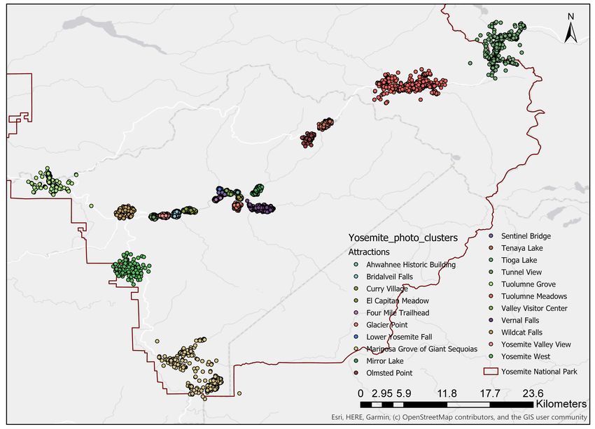
1       Introduction                                                   be used to quantify visitation rates (Wood et al., 2013),
                                                                       to estimate visitor flows (Orsi and Geneletti, 2013;
Nature tourism, i.e., tourism that is based on the natural             Kim et al., 2019), and to detect popular sub-regions
attractions of an area, has gone through rapid growth                  and temporal activity patterns (Heikinheimo et al.,
over the past two decades (Balmford et al., 2009), es-                 2017). These studies illustrate the capability of using
pecially for national parks in the United States, ac-                  LBSNs to capture temporal variations in tourist visit-
cording to visitation statistics by National Park Ser-                 ing, with some places (e.g., dive resorts) being more at-
vice. 1 Identifying and evaluating relevant determinants               tractive in summer and others (e.g., ski resorts) in win-
of tourist flows is important. On the one hand to pro-                 ter. In addition, interactions between places (i.e., the
mote tourism, and on the other hand it helps to pro-                   neighboring effects) can be better quantified with so-
tect natural lands. Prior work on nature-based tourism                 cial media data. For example, we can estimate the inter-
relies on manually collected travel logs and survey                    actions between Horseshoe Bend and those attractions
data, which are time-consuming, labor-intensive, and                   in its surroundings (Glen Canyon, Antelope Canyon,
limited in temporal coverage (Puustinen et al., 2009;                  Grand Canyon, etc.), based on which we can further
Nahuelhual et al., 2013). The emergence of location-                   explore how they affect potential travel decisions of
based social networks (LBSNs) and volunteered geo-                     tourists to Horseshoe Bend, thereby uncovering inter-
graphic information (VGI), such as Flickr, Instagram,                  esting travel patterns that are difficult to detect using
Facebook etc., together with geotagging technology,                    traditional data.
provides more fine-grained spatial and temporal data,                  To explore how social factors and neighboring effects
which equips us with a new lens to understand travel                   contribute to tourist destination choice in natural at-
patterns as they relate to natural attractions.                        tractions, we propose a socially aware version of the
Additionally, LBSNs play an increasingly important                     well-known Huff model (Huff, 1964), which was orig-
role in travel decision making process (Leung et al.,                  inally used to calculate the probability of a customer
2013). For example, places like Horseshoe Bend,                        shopping at each retail store.
Devil’s Bathtub, etc., once being hidden gems, are                     The contributions of this work are as follows:
now receiving a large number of visitors annually.
Social media has been regarded as the main culprit                       • We propose a socially aware Huff model, which
for the sudden and overwhelming popularity of these                        incorporates both social factors and neighboring
places (Djossa, 2019). More specifically, geotagged                        effects, to estimate the probability of tourists vis-
photos posted by social media influencers (SMIs) can                       iting specific places.
rapidly attract new visitors (Glover, 2009). These in-
fluencers are usually users with a large number of fol-                  • The proposed method is calibrated on a data set
lowers and have established credibility in certain fields                  containing 10-year geotagged Flickr photos in
that can shape attitudes of tourists and thus influencing                  two national parks, whose results outperform the
their travel preferences (Freberg et al., 2011; Li, 2016).                 baseline Huff model.
Intuitively, a scenic photo posted by a user with 50k
followers has a much broader potential influence than                    • We explore the spatial and temporal variability of
a user with 50 followers. Therefore, we argue that so-                     model parameters that are associated with attrac-
cial factors brought by increasingly used social media                     tiveness, distance, and neighboring effect in the
need to be taken into account as a new norm to comple-                     socially aware Huff model.
ment traditional destination choice models. To justify
such an argument, we specifically explore this social                  The remainder of this paper is organized as follows.
effect in nature-based tourism destination choices, be-                Section 2 introduces related work on tourism, geo-
cause tourists tend to share geotagged photos on social                social media, and the Huff model. Section 3 briefly in-
media platforms along their trips (Tasse et al., 2017).                troduces the Flickr data set used for the study and ex-
                                                                       plains the trip reconstruction process. A socially aware
Moreover, existing work has shown that fine-grained
                                                                       Huff model is introduced in section 4 together with the
spatio-temporal data collected from social media can
                                                                       model calibration method. In section 5, we present the
    1
        https://irma.nps.gov/Stats/                                    model calibration results and explain the spatial and

AGILE: GIScience Series, 2, 14, 2021 | https://doi.org/10.5194/agile-giss-2-14-2021                                      2 of 16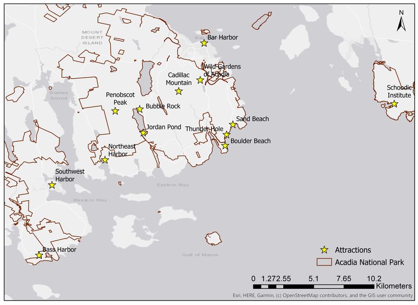
temporal variability of the parameters used in the so-                 lau and Más, 2008; Wu et al., 2012; Yang et al.,
cially aware Huff model. Finally, we summarize our                     2013). The Huff model (Huff, 1964) is one of them,
findings and discuss future directions in section 6.                   though it was originally developed to predict retail
                                                                       sales and consumer behavior. The Huff model esti-
                                                                       mates the probability of consumer patronizing retail
2     Related Work                                                     stores based on two factors: attractiveness of a store
                                                                       and travel cost, which can also be applied to tourism
                                                                       research. Misui and Kamata (2016) adopted the Huff
2.1   Tourism and Geo-social Media                                     model to show the effect of travel time on visiting prob-
                                                                       ability to spa destinations in Japan. Similarly, Nicolau
The use and role of social media has been widely dis-                  (2008) studied tourist sensitivities to distance and price
cussed in tourism research (Leung et al., 2013). Work                  for destination choice in Spain using a national tourist
by Zheng et al. (2012) used Flickr data to discover                    choice behavior survey data. Yang et al. (2013) con-
regions of attractions (RoAs) and explored tourists                    ducted a logistic model to study the inter-dependencies
movement patterns in relation to the RoAs. Simi-                       among destination choices when two or more desti-
larly, Hu et al. (2019) extracted popular attractions and              nations are included in a trip, accounting for the fu-
tour routes using a graph-based network in New York                    ture dependency in the multi-destination choice behav-
City from Twitter data. Majid et al. (2013) proposed                   iors. Recently, more work has shown the importance
a context-aware personalized travel recommendation                     of the temporal factor that is missing in the original
system and evaluated it based on a Flickr data set.                    Huff Model. Gong et al. (2020) included weekday and
Li et al. (2018) used Flickr data to compare the spa-                  weekend variations when calculating visiting probabil-
tial overlap of tourists’ and locals’ destinations in ten              ity of shopping areas using taxi trajectory data in Shen-
US cities. Work by Mou et al. (2020) analyzed spatio-                  zhen and New York. Liang et al. (2020) proposed a T-
temporal distribution and changes of inbound tourism                   Huff model and proved that it outperforms the original
flow in Shanghai with Flickr data.                                     static Huff model when estimating temporal store visits
In the past decade, social media has evolved into an                   using SafeGraph POI visits data. Likewise, we include
important player in tourism advertising and promo-                     the temporal factor in our study given the availability
tion (Bakr and Ali, 2013). Litvin et al. (2008) showed                 of social media data.
that travelers are increasingly influenced by electronic
Word-of-Mouth (eWOM) from social media. Parsons
(2017) echoed the similar idea that Instagram influ-                   3         Data and Trip Reconstruction
ences tourist decision-making, especially for younger
generations. Jalilvand and Samiei (2012) examined the
                                                                       In this section, we introduce the data set used for the
influence of eWOM and showed that it has a signifi-
                                                                       study in section 3.1 and explain how we reconstruct
cant impact on tourist attitudes towards visiting Isfa-
                                                                       trips from the geotagged photos step by step in sec-
han, Iran. Tham et al. (2020), however, conducted in-
                                                                       tion 3.2.
terviews with tourist decision-makers in Australia and
revealed that social media’s role appears to have only
moderate-low influence on destination choice. In line                  3.1        Data and Study Area
with such research, we include a social influence factor
and examine the impact of social media on destination                  In this study, we collected geotagged Flickr photos of
choices. We quantify the social impact that influencers                tourist attractions within national parks using Flickr’s
could bring to a place by measuring the place attrac-                  public API. 2 Two national parks - Acadia National
tiveness given the travel preference of tourists.                      Park and Yosemite National Park - have been selected
                                                                       from the top ten most visited national parks in the
2.2   Huff Model                                                       United States over the past decade, as reported by Na-
                                                                       tional Park Service. These geotagged Flickr photos
                                                                       were collected from January 1, 2010 to December 31,
There have been many research efforts towards tourist
                                                                             2
destination choice and sequential tourist flows (Nico-                           https://www.flickr.com/services/api/

AGILE: GIScience Series, 2, 14, 2021 | https://doi.org/10.5194/agile-giss-2-14-2021                                       3 of 16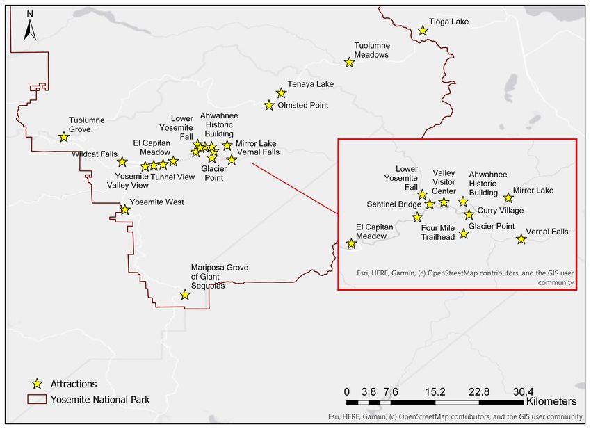
2019. Each photo is associated with its metadata in- 3.2.2 Extracting trip sequences from geotagged
cluding photo ID, owner ID, taken date, latitude, longi- photos
tude, title, and the number of views. The total numbers
of the geotagged Flickr photos and unique users in the With attractions being identified, each photo in the
data set are summarized in Tab. 1. cluster is labeled with an attraction name (or cluster
ID). To extract trip sequences, we first group all pho-
Table 1 The numbers of geotagged Flickr photos and
tos by their owner ID and then sort them by the date
unique users retrieved for this study.
taken. We consider a trip as a temporally-ordered se-
Park Number of photos Number of users quence of photographed locations taken by the same
Acadia NP 34,933 1,879 user. Given the possibility that one user could make
Yosemite NP 50,384 3,653 several trips to the area over the years, we set a time
threshold λt to distinguish these trips. If the time dif-
ference between two consecutive photos from the same
3.2 Trip Reconstruction user is larger than λt , we separate them into two differ-
ent trips. Here, we set λt to 4 days, which is the aver-
age length of a stay in both national parks according to
3.2.1 Identifying attractions using HDBSCAN
National Park Statistics. 4, 5
Spatial clustering is widely applied to point pattern Thus, if a user took a photo at attraction A, attraction
analysis such as hot spot detection. One of the most B, and then attraction C within the λt constraint, we are
popular clustering methods is DBSCAN (Ester et al., able to capture this trip sequence as [A, B, C] based on
1996), which is a density-based clustering algorithm. the timestamp of each geotagged Flickr photo. For our
It requires two parameters: search radius () and min- data set, 1,949 trip sequences were extracted from the
imum number of points (minPts) within the search ra- clustered geotagged photos in Acadia National Park,
dius. Despite its broad applications, it is difficult to de- and 3,426 trip sequences from Yosemite National Park.
termine the in the original DBSCAN algorithm due
to varying density distributions of points. In this paper,
we adopt HDBSCAN (Campello et al., 2013; McInnes
et al., 2017), a hierarchical density-based clustering al-
3.2.3 Calculating visiting probabilities from trip
gorithm, which addresses the aforementioned issue by
sequences
using flexible values to identify attractions from the
geotagged Flickr photos.
With the trip sequences extracted, we are able to con-
To identify a proper value for MinClusterSize, we com-
struct a flow matrix based on the trip segments from
pare different clustering results with the geographic
all trip sequences. For example, [A, B] and [B, C] are
distribution of top attractions listed on TripAdvisor 3 in
two trip segments from the trip sequence [A, B, C].
the two national parks. Based on this comparison, Min-
The visiting probability is calculated proportional to
ClusterSize is set to 1% of the total number of photos,
the total number of outgoing trips for each attraction in
which is 349 and 504 for Acadia and Yosemite Na-
the flow matrix. A monthly visiting probability matrix
tional Parks, respectively.
is also calculated in order to capture temporal factors
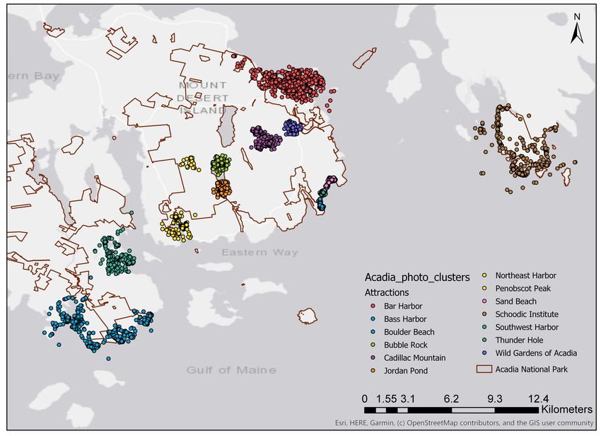
After applying the HDBSCAN algorithm, 13 clusters in later computations. Fig. 2 visualizes the overall trip
are extracted from Acadia National Park and 21 clus- flows in the two national parks using flowmap.blue. 6
ters from Yosemite National Park. We calculate the Further details of each attraction are provided in Tab. 8
centroids of the clusters and label each cluster with and Tab. 9.
the nearest attraction listed on TripAdvisor or Google
Maps to its centroid coordinates. Fig. 1 shows the dis-
tribution of geotagged photos, clustering results, as 4
https://www.nps.gov/acad/planyourvisit/faqs.htm
well as the identified attraction names of Acadia and 5
https://www.nps.gov/yose/learn/management/statistics.
Yosemite National Parks. htm
3 6
https://www.tripadvisor.com/ https://flowmap.blue/
AGILE: GIScience Series, 2, 14, 2021 | https://doi.org/10.5194/agile-giss-2-14-2021 4 of 16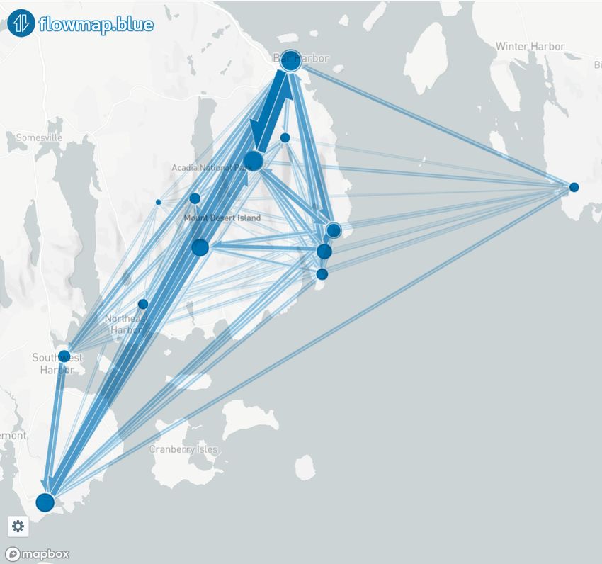
(a) Acadia National Park

                                                    (b) Yosemite National Park

Figure 1. Photo clusters detected by HDBSCAN in the two national parks.

AGILE: GIScience Series, 2, 14, 2021 | https://doi.org/10.5194/agile-giss-2-14-2021   5 of 16
4 A Socially Aware Huff Model
In this paper, we leverage the Huff model (Huff,
1964) with multi-destination travel behaviors being
taken into account (Stouffer, 1940; Um and Cromp-
ton, 1990). Fig. 3 is used to illustrate the neighboring
effect in a multi-destination trip. In Fig. 3(a), a tourist
at Origin O has two destination choices A and B, with
equal distance to origin O. In this case, destination B
should be preferred since it has more future choices
in its neighborhood compared with destination A. Fur-
thermore, Fig. 3(b) illustrates the effect of attractive-
ness. When destination A and B have the same number
of future choices in their neighborhood and the same
distance to Origin O, then intuitively the destination
with more attractive future choices in its neighborhood
would be preferred. Orpana and Lampinen (2003) used
the term “store centralities” to model the effect of its
neighboring outlets on a store’s utility. The term can
be interpreted as the possibility of interaction between
(a) Acadia National Park a store and its neighbors (Hansen, 1959). The “cen-
trality” concept is applied to model tourist destination
choice as well, with the assumption that people tend to
travel to places with more attractive future choices.
4.1 The Original Huff Model
The original Huff Model (Huff, 1964) is designed to
estimate the probability of customers at each origin pa-
tronizing a given store among all stores as their desti-
nation choices. It takes two factors into account: attrac-
tiveness and distance. Attractiveness can be computed
as a function of many attributes of a store, including
the store size, number of parking spaces, customer re-
views, etc. The classic form of the Huff model can be
expressed as:
(b) Yosemite National Park β
Aα
j Dij
Pij = Pn (1)
α β
Figure 2. Flow map visualization of trips in the two national j=1 Aj Dij
parks. Attractions are represented as nodes. The size of nodes
is determined by the total number of incoming and outgoing
trips. The width of edges is determined by the number of where Pij represents the probability of a customer at
trips. location i visiting store j; Aj is the measure of attrac-
tiveness of store j; Dij is the distance between location
i and store j; and n indicates the total number of stores
in the data set. The parameters α and β (α >0, βdescribe the neighboring effect of attraction j, relative
to other attractions at time t; and n indicates the total
number of attractions in the area. The parameters α, β
and θ are associated with the attractiveness, distance,
and neighboring effect factors, respectively.
In the following, we explain how we quantify the three
terms, i.e., Ajt , Djt , and Cjt , mathematically. Previ-
ous research has shown that the number of geotagged
photos and the number of unique users can be used
to represent the attractiveness of a place (Kádár and
(a) Different number of future choices for desti- Gede, 2013; Leung et al., 2017). Here, we include three
nation A and B.
proxies to estimate the attractiveness Ajt for later com-
parison. Log transformation is performed to address a
right-skewed distribution of values. The three types of
(l)
attractiveness Ajt , l = 1, 2, 3, can be expressed as:
(1)
Ajt = log(Mjt + 1) (3)
where Mjt is the number of photos at attraction j at
time t.
(2)
Ajt = log(Ujt + 1) (4)
(b) Same number of future choices for destina-
tion A and B. Circle size represents the measure where Ujt is the number of unique users at attraction j
of attractiveness. at time t.
Figure 3. Diagram of future choices in multi-destination
travel behavior. Mjt
(3) 1 X
Ajt = log(Mjt × Vkjt + 1) (5)
Ujt
4.2 Socially Aware Huff Model k=1
where Vkjt is the number of views for photo k at attrac-
In this paper, we propose a socially aware Huff model tion j at time t. We use the product of the number of
to include social factor and neighboring effect, based photos and the average number of photo views per user
on the assumptions that: (1) People tend to choose at attraction j to include a social influence factor. Given
more attractive travel destinations; (2) People tend to the fact that social media influencers (SMIs) have more
choose closer travel destinations; (3) People tend to followers than others, thus the photos they post would
choose travel destinations with more beneficial future have more views and greater social impact, we include
choices. Based on the original Huff model shown in photo views per user here to account for potential exis-
Eq. 1, the socially aware Huff model can be expressed tence of SMIs who upload photos at an attraction. We
as: hypothesize that the attraction with more photo views
per user is more attractive.
β θ The term Cjt , measuring the neighboring effect, can be
Aαjt Dij Cjt
Pijt = Pn (2) modeled as:
α β θ
j=1 Aj Dij Cjt PK Akt
k=1 Dkj
Cjt = PK (6)
where Pijt represents the probability of a tourist at lo- 1
k=1 Dkj
cation i visiting attraction j at time t; Ajt is the attrac-
tiveness of attraction j at time t; Dij is the distance be- where K is the total number of nearest neighboring at-
tween origin i and attraction j; Cjt is the term used to tractions being considered. Cjt reflects the assumption
AGILE: GIScience Series, 2, 14, 2021 | https://doi.org/10.5194/agile-giss-2-14-2021 7 of 16that people tend to travel to places with more promis- 4.4 Software and Data Availability
ing future choices in a multi-destination trip. We con-
sider K-nearest neighbors of attraction j, calculating Data used in this paper can be accessed with the public
(l)
their attractiveness Akt at time period t, and weight Flickr API. 8 The query used to access the data, code
(l)
Akt by their distance to attraction j, Dkj . A higher Cjt and interactive data visualization (Fig. 2) are avail-
value is assigned to attractions with closer and more at- able on GitHub. 9 The workflow underlying this paper
tractive neighbors. Finally, we define the term Dij as was partially reproduced by an independent reviewer
the estimated driving distance using the Distance Ma- during the AGILE reproducibility review and a repro-
trix API 7 from Google Maps. ducibility report was published at https://doi.org/10.
17605/OSF.IO/4CPM3.
4.3 Calibration Method
Parameters of the Huff model need to be calibrated 5 Results and Discussions
before further studying the travel patterns. Here, we
use the linear regression calibration method - Ordi- 5.1 Overall Calibration Results
nary Least Squares (OLS), which estimates one set of
parameters α, β, and θ, that best fit the model based
on observations. The estimation process is executed In this section, we examine the overall calibration re-
by minimizing the sum of squared residuals in a lin- sults for the two national parks and discuss the neces-
ear model. OLS calibration returns fixed values for the sity of incorporating social factors and neighboring ef-
parameters and assumes that they are homogeneous fects in the socially aware Huff model.
across the study area. The general form of OLS regres-
sion can be expressed as: 5.1.1 K-Nearest Neighbors
n
X First we need to decide on the number of neighbors K
y= βi xi + (7) in order to calculate the centrality Cjt in Eq. 6. Val-
i=1
ues of K = 2, 3 and 5 are considered. For both Acadia
and Yosemite National Parks, K = 2 gives the best per-
where y is the dependent variable; xi is the ith inde- formance, with the lowest mean squared error (MSE)
pendent variable; n is the number of independent vari- and highest R2 . More details are shown in Tab. 7. The
ables; βi is the regression coefficient for the ith inde- following calibrations are subsequently all computed
pendent variable; and is the random error. with K = 2 as the number of nearest neighbors in the
To conduct OLS, the socially aware Huff model in centrality term Cjt .
Eq. 2 is rewritten in a log-transformed-centered form,
according to Nakanishi and Cooper (1974), in order to
5.1.2 Social Influence
obtain the least square estimate of parameters:
In Tab. 2, we show the calibration results using dif-
(l)
ln(Pijt /P˜it ) = αi ln(Ajt /Ãt ) ferent measurements of the attractiveness factor, Ajt ,
(8)
expressed in Eq. 3, Eq. 4 and Eq. 5. Based on R2 and
+ βi ln(Dij /D̃i ) + θi ln(Cjt /C̃t ) Akaike information criterion (AIC), we observe that
(3)
for both national parks, the attractiveness Ajt per-
where P˜it , A˜jt , D̃i and, C̃t are the means of Pijt ; Ajt ; forms the best (highest R2 and lowest AIC values),
Dij and Cjt over attraction j, respectively. For each compared with the other two measurements (i.e., the
origin attraction i, the model will estimate one best fit number of photos and the number of unique users).
parameter set (αi , βi , and θi ). 8
https://www.flickr.com/services/api/
9
https://github.com/meilinshi/
7
https://cloud.google.com/maps-platform/routes Socially-aware-Huff-model
AGILE: GIScience Series, 2, 14, 2021 | https://doi.org/10.5194/agile-giss-2-14-2021 8 of 16Table 2 OLS regression results for different measurements of attractiveness
Park Measurement of Attractiveness R2 AIC ∆AICi wi
(1)
Acadia NP Ajt 0.743 724.6 14.9 5.810 × 10⁻⁴
(2)
Ajt 0.741 728.1 18.4 1.010 × 10⁻⁴
(3)
Ajt 0.753 709.7 0 0.9993
(1)
Yosemite NP Ajt 0.715 2401.7 25.4 3.050 × 10⁻⁶
(2)
Ajt 0.717 2393.0 16.7 2.363 × 10⁻⁴
(3)
Ajt 0.721 2376.3 0 0.9998
∆AICi is a measure of each model i to the model
P with the minimum AIC.
Akaike weights wi = exp(−0.5 × ∆AICi )/ N r=1 exp(−0.5 × ∆AICr )
Table 3 OLS regression results for different factors considered
Park Model R2 AIC ∆AICi wi
Acadia NP SA model 0.753 709.7 0 0.9859
SA model w/o N 0.746 718.2 8.5 0.0141
SA model w/o T 0.744 748.5 38.8 3.703 × 10⁻⁹
Huff model 0.738 755.8 46.1 9.624 × 10⁻¹¹
Yosemite NP SA model 0.721 2376.3 1.3 0.3430
SA model w/o N 0.721 2375.0 0 0.6570
SA model w/o T 0.714 2412.4 37.4 4.969 × 10⁻⁹
Huff model 0.714 2410.6 35.6 1.222 × 10⁻⁸
∆AICi is a measure of each model i to the model with the minimum AIC. Models with ∆AICi < 2 can also be considered to
have substantial support (Burnham and Anderson,
P 2002).
Akaike weights wi = exp(−0.5 × ∆AICi )/ N r=1 exp(−0.5 × ∆AICr )
The results of Akaike weights (wi ), which can be in- includes both temporal factor and neighboring effect
terpreted as the probability that model i is the best has the highest R2 and lowest AIC values for Acadia
model (Anderson et al., 2000), also show the same National Park. As for Yosemite National Park, the per-
(3)
conclusion. Hence, we select Ajt to estimate the at- formance of SA model and SA model w/o N are sim-
tractiveness of an attraction, where the combination of ilar in terms of R2 and AIC, while both models fit to
photo views, the total number of photos, as well as the the data better than SA model w/o T and Huff model.
number of users are taken into account. The results However, we cannot conclude that SA model w/o N is
indicate that including a social factor (i.e., the more significantly better than SA model or vice versa based
photo views and potential social impact SMIs could on ∆AICi and wi values. The reason why we get sim-
bring to a place) can better simulate tourist preferences. ilar performance for SA model and SA model w/o N
may be due to the geographic distribution of attractions
in Yosemite National Park (see Fig. 4). Most attrac-
5.1.3 Temporal and Neighboring Effect Factors tions are clustered (i.e., they have similar neighbors)
at the center of the park, thus the neighboring effect
To examine the overall performance of the temporal may not be as significant as those of Acadia National
factor and neighboring effect in the socially aware Huff Park. More details about this will be discussed in sec-
model (SA model), we compare it with SA model tion 5.2. In general, the SA model w/o N performs bet-
without the neighboring effect (SA model w/o N), SA ter than the SA model w/o T, since the temporal factor
model without the temporal factor (SA model w/o T), provides more fine-grained data and for national parks,
and the original Huff model (Huff model), whose re- to include temporal variation when estimating visiting
sults are shown in Tab. 3. The proposed SA model that
AGILE: GIScience Series, 2, 14, 2021 | https://doi.org/10.5194/agile-giss-2-14-2021 9 of 16(a) Acadia National Park (b) Yosemite National Park
Figure 4. Geographic distribution of attractions in the two national parks.
patterns is crucial. Overall, the experimental results in- mations for attractions in Acadia National Park. Here,
dicate the necessity to incorporate both social and tem- we see a relatively small estimation of α for Cadillac
poral effects into the Huff model. Mountain, which is the top 1 traveler favorite attraction
in Acadia National Park ranked by TripAdvisor. This
5.2 Regional Variability of Parameters means that compared with visitors at Boulder Beach,
Sand Beach, and Jordan Pond etc., after visiting Cadil-
lac Mountain, they are less interested in the attractive-
After examining the globally fitted parameters for the ness of an attraction to visit the next destination. The
entire park, we further explore the regional variabil- absolute values of β estimations are greater for Bass
ity of the parameters. The intuition underlying this ex- Harbor and Bubble Rock, which indicate that visitors
periment is that the relative impacts of attractiveness tend to choose closer next destinations starting from
(α), distance (β), and neighboring effect (θ) can be these two attractions. A larger θ estimation indicates
different across regions in the park. Therefore, cali- a higher probability of visitors choosing destinations
bration is conducted for each attraction in the two na- with closer and more attractive neighbors, most likely
tional parks using observed visiting probabilities cal- clustered attractions, such as the Boulder Beach, Thun-
culated from the trip sequence data. Each attraction is der Hole and Sand Beach cluster (see Fig. 4(a)).
treated as an origin to estimate how visitors choose
their next destination starting from this origin attrac- Tab. 5 includes the parameter calibration results for
tion. The OLS calibration gives one set of parame- attractions in Yosemite National Park. We see rela-
ters (α, β, and θ) per origin, reflecting how attrac- tively larger estimations of α for attractions clustered
tiveness, distance and neighboring effect, respectively, at the center of the park, El Capitan Meadow, Lower
contribute to the visiting probabilities. The results for Yosemite Fall, Sentinel Bridge, etc., which are shown
attractions within Acadia and Yosemite National Parks in the red box of Fig. 4(b). The largest absolute value
are shown in Tab. 4 and Tab. 5. Only these significant of β estimation for Tuolumne Grove indicates that
origin attractions with more than 30 observed trips are visitors at this attraction are very likely to choose a
included in the table. closer next destination. Since Yosemite National Park
is roughly 15 times larger than Acadia National Park
In general, a large absolute estimation for α, β, or θ in area, absolute values of β estimations are gener-
indicates a significant influence of attractiveness, dis- ally smaller compared with those of attractions in Aca-
tance, or neighboring effect to the destination choices, dia National Park. This indicates visitors are less sen-
respectively. Tab. 4, demonstrates the parameter esti- sitive to distance and are willing to travel further in
AGILE: GIScience Series, 2, 14, 2021 | https://doi.org/10.5194/agile-giss-2-14-2021 10 of 16Table 4 OLS regression results for Acadia National Park Origin Attraction α β θ MSE R2 Bass Harbor 0.8863* -0.8608* 0.1155 0.273 0.731 Northeast Harbor 0.1684 -0.1137 0.4079* 0.208 0.838 Bar Harbor 1.3226*** 0.2359 -0.0224 0.322 0.739 Cadillac Mountain 0.6601 -0.0218 0.1907 0.360 0.707 Bubble Rock 0.1722 -0.4898* 0.3994* 0.322 0.791 Jordan Pond 1.5456*** -0.0670 -0.0133 0.203 0.886 Boulder Beach 2.0496*** 0.3590* -0.3446 0.334 0.751 Thunder Hole 1.2109** -0.1355 0.0232 0.301 0.782 Sand Beach 2.1061*** 0.0374 -0.3318 0.397 0.742 Significance level: ***p ≤ 0.001; **p ≤ 0 .01; *p ≤ 0 .05. Table 5 OLS regression results for Yosemite National Park Origin Attraction α β θ MSE R2 Mariposa Grove of Giant Sequoias 1.6864*** -0.1023 -0.1060 0.433 0.743 Tioga Lake 1.4482* 0.0467 0.0381 0.770 0.615 Tuolumne Grove 0.7325* -1.1656** 0.4270*** 0.368 0.850 Tuolumne Meadows 0.8987** -0.4552*** 0.0985 0.388 0.776 Olmsted Point 0.2791 -0.0827 0.3661** 0.399 0.731 Tenaya Lake 0.9528* -0.3699*** 0.0838 0.495 0.786 Wildcat Falls 1.6585*** -0.0451 -0.0818 0.355 0.799 Mirror Lake 1.8888*** -0.0490 -0.2065 0.343 0.802 Vernal Falls 0.9077*** -0.0532 0.0236 0.294 0.666 El Capitan Meadow 1.1824*** -0.1147 0.0205 0.208 0.827 Tunnel View 0.5004 -0.2491 0.1451 0.368 0.646 Bridalveil Falls 1.3182*** 0.0177 -0.1471 0.216 0.736 Yosemite Valley View 0.9467** -0.2522** 0.0218 0.253 0.844 Glacier Point 1.3761*** 0.0131 0.0563 0.500 0.703 Curry Village 1.3791*** -0.0800 -0.1009 0.281 0.781 Four Mile Trailhead 1.5207*** -0.0087 -0.1623* 0.168 0.836 Ahwahnee Historic Building 1.0631*** -0.1871* 0.0486 0.333 0.795 Valley Visitor Center 1.0149*** -0.0792 -0.0690 0.197 0.743 Lower Yosemite Fall 1.2195*** -0.0022 -0.0135 0.200 0.803 Sentinel Bridge 1.2127*** -0.1188** -0.1572** 0.182 0.827 Significance level: ***p ≤ 0.001; **p ≤ 0 .01; *p ≤ 0 .05. Yosemite National Park. The estimation of parame- Mile Trailhead, Bridalveil Falls, Sentinel Bridge, etc., ter θ is greater for dispersed attractions like Olmsted that are already in a clustered region. For origin attrac- Point and Tuolumne Grove, as can be seen in Fig. 4(b). tions with θ closer to 0, it means that neighboring effect This means visitors at these two attractions are more is not an important factor for visitors to choose their attracted to clustered attractions (i.e. attractions with next destination at these places. closer and more attractive neighbors), most likely the Tunnel View and Glacier Point clusters as shown in 5.3 Temporal Variability of Parameters the map. In Tab. 5, we also see significant negative θ values, which reveal that visitors tend to travel to less clustered attractions (i.e., attractions with further and To further explore the temporal variability of the model less attractive neighbors), especially for visitors at Four parameters, we divide the trips in Yosemite National AGILE: GIScience Series, 2, 14, 2021 | https://doi.org/10.5194/agile-giss-2-14-2021 11 of 16
Table 6 OLS regression results for Yosemite National Park Summer vs. Non-Summer months
 Origin Attraction                    Time of the year      α                   β                 θ                 R2
 Wildcat Falls                        Summer                1.7046*             0.0519            -0.1768           0.744
                                      Non-summer            1.4516*             -0.1670           0.0945            0.859
 Vernal Falls                         Summer                0.8962**            -0.1116*          -0.0355           0.679
                                      Non-summer            0.9788***           0.0379            0.0978            0.693
 El Capitan Meadow                    Summer                1.2480***           -0.0869           0.0372            0.918
                                      Non-summer            1.0437**            -0.2023           0.0010            0.768
 Tunnel View                          Summer                0.4185              -0.4669*          0.1651            0.756
                                      Non-summer            0.7634              -0.0111           0.1197            0.607
 Bridalveil Falls                     Summer                1.4542***           0.1098            -0.1979           0.729
                                      Non-summer            0.9029              -0.1969           -0.0592           0.755
 Curry Village                        Summer                1.3597***           -0.0117           -0.0348           0.800
                                      Non-summer            1.2933***           -0.2013**         -0.1963*          0.800
 Valley Visitor Center                Summer                0.8253***           -0.0782           -0.0404           0.705
                                      Non-summer            1.1169***           -0.0841           -0.0643           0.784
 Lower Yosemite Fall                  Summer                1.1861***           0.0315            0.0102            0.841
                                      Non-summer            1.2295***           -0.0319           -0.0319           0.787
 Sentinel Bridge                      Summer                0.7097*             -0.2088**         -0.0307           0.779
                                      Non-summer            1.4738***           -0.0374           -0.1927**         0.875

   Significance level: ***p ≤ 0.001; **p ≤ 0 .01; *p ≤ 0 .05. Summer months include May, June, July, August, and September.

Park to summer and non-summer based on the park                         attractions in non-summer months. Meanwhile, we see
travel recommendation. 10 A couple of attractions in                    also larger absolute θ estimations for Curry Village
the park are seasonal, with many roads and trails being                 in non-summer months and Bridalveil Falls in sum-
closed due to snow in winter. For example, Tuolumne                     mer months. A positive θ estimation means visitors are
Meadows typically opens from late May or June to                        more attracted to clustered attractions (i.e., attractions
November and Glacier Point typically opens from May                     with closer and more attractive neighbors) and negative
to November. According to most travel guides, the best                  value means the opposite.
time to visit Yosemite is May to September. Hence, we
use this time range to represent summer months here,
and the rest as non-summer months. In Tab. 6, only ori-                 6   Conclusions and Future Work
gin attractions with more than 30 observed trips during
both time periods are included.
                                                                        In this work, we explore the visiting probabilities of
Based on Tab. 6, we observe that the α estimations                      attractions within two national parks using a socially
mostly stay the same for different times of the year.                   aware Huff model, in which both social factors and
However, visitors at Bridalveil Falls are more sensi-                   neighboring effects are taken into account. To cali-
tive to the attractiveness factor in summer months,                     brate the model parameters, we use the observed trip
while visitors at Sentinel Bridge are more interested                   sequences extracted from the geotagged Flickr pho-
in the attractiveness factor in non-summer months.                      tos within Acadia and Yosemite National Parks from
Attractions like Vernal Falls, Tunnel View, Sentinel                    the year 2010 to 2019. For the social factor, we have
Bridge, etc., show larger absolute values of β estima-                  shown that incorporating the number of photo views
tions in summer. This means visitors at these attrac-                   when evaluating the attractiveness of a place achieves
tions are attracted to closer attractions during the sum-               a better result than simply using the number of photos
mer months, and further attractions for non-summer                      or number of users alone. The calibration results also
months, which is potentially due to closures of closer                  demonstrate that the socially aware Huff model con-
                                                                        sidering a temporal factor in place attractiveness and
  10
       https://www.nps.gov/yose/planyourvisit/traffic.htm               neighboring effects is more accurate than the original

AGILE: GIScience Series, 2, 14, 2021 | https://doi.org/10.5194/agile-giss-2-14-2021                                       12 of 16
Huff model in predicting visiting probabilities of at- Notes in Artificial Intelligence and Lecture Notes in Bioin-
tractions within both national parks. formatics), pp. 160–172, Springer, Berlin, Heidelberg, 2013.
We further explore the visiting patterns of each at- Djossa, C.: When not to geotag while traveling, National Ge-
traction within the two national parks based on model ographic, 2019.
parameters of attractiveness, distance, and neighbor- Ester, M., Kriegel, H.-P., Sander, J., Xu, X., et al.: A density-
ing effect factors. In general, visitors in Acadia Na- based algorithm for discovering clusters in large spatial
tional Park are more sensitive to the distance factor databases with noise., in: Kdd, vol. 96, pp. 226–231, 1996.
and neighboring effects when choosing their next des- Freberg, K., Graham, K., McGaughey, K., and Freberg,
tination, while visitors in Yosemite National Park are L. A.: Who are the social media influencers? A study of pub-
more sensitive to the attractiveness factor. We have also lic perceptions of personality, Public Relations Review, 37,
shown that there is a regional and temporal variability 90–92, 2011.
of the model parameters. Glover, P.: Celebrity endorsement in tourism advertising:
This work is based on our three assumptions that: (1) Effects on destination image, Journal of Hospitality and
Tourism Management, 16, 16–23, 2009.
People tend to choose more attractive travel destina-
tions; (2) People tend to choose closer travel destina- Gong, S., Cartlidge, J., Bai, R., Yue, Y., Li, Q., and Qiu, G.:
tions; (3) People tend to choose travel destinations with Geographical and temporal huff model calibration using taxi
more beneficial future choices. In fact, there could be trajectory data, GeoInformatica, pp. 1–28, 2020.
many other factors contributing to the visiting proba- Hansen, W. G.: How Accessibility Shapes Land Use, Journal
bility of a place. Taking the social factor alone as an ex- of the American Planning Association, 25, 73–76, 1959.
ample, traveling under social influence or taking copy- Heikinheimo, V., Minin, E. D., Tenkanen, H., Hausmann, A.,
cat photos (Picheta, 2021) has become an emerging Erkkonen, J., and Toivonen, T.: User-Generated Geographic
trend. In future work, we plan to consider more com- Information for Visitor Monitoring in a National Park: A
prehensive measurements to evaluate the social impact Comparison of Social Media Data and Visitor Survey, ISPRS
of geotagged photos in order to better capture the travel International Journal of Geo-Information, 6, 85, 2017.
patterns. Furthermore, this work is only studied using Hu, F., Li, Z., Yang, C., and Jiang, Y.: A graph-based ap-
existing attractions within national parks. We plan to proach to detecting tourist movement patterns using social
look at more than just two parks in the future, explore media data, Cartography and Geographic Information Sci-
new methods to discover emerging travel destinations ence, 46, 368–382, 2019.
and study their interactions with the surroundings. Huff, D. L.: Defining and Estimating a Trading Area, Journal
of Marketing, 28, 34–38, 1964.
Jalilvand, M. R. and Samiei, N.: The impact of electronic
References word of mouth on a tourism destination choice: Testing the
theory of planned behavior (TPB), Internet Research, 22,
Anderson, D. R., Burnham, K. P., and Thompson, W. L.: Null 591–612, 2012.
hypothesis testing: problems, prevalence, and an alternative,
Kádár, B. and Gede, M.: Where Do Tourists Go? Visualizing
The journal of wildlife management, pp. 912–923, 2000.
and Analysing the Spatial Distribution of Geotagged Pho-
Bakr, G. and Ali, I. E. H.: The role of social networking sites tography, Cartographica: The International Journal for Geo-
in promoting Egypt as an international tourist destination, graphic Information and Geovisualization, 48, 78–88, 2013.
South Asian Journal of Tourism and Heritage, 6, 169–183,
Kim, Y., ki Kim, C., Lee, D. K., woo Lee, H., and Andrada,
2013.
R. I. T.: Quantifying nature-based tourism in protected ar-
Balmford, A., Beresford, J., Green, J., Naidoo, R., Walpole, eas in developing countries by using social big data, Tourism
M., and Manica, A.: A Global Perspective on Trends in Management, 72, 249–256, 2019.
Nature-Based Tourism, PLoS Biology, 7, e1000 144, 2009.
Leung, D., Law, R., Van Hoof, H., and Buhalis, D.: Social
Burnham, K. P. and Anderson, D. R.: A practical media in tourism and hospitality: A literature review, Journal
information-theoretic approach, Model selection and multi- of travel & tourism marketing, 30, 3–22, 2013.
model inference, 2, 2002.
Leung, R., Vu, H. Q., and Rong, J.: Understanding tourists’
Campello, R. J., Moulavi, D., and Sander, J.: Density-based photo sharing and visit pattern at non-first tier attractions via
clustering based on hierarchical density estimates, in: Lec-
ture Notes in Computer Science (including subseries Lecture
AGILE: GIScience Series, 2, 14, 2021 | https://doi.org/10.5194/agile-giss-2-14-2021 13 of 16geotagged photos, Information Technology and Tourism, 17, Parsons, H.: Does social media influence an individual’s de-
55–74, 2017. cision to visit tourist destinations? Using a case study of
Li, D., Zhou, X., and Wang, M.: Analyzing and visualizing Instagram., Ph.D. thesis, Cardiff Metropolitan University,
the spatial interactions between tourists and locals: A Flickr 2017.
study in ten US cities, Cities, 74, 249–258, 2018. Picheta, R.: New Zealand tells tourists to stop copying other
Li, Z.: Psychological empowerment on social media: who are people’s travel photos, CNN, 2021.
the empowered users?, Public Relations Review, 42, 49–59, Puustinen, J., Pouta, E., Marjo Neuvonen, and Tuija Sievä-
2016. nen: Visits to national parks and the provision of natural and
Liang, Y., Gao, S., Cai, Y., Foutz, N. Z., and Wu, L.: Cali- man-made recreation and tourism resources, Journal of Eco-
brating the dynamic Huff model for business analysis using tourism, 8, 18–31, 2009.
location big data, Transactions in GIS, 24, 681–703, 2020. Stouffer, S. A.: Intervening Opportunities: A Theory Relat-
Litvin, S. W., Goldsmith, R. E., and Pan, B.: Electronic word- ing Mobility and Distance, American Sociological Review,
of-mouth in hospitality and tourism management, Tourism 5, 845, 1940.
management, 29, 458–468, 2008. Tasse, D., Liu, Z., Sciuto, A., and Hong, J.: State of the geo-
Majid, A., Chen, L., Chen, G., Mirza, H. T., Hussain, I., tags: Motivations and recent changes, in: Proceedings of the
and Woodward, J.: A context-aware personalized travel rec- International AAAI Conference on Web and Social Media,
ommendation system based on geotagged social media data vol. 11, 2017.
mining, International Journal of Geographical Information Tham, A., Mair, J., and Croy, G.: Social media influence on
Science, 27, 662–684, 2013. tourists’ destination choice: importance of context, Tourism
McInnes, L., Healy, J., and Astels, S.: hdbscan: Hierarchical Recreation Research, 45, 161–175, 2020.
density based clustering, The Journal of Open Source Soft- Um, S. and Crompton, J. L.: Attitude determinants in tourism
ware, 2, 205, 2017. destination choice, Annals of Tourism Research, 17, 432–
Misui, Y. and Kamata, H.: Where do Spa tourists come 448, 1990.
from?-An application of Huff model to Japanese spa destina- Wood, S. A., Guerry, A. D., Silver, J. M., and Lacayo, M.:
tion, Tech. rep., University of Massachusetts Amherst, 2016. Using social media to quantify nature-based tourism and
Mou, N., Yuan, R., Yang, T., Zhang, H., Tang, J. J., and recreation, Scientific reports, 3, 1–7, 2013.
Makkonen, T.: Exploring spatio-temporal changes of city in- Wu, L., Zhang, J., and Fujiwara, A.: A Tourist’s Multi-
bound tourism flow: The case of Shanghai, China, Tourism Destination Choice Model with Future Dependency, Asia Pa-
Management, 76, 103 955, 2020. cific Journal of Tourism Research, 17, 121–132, 2012.
Nahuelhual, L., Carmona, A., Lozada, P., Jaramillo, A., and Yang, Y., Fik, T., and Zhang, J.: Modeling sequential tourist
Aguayo, M.: Mapping recreation and ecotourism as a cul- flows: Where is the next destination?, Annals of Tourism Re-
tural ecosystem service: An application at the local level in search, 43, 297–320, 2013.
Southern Chile, Applied Geography, 40, 71–82, 2013. Zheng, Y.-T., Zha, Z.-J., and Chua, T.-S.: Mining travel pat-
Nakanishi, M. and Cooper, L. G.: Parameter Estimation for a terns from geotagged photos, ACM Trans. Intell. Syst. Tech-
Multiplicative Competitive Interaction Model: Least Squares nol, 3, 2012.
Approach, Journal of Marketing Research, 11, 303, 1974.
Nicolau, J. L.: Characterizing Tourist Sensitivity to Distance,
Journal of Travel Research, 47, 43–52, 2008.
Appendix
Nicolau, J. L. and Más, F. J.: Sequential choice behavior: Go-
ing on vacation and type of destination, Tourism Manage-
Regression results with different K values selected
ment, 29, 1023–1034, 2008.
for K-NN
Orpana, T. and Lampinen, J.: Building Spatial Choice Mod-
els from Aggregate Data, Journal of Regional Science, 43,
319–348, 2003. Attractions Summary
Orsi, F. and Geneletti, D.: Using geotagged photographs and
GIS analysis to estimate visitor flows in natural areas, Journal
for Nature Conservation, 21, 359–368, 2013.
AGILE: GIScience Series, 2, 14, 2021 | https://doi.org/10.5194/agile-giss-2-14-2021 14 of 16Table 7 OLS regression results for different K values selected for K-Nearest Neighbors
Park Time of the year K MSE R2
Acadia National Park All time 2 0.351958 0.753
3 0.355672 0.750
5 0.360020 0.747
Summer months 2 0.239118 0.780
3 0.241003 0.778
5 0.241888 0.777
Non-summer months 2 0.470965 0.766
3 0.479230 0.762
5 0.490113 0.757
Yosemite National Park All time 2 0.373372 0.721
3 0.373495 0.721
5 0.373465 0.721
Summer months 2 0.310437 0.714
3 0.310878 0.714
5 0.311528 0.713
Non-summer months 2 0.430608 0.735
3 0.430768 0.734
5 0.431058 0.734
Summer months include May, June, July, August, and September for both parks.
Table 8 Summary of attractions in Acadia National Park
Attraction Number of photos Outgoing trips Incoming trips
Schoodic Institute 1119 53 64
Bass Harbor 2298 260 288
Southwest Harbor 723 109 111
Northeast Harbor 605 67 76
Bar Harbor 6259 433 357
Wild Gardens of Acadia 550 60 66
Cadillac Mountain 3285 349 345
Penobscot Peak 776 16 15
Bubble Rock 703 83 89
Jordan Pond 1250 227 250
Boulder Beach 536 85 102
Thunder Hole 977 167 185
Sand Beach 1253 216 177
AGILE: GIScience Series, 2, 14, 2021 | https://doi.org/10.5194/agile-giss-2-14-2021 15 of 16Table 9 Summary of attractions in Yosemite National Park Attraction Number of photos Outgoing trips Incoming trips Mariposa Grove of Giant Sequoias 1787 135 135 Tioga Lake 1054 111 111 Tuolumne Grove 555 65 53 Tuolumne Meadows 1630 151 165 Yosemite West 674 35 31 Olmsted Point 890 168 165 Tenaya Lake 626 123 128 Wildcat Falls 724 147 110 Mirror Lake 875 134 150 Vernal Falls 2349 205 229 El Capitan Meadow 1010 175 197 Tunnel View 1987 489 414 Bridalveil Falls 1835 366 332 Yosemite Valley View 1469 231 249 Glacier Point 2165 250 288 Curry Village 855 140 157 Four Mile Trailhead 1269 246 225 Ahwahnee Historic Building 560 91 107 Valley Visitor Center 1788 201 197 Lower Yosemite Fall 869 164 167 Sentinel Bridge 1194 267 284 AGILE: GIScience Series, 2, 14, 2021 | https://doi.org/10.5194/agile-giss-2-14-2021 16 of 16
You can also read