THE IMPACT OF INHOMOGENEOUS EMISSIONS AND TOPOGRAPHY ON OZONE PHOTOCHEMISTRY IN THE VICINITY OF HONG KONG ISLAND - MPG.PURE
←
→
Page content transcription
If your browser does not render page correctly, please read the page content below
Atmos. Chem. Phys., 21, 3531–3553, 2021
https://doi.org/10.5194/acp-21-3531-2021
© Author(s) 2021. This work is distributed under
the Creative Commons Attribution 4.0 License.

The impact of inhomogeneous emissions and topography on ozone
photochemistry in the vicinity of Hong Kong Island
Yuting Wang1, , Yong-Feng Ma2, , Domingo Muñoz-Esparza3 , Cathy W. Y. Li4 , Mary Barth5 , Tao Wang1 , and
Guy P. Brasseur1,4,5
1 Department of Civil and Environmental Engineering, the Hong Kong Polytechnic University,
Hung Hom, Kowloon, Hong Kong
2 Department of Mechanics & Aerospace Engineering, Southern University of Science and Technology,

Shenzhen, 518055, China
3 Research Applications Laboratory, National Center for Atmospheric Research, Boulder, CO, USA
4 Max Planck Institute for Meteorology, 20146 Hamburg, Germany
5 Atmospheric Chemistry Observation & Modeling Laboratory, National Center for Atmospheric Research,

Boulder, CO, USA
 These authors contributed equally to this work.

Correspondence: Yuting Wang (yuting.wang@polyu.edu.hk)

Received: 21 August 2020 – Discussion started: 30 September 2020
Revised: 22 December 2020 – Accepted: 23 January 2021 – Published: 9 March 2021

Abstract. Global and regional chemical transport models of          els may overestimate the surface ozone when ignoring the
the atmosphere are based on the assumption that chemical            segregation effect.
species are completely mixed within each model grid box.
However, in reality, these species are often segregated due to
localized sources and the influence of topography. In order
to investigate the degree to which the rates of chemical re-        1   Introduction
actions between two reactive species are reduced due to the
possible segregation of species within the convective bound-        The spatial distribution of reactive species in the atmosphere
ary layer, we perform large-eddy simulations (LESs) in the          derived by global or regional chemical–meteorological mod-
mountainous region of Hong Kong Island. We adopt a sim-             els is obtained by solving a system of nonlinear continu-
ple chemical scheme with 15 primary and secondary chemi-            ity (mass conservation) equations coupled with the Navier–
cal species, including ozone and its precursors. We calculate       Stokes (momentum) and energy conservation equations
the segregation intensity due to inhomogeneity in the surface       (Brasseur and Jacob, 2017). In most cases, a numerical ap-
emissions of primary pollutants and due to turbulent motions        proximation of the solution of these partial differential equa-
related to topography. We show that the inhomogeneity in            tions is found at a finite number of locations on a grid that
the emissions increases the segregation intensity by a factor       covers the three-dimensional (3D) geographical domain un-
of 2–5 relative to a case in which the emissions are assumed        der consideration. The size of the spatial patterns that is ex-
to be uniformly distributed. Topography has an important ef-        plicitly resolved by such models is determined by the size
fect on the segregation locally, but this influence is relatively   of the adopted grid meshes. Smaller features, called subgrid-
limited when considering the spatial domain as a whole. In          scale (SGS) processes, which influence the large-scale dy-
the particular setting of our model, segregation reduces the        namical and chemical solutions, are often represented by clo-
ozone formation by 8 %–12 % compared to the case with               sure relations based on empirical parameterizations.
complete mixing, implying that the coarse-resolution mod-              With the computer resources currently available, the spa-
                                                                    tial resolution adopted for the discretization of the model
                                                                    equations is typically of the order of 50–100 km in the case

Published by Copernicus Publications on behalf of the European Geosciences Union.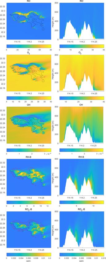
3532                   Y. Wang et al.: The impact of inhomogeneous emissions and topography on ozone photochemistry

of global models and 1–50 km in the case of regional mod-          et al. (2016) investigated the sensitivity of the segregation of
els used for operational numerical weather and climate pre-        volatile organic compounds (VOCs) to weather conditions
dictions. Thus, in both cases, small-scale processes such as       (e.g., temperature, humidity, and the presence of clouds).
turbulent motions in the boundary layer, mountain flows, sea       They showed that isoprene segregation is largest under warm
breeze, urban dynamics, and shallow clouds, as well as the         and convective conditions. Kim et al. (2016) showed that
complexity of surface chemical emissions, are crudely rep-         the segregation intensity of isoprene and OH differs at low-
resented or parameterized. Coarse models, for example, as-         and high-nitrogen-oxide (NOx ) levels caused by the primary
sume total mixing between trace species inside each grid           production and loss reactions of OH under a different NOx
mesh and therefore do not accurately account for the seg-          regime. Li et al. (2017) added the effect of aqueous-phase
regation that may exist between these species in turbulent         chemistry in a LES model and showed that the segregation of
flows. The segregation effect is important for fast reactions,     OH and isoprene is enhanced in clouds. Studies focusing on
of which the chemical timescale is shorter than the tur-           isoprene chemistry in a forested region have been initiated to
bulent timescale. In this case the reactants remain segre-         understand the underestimation of the OH in global models
gated rather than reacting, and such segregation tends to re-      (Dlugi et al., 2019; Ouwersloot et al., 2011). These studies all
duce the averaged rate at which chemical reactions happen          used flat domains and calculated the domain-averaged segre-
within a model grid mesh (Komori et al., 1991; Schumann,           gation intensities to account for the errors induced by the tur-
1989). Previous studies, such as Vilà-Guerau de Arellano and       bulence in regional or global models. However, the impact of
Duynkerke (1993) and Kramm and Meixner (2000), consid-             the terrain on the segregation was not considered. Previous
ered the segregation effect in the boundary layer parameter-       studies showed that complex terrain has an important impact
ization in the chemical transport models and showed that it        on the turbulence structure in the boundary layer (e.g., Cao et
is important to take the segregation into account in current       al., 2012; Rotach et al., 2015; Liang et al., 2020) and on the
photochemical models.                                              evolution with time of the boundary layer height (De Wekker
   Numerical treatment of the turbulent flow can be provided       and Kossmann, 2015). Therefore, the segregation intensity is
by large-eddy simulation (LES) models. LES is a rapidly            expected to be affected by the topography.
evolving approach for modeling the turbulent flows, which             This paper uses a LES model included in the Weather
was initially proposed by Smagorinsky (1963) and first ex-         Research and Forecasting (WRF) model (Skamarock et al.,
plored by Deardorff (1970). In this approach, the unsteady         2008, 2019) to investigate the importance of segregation be-
Navier–Stokes and continuity equations are filtered to re-         tween reacting species in an area where surface emissions are
move the smallest eddies while capturing the eddy motions at       spatially very inhomogeneous and the flow is turbulent un-
a size larger than a specified cutoff width. The interactions of   der the influence of a complex topography. Under such con-
the larger, resolved eddies and the smaller, unresolved eddies     ditions, the vertical mixing and the reaction rates between
are addressed by specifying a SGS stress model (Deardorff,         chemical species in the boundary layer are expected to be
1970; Smagorinsky, 1963).                                          sensitive to the strength of the large eddies. The simulations
   The LES technique has been used in past studies to              are performed in a geographical area covering Hong Kong
quantify the segregation effect in the turbulent atmospheric       Island. The surface wind measurements from the Hong Kong
boundary layer. Schumann (1989) simulated a single reaction        Observatory (HKO) station show the prevailing wind blow-
in the convective boundary layer with one bottom-up and one        ing from the east about 80 % of the time and from the west
top-down tracer and showed that the segregation of one reac-       about 15 % of the time (Shu et al., 2015). There are two im-
tion is dependent on the ratio of the chemical and turbulent       portant features in the air pollution in Hong Kong: the pol-
timescales, the concentration ratio of the two reactants, and      lution sources are concentrated in the very dense urban re-
the initial condition. Patton et al. (2001) used LES to simu-      gion, mostly along the coast, while natural emissions occur
late scalars that are emitted from forest canopy with different    in large forested areas in the center of the island; both regions
decay rates and presented the influence of chemical reactivity     are separated by complex topography. With the intense and
on the scalar distribution, variance, and vertical flux, which     inhomogeneous emissions in such an urban environment, the
affect the segregation. Other LES studies with different con-      resultant segregation can cause a large impact on the calcu-
figurations of surface emissions pointed out that spatially in-    lation of chemical reactions (Li et al., 2021). This impact is
homogeneous emissions influence the segregation intensities        expected to be even larger with the influence of complex to-
considerably. These studies, such as Krol et al. (2000), Auger     pography. In this study, we therefore set up a domain with
and Legras (2007), and Ouwersloot et al. (2011), mainly fo-        a mountainous terrain characterized by complex flows deter-
cused on isoprene chemistry and compared the segregation           mined by the topography and the occurrence of related tur-
intensities of the reaction between isoprene and the hydroxyl      bulent motions.
radical (OH) with homogenous and inhomogeneous isoprene               The purpose of the study is to investigate the importance
emissions and showed that the heterogeneity in the emissions       of interactions between chemistry and turbulence in the plan-
largely increases the segregation intensities. There are other     etary boundary layer (PBL) as well as to assess how the spa-
factors that affect the segregation intensities. For example, Li   tial segregation between chemical species affects the nonlin-

Atmos. Chem. Phys., 21, 3531–3553, 2021                                              https://doi.org/10.5194/acp-21-3531-2021

Y. Wang et al.: The impact of inhomogeneous emissions and topography on ozone photochemistry                               3533

ear production and destruction rates of key chemical species      100 m. The vertical layers were the same for both domains
including ozone. Since the study is intended to be concep-        with 100 vertical levels, and the model top was set at 4 km
tual, we adopt a simple chemical scheme to represent the          altitude. Double periodic boundary conditions were used in
chemical interactions between ozone and its precursors. We        both the west–east and south–north directions for the outer
make plausible assumptions about the spatial distribution         domain. One-way nesting was used, in which the outer do-
of the surface emissions of primary species emitted in the        main provided turbulence-inclusive boundary conditions for
forested and urbanized areas of the island. We estimate how       the inner domain (Moeng et al., 2007; Muñoz-Esparza et al.,
the vertical eddy transport fluxes of the chemical species and    2014).
the covariance between their concentrations, generally unac-         The initial profiles for the potential temperature (θ ) and
counted for in coarse atmospheric models, affect the distri-      water mixing ratio (q) for the outer domain were taken from
bution of chemical species in the lowest levels of the atmo-      the output of the mesoscale WRF run operated at a spa-
sphere in the vicinity of the island.                             tial resolution of 1.33 km (shown by the dashed green line
   The present modeling study should be viewed as a step to-      in Fig. 1) and were interpolated to 40 m vertical grid spac-
wards a more complex and realistic investigation of chemical      ing, with the highest level located at 4 km. The date (1 Au-
and turbulent processes occurring in the densely populated        gust 2018) and time of the day (04:00 UTC; 12:00 local time)
urban area of Hong Kong, characterized by a complex urban         were chosen to correspond to a typical summer condition
canopy of high-rise buildings and street canyons built on an      in Hong Kong with a well-developed convective boundary
uneven topography surrounded by the ocean and affected by         layer. Four cases were considered, with initial winds blowing
emissions in mainland China and other Asian countries and         uniformly from the west (TERW; TER stands for terrain), the
by the presence of an active harbor with intense shipping in      east (TERE), the south (TERS), and the north (TERN), re-
the region. The present study focuses on the impact of the        spectively. The initial wind speed in each case was equal to
heterogenous emissions and the turbulent flow generated by        10 m s−1 .
the topography on chemical processes. The model descrip-             The LES version adopted here used Deardorff’s turbulent
tion and dynamical and chemical settings are introduced in        kinetic energy (TKE) scheme to compute the SGS eddy vis-
Sect. 2. Results of the large-eddy simulations and the inter-     cosity and eddy diffusivity for turbulent mixing. The Coriolis
pretations of the model output are presented in Sect. 3. Sec-     parameter was set according to the latitude of Hong Kong Is-
tion 4 provides the principal conclusions of this study.          land. The Kessler microphysics scheme (Kessler, 1969) was
                                                                  used to derive cloudiness in the model. The WRF’s radia-
                                                                  tion, land surface, and PBL schemes were all turned off. We
2     Methodology                                                 applied a fixed sensible heat flux of 230 W m−2 at the bot-
                                                                  tom boundary, while the latent heat flux was calculated in the
2.1    Model description
                                                                  model from the surface water vapor content specified at the
The WRF model (version 4.0.2) with the ARW (Advanced              beginning of the simulations. We chose to apply a relatively
Research WRF) core (Skamarock et al., 2008, 2019) was             small sensible heat flux (compared to summer noon condi-
used to perform mesoscale meteorology simulations that pro-       tions in Hong Kong) in order to produce a gradual devel-
vided the initial fields for the large-eddy simulations. The      opment of the boundary layer and keep the convection con-
LES module included in WRF was run in an idealized mode           dition unchanged during the course of the simulation. With
as implemented and evaluated by Moeng et al. (2007), Kirkil       this choice, the buoyancy flux was dominated in the simula-
et al. (2012), and Yamaguchi and Feingold (2012). A low-          tion by the kinematic sensible heat flux, which is about 2–3
pass filter was applied to separate the large and small ed-       times larger than the kinematic moisture heat flux.
dies, where the large eddies (energy-injection scales near the       The outer model domain was assumed to be entirely flat,
classic inertial range of 3D turbulence) were explicitly re-      while the inner domain included a representation of the to-
solved, while the small eddies were parameterized by the          pography of Hong Kong Island. This modeling setup fol-
SGS model. In the idealized LES, the initial physical con-        lowed the approach of Kosović et al. (2014). The eleva-
ditions were specified by uniform values over the entire do-      tion of the surface was taken from the ALOS world 3D
main; a random perturbation was imposed initially on the          data (Takaku et al., 2014), distributed by OpenTopography
mean temperature field at the lowest four grid levels to initi-   (https://opentopography.org; last access: 1 June 2020), with
ate the turbulent motions.                                        a spatial resolution of 30 m. To avoid numerical errors due to
                                                                  the terrain-following coordinate, the terrain was somewhat
2.2    Dynamical settings                                         smoothed in areas where the surface slope exceeds 25◦ . The
                                                                  smoothed terrain height is shown in Fig. 2a. To simplify the
A nested two-domain setup was adopted for the LES simu-           simulation, and to focus on the terrain shape instead of the
lation. The size of the outer domain was 45 km × 45 km, and       terrain types, the surface of the entire domain was set as land
the spatial resolution was 300 m. The size of the inner do-       to ignore the influence of the sea.
main was 24 km × 24 km, with a horizontal grid spacing of

https://doi.org/10.5194/acp-21-3531-2021                                           Atmos. Chem. Phys., 21, 3531–3553, 2021
3534                   Y. Wang et al.: The impact of inhomogeneous emissions and topography on ozone photochemistry

Figure 1. The evolution of the profiles for potential temperature (a) and water mixing ratio (b) from mesoscale WRF (dashed green lines
at 04:00 UTC; dashed magenta lines at 05:00 UTC) and LES (solid red lines for hour 2 from the start time; solid blue lines for hour 4).
The measurements at King’s Park station taken at 05:00 UTC are shown by black lines (data source: http://www.hko.gov.hk, last access:
13 January 2020).

Figure 2. Elevation of the topography for Hong Kong Island (a) and emission map (b); red is the anthropogenic emission area, and green
represents the biogenic emission.

2.3    Chemical settings                                              beled -B) VOCs, respectively. RH-A was treated as a sur-
                                                                      rogate for propane and RH-B as a surrogate for isoprene.
                                                                      The corresponding rate constants (k) for the oxidation by
A simple O3 –NOx –VOC chemical mechanism with 15 re-
                                                                      the hydroxyl radical OH at a temperature of 300 K are equal
active species and 18 photochemical reactions (see Table 1)
                                                                      to 1.1 × 10⁻¹² and 1.0 × 10⁻¹⁰ cm3 molec.−1 s−1 , respec-
was adopted in this conceptual study and is based on the sim-
                                                                      tively. We can derive the lifetime of RH-A and RH-B by
ple scheme for ozone production from hydrocarbon oxida-
                                                                      the expression 1/ (k × [OH]), with the respective values of
tion described in the textbook by Brasseur and Jacob (2017).
                                                                      the rate constants k. With an OH concentration ([OH]) of
We included two primary hydrocarbons, RH-A and RH-B,
                                                                      5 × 10⁶ molec. cm−3 , the corresponding chemical lifetimes
which represent anthropogenic (labeled -A) and biogenic (la-

Atmos. Chem. Phys., 21, 3531–3553, 2021                                                 https://doi.org/10.5194/acp-21-3531-2021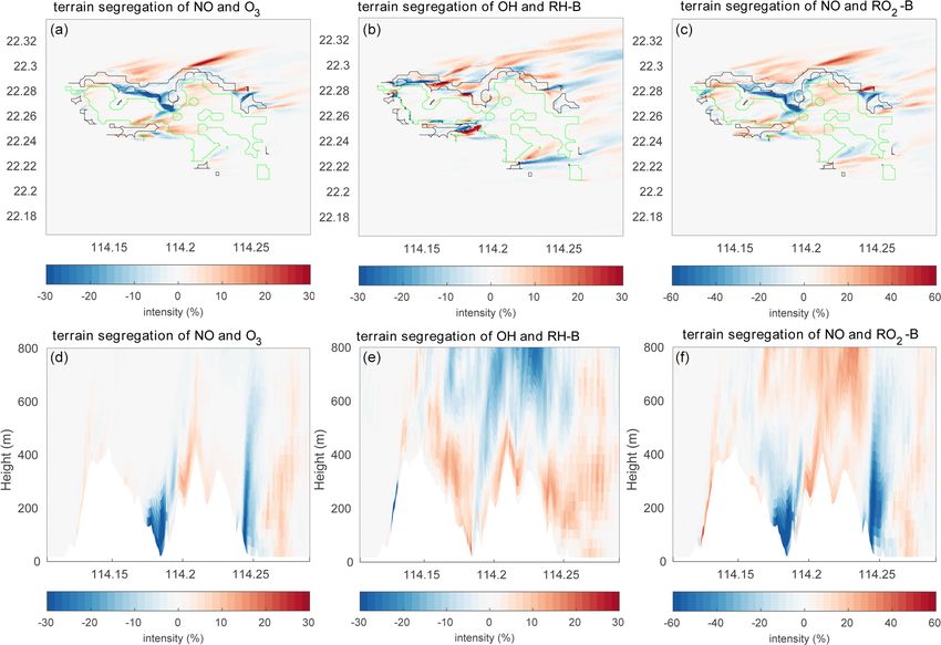
Y. Wang et al.: The impact of inhomogeneous emissions and topography on ozone photochemistry                                     3535

of RH-A and RH-B are approximately 2 d and 30 min, re-             The detailed deposition velocities for the different species
spectively.                                                        and the different land types are provided in Table 3.
   Among all the species, NO, CO, RH-A, and RH-B were                 In order to generate reasonable initial profiles for the
emitted at the surface. The background conditions of the           chemical species for the two-domain simulations and to re-
polluted atmosphere were represented by assuming emis-             duce the spin-up time, a simple one-domain LES simula-
sion rates in the outer domain to be uniform, with values of       tion was run for 2 d using the same chemical scheme as in
1.2 × 10¹² , 8.0 × 10¹² , and 7.0 × 10¹¹ molec. cm−2 s−1 , for     the two-domain simulation. The one-domain LES used the
NO, CO, and RH-A respectively. The RH-B emission was               same homogeneous emissions as described above. The time-
set to be 3.0 × 10¹¹ molec. cm−2 s−1 for the conditions in         varying photolysis rates were calculated by the TUV (tropo-
Hong Kong with a large tropical forested area. For the in-         spheric ultraviolet and visible) scheme for producing the di-
ner domain, we considered two specific regions correspond-         urnal variation in the photochemistry. The domain-averaged
ing to urban and forested areas, based on information pro-         profiles for the chemical species at 12:00 local time of the
vided by the land use map from ESA CCI (ESA, 2017;                 second day were then used as the chemical initial profiles for
https://www.esa-landcover-cci.org, last access: 1 June 2020).      the two-domain simulations. The initial profiles are shown
The resulting emission map on the nested domain that in-           by green lines in Fig. 3.
cludes terrain features is shown in Fig. 2b, with NO, CO, and
RH-A emitted in the urban region and RH-B emitted in the           2.4   Formulations of chemistry–turbulence interactions
forested region. The emission rates in the inner domain were
calculated by dividing the corresponding values adopted in         Following the concept of the Reynolds decomposition, any
the outer domain by the area fraction of the corresponding         physical variable A, such as the concentration of chemical
land use type, so that the averaged emission rates for the         species, can be expressed as the sum between its mean value
whole inner domain were the same as those of the outer do-         hAi (here hi stands for time average) and the fluctuation A0
main. In order to separate the influence of the emissions and      caused, for example, by turbulent motions:
topography, two additional simulations were conducted. A
                                                                   A = hAi + A0 .                                                 (1)
simulation with homogeneous emissions and without topog-
raphy for both domains (HOMF; HOM stands for homoge-               For a second-order chemical reaction,
neous emission; F stands for flat terrain) was performed as
a baseline experiment. To assess the role of the inhomoge-         A + B → C,                                                     (2)
neous emissions in our results, a simulation with flat terrain
but with inhomogeneous emissions as shown in Fig. 2b (re-          with the reaction rate constant,
ferred to as HETF; HET stands for heterogeneous emission;                    T0
F stands for flat terrain) was also conducted. The details of      k = k0 e − T ,                                                 (3)
all the experiments are listed in Table 2.
   An atmospheric destruction of reservoir species (HNO3 ,         where k0 and T0 are reaction-dependent constants, and the
H2 O2 , ROOH-A, ROOH-B) was applied to balance the sur-            rate R of the reaction is expressed as
face emissions of the primary species. The removal of these
reservoirs by photolytic processes in the atmosphere is slow       R = k · A · B.                                                 (4)
(more than 2 weeks in the case of HNO3 and several days for
                                                                   If we ignore the temperature fluctuation (i.e., T 0 = 0), the
peroxides), so that most of the loss is due to wet removal or
                                                                   averaged reaction rate is
dry deposition. The model did not consider the possible oc-
currence of convective precipitation as often observed during      R = k · hA · Bi = k · hAi · hBi + k · hA0 · B 0 i = k · hAi
summertime in Hong Kong, and hence no detailed formula-
tion was used for the wet removal in the LES model. How-             · hBi · (1 + IAB ) ,                                         (5)
ever, in order to keep a balance (stationary state) in the back-
                                                                   where hA0 · B 0 i is the chemical covariance between the two
ground concentrations and avoid an accumulation of species
                                                                   reacting chemicals, and IAB is called the segregation inten-
produced from the ongoing emissions, the removal of the
                                                                   sity (Danckwerts, 1952), defined as
soluble species HNO3 , H2 O2 , ROOH-A, and ROOH-B oc-
curred with a first-order rate of 2.5 × 10⁻⁵ s−1 (lifetime of              hA0 · B 0 i
about half a day). This lifetime may be viewed as represent-       IAB =               .                                          (6)
                                                                           hAi · hBi
ing the mean time period separating successive convective
rain events during summertime. For the dry deposition on           The intensity of the segregation is therefore equal to the co-
the surface, for the grass/forested areas outside the urban-       variance of the two reactants divided by the product of their
ized regions we adopted values based on the measurements           mean concentrations. IAB is equal to zero when the chemi-
of Wu et al. (2011) and on the analysis of Ganzeveld and           cals A and B are fully mixed and equal to −100 % when the
Lelieveld (1995). The values were reduced over urban areas.        two chemicals are fully segregated. For initially segregated

https://doi.org/10.5194/acp-21-3531-2021                                              Atmos. Chem. Phys., 21, 3531–3553, 2021
3536                         Y. Wang et al.: The impact of inhomogeneous emissions and topography on ozone photochemistry

Table 1. The chemical reactions used in the model. The unit of first-order reaction rate coefficients is per second (s−1 ) and that of second-
order reaction rate coefficients is cubic centimeters per molecule per second (cm3 molec.−1 s−1 ).

       No      Reactions                                                         Reaction rates
       R1      NO2 + hv → NO + O3                                                5.0 × 10⁻³
       R2      O3 + hv → O(1 D) + REST                                           2.5 × 10⁻⁵
       R3      HCHO + hv → HO2 + CO + REST                                       2.5 × 10⁻⁵
       R4      HNO3 + hv → NO2 + OH                                              3.0 × 10⁻⁷
       R5      O(1 D) + M → O3 + REST                                            0.78084 × 1.8 × 10−11 × e110/T + 0.20946 × 3.2 × 10−11 × e70/T ;
       R6      O(1 D) + H2 O → OH + OH                                           2.2 × 10⁻¹⁰
       R7      HO2 + NO → NO2 + OH                                               3.7 × 10⁻¹² × e240.0/T
       R8      O3 + NO → NO2 + REST                                              3.0 × 10⁻¹² × e−1500.0/T
       R9      HO2 + HO2 →H2 O2 + REST                                           2.2 × 10⁻¹³ × e600/T + 1.9 × 10⁻³³ × CM × e980/T
       R10     HO2 + HO2 + H2 O → H2 O2 + REST                                   3.08 × 10⁻³⁴ × e2800/T + 2.66 × 10−54 × CM × e3180/T
       R11     OH + NO2 → HNO3                                                   TROE
       R12     CO + OH → HO2 + REST                                              1.5 × 10−13 × (1 + 2.439 × 10⁻²⁰ × CM )
       R13     HCHO + OH → HO2 + CO + REST                                       5.5 × 10⁻¹² × e125.0/T
       R14     OH + O3 →HO2 + REST                                               1.7 × 10⁻¹² × e−940.0/T
       R15     HO2 + O3 →OH + REST                                               1.0 × 10⁻¹⁴ × e−490.0/T
       R16     RH-A + OH → RO2 -A + REST                                         1.0 × 10⁻¹¹ × e−665.0/T
       R17     RO2 -A + NO → HCHO + HO2 + NO2 + REST                             2.8 × 10⁻¹² × e300.0/T
       R18     RO2 -A + HO2 →ROOH-A + REST                                       4.1 × 10⁻¹³ × e750.0/T
       R19     RH-B + OH → RO2 -B + REST                                         1.0 × 10⁻¹⁰
       R20     RO2 -B + NO → HCHO + HO2 + NO2 + REST                             1.0 × 10⁻¹¹
       R21     RO2 -B + HO2 → ROOH-B + REST                                      1.5 × 10⁻¹¹
    Note that T stands for temperature, M stands for air, CM stands for the air density, and REST stands for the products that are not evaluated.
                                             2
    TROE = k1 /(1.0 + k2 ) × 0.6(1.0/(1.0+log (k2 ))) , k1 = 2.6 × 10−30 × (300/T )3.2 × CM , k2 = k1 /(2.4 × 10−11 × (300/T )1.3 ).

                                                                                            A and B, the corresponding segregation intensity is closer
Table 2. List of the numerical experiments.                                                 to −100 % if the chemical reaction between the two species
                                                                                            is fast. IAB is positive when the concentrations of the two
   Case        With         With                   Winds                                    chemicals are correlated.
   name        terrain      heterogeneous          (m s−1 )                                    The intensity of segregation between two species A and B
                            emissions                                                       is related to the Damköhler number (Da) (Damköhler, 1940):
   HOMF        no           no                     West (u = 10, v = 0)                                     τturb
                                                                                            DaA(B) =               ,                                 (7)
   HETF        no           yes                    West (u = 10, v = 0)                                 τchem,A(B)
   TERW        yes          yes                    West (u = 10, v = 0)
   TERE        yes          yes                    East (u = -10, v = 0)                    where τturb is the turbulent timescale (typically 10 min dur-
   TERS        yes          yes                    South (u = 0, v = 10)                    ing daytime, considerably longer during nighttime), and
   TERN        yes          yes                    North (u = 0, v = -10)                   τchem, A(B) is the reaction timescale of A when reacting with
                                                                                            B. If the chemical timescale of A is shorter than the turbulent
                                                                                            timescale (Da > 1; called the fast chemistry limit), the reac-
                                                                                            tion between A and B is limited by the rate at which turbu-
                                                                                            lent motions bring reacting species together; the covariance
Table 3. Dry deposition velocity used in this study.                                        between fluctuating components as well as the segregation
                                                                                            intensity are high. This occurs when the reaction rate con-
             Chemical             No terrain       With terrain                             stant k is large (Schumann, 1989; Vinuesa and Vilà-Guerau
             compounds             (cm s−1 )        (cm s−1 )                               de Arellano, 2005, 2011) or when the emission of A or B
                                                  forest      other                         is intense (Molemaker and Vilà-Guerau de Arellano, 1998;
                                                                                            Kim et al., 2016; Li et al., 2021). Other factors such as inho-
             O3                         0.06         0.6       0.01
             NO2                        0.04         0.4       0.01
                                                                                            mogeneous emissions (Ouwersloot et al., 2011; Auger and
             HNO3                        0.5           5        0.7                         Legras, 2007; Li et al., 2021) and other structures that ob-
                                                                                            scure mixing also result in a more negative segregation in-
                                                                                            tensity. Under this situation, coarse models such as regional

Atmos. Chem. Phys., 21, 3531–3553, 2021                                                                             https://doi.org/10.5194/acp-21-3531-2021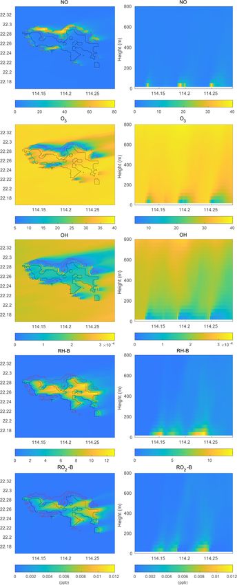
Y. Wang et al.: The impact of inhomogeneous emissions and topography on ozone photochemistry                                           3537

Figure 3. Domain-averaged profiles of the selected chemical compounds at the initial time (green lines), hour 2 (red lines), and hour 4 (blue
lines) for the HOMF case.

chemical transport models may not provide accurate results               tions, represented, for example, by the concentration aver-
since they ignore the influence of subgrid-scale turbulence on           aged over a grid cell in a global and regional model. The sec-
the rate at which a reaction between A and B occurs. When                ond term accounts for the contribution of subgrid chemical–
the Damköhler number Da  1 (called the slow chemistry                   turbulent interactions and can be estimated using a large-
limit), the chemical species A under consideration is well               eddy simulation. The effective rate constant keff of a reac-
mixed with small covariances with reactant B and with no                 tion affected by turbulent motions is therefore (Vinuesa and
significant segregation. In this case, the reaction is controlled        Vilà-Guerau De Arellano, 2005)
by chemistry, and its rate is proportional to the product of the
                                                                         keff = k(1 + IAB ).                                             (8)
mean concentrations. This represents a case in which the rate
of chemical reactions is well represented in coarse models.              Thus, a negative value of the segregation intensity IAB tends
When the Damköhler number is close to 1, the interaction                 to reduce the average rate at which a reaction occurs, while a
between chemistry and turbulence is strong as the chemical               positive value of IAB leads to an enhancement in this rate.
species are equally controlled by chemistry and turbulence.                 The segregation intensity can also be written as a func-
   In the Reynolds decomposition described here, the reac-               tion of the correlation coefficient and the concentration fluc-
tion rate is thus expressed by the sum of two terms: the first           tuation intensity, as shown in the paper by Ouwersloot et
term is proportional to the product of the mean concentra-               al. (2011). The standard deviation of A is expressed as σA =

https://doi.org/10.5194/acp-21-3531-2021                                                   Atmos. Chem. Phys., 21, 3531–3553, 2021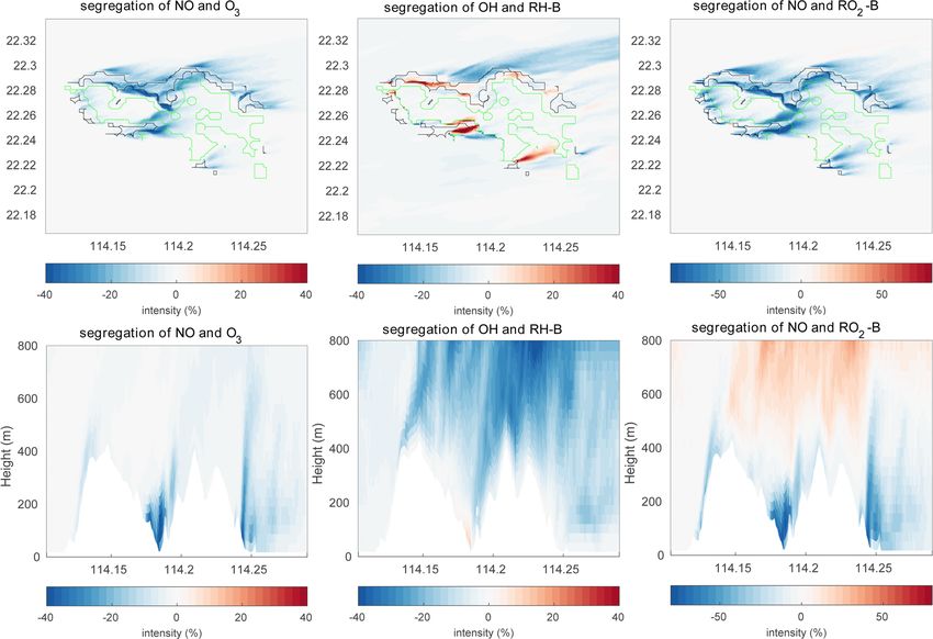
3538                   Y. Wang et al.: The impact of inhomogeneous emissions and topography on ozone photochemistry
          1
hA0 · A0 i 2 , and the covariance of A and B is σAB = hA0 · B 0 i,   the South China Sea. The red and blue solid lines show
so the segregation intensity becomes                                 the large-eddy simulation (HOMF) after 2 and 4 integration
                                                                     hours, respectively. The simulated water vapor from LES
          σAB     σA σB
IAB =           ·   ·    = r · iA · iB ,                      (9)    is higher than in the mesoscale model, and the agreement
         σA · σB hAi hBi                                             with the measurements is improved, especially at high alti-
where                                                                tudes. The convective boundary layer height is detected by
                                                                     the virtual potential temperature (θv ) gradient method, which
       σAB                                                                                                    θv (z)−θvs
r=                                                           (10)    is defined as the height where ∂θ    v
                                                                                                        ∂z =     z−zs    (the subscript
      σA · σB                                                        “s” represents the surface) first exceeds a threshold value
is the correlation coefficient of A and B, which determines          (Liu and Liang, 2010). Due to the constant surface heat flux
the sign of the segregation intensity, while                         forcing, the PBL height gradually increases with a trend of
                                                                     ∼ 0.028 m s−1 . The PBL height is about 797 and 985 m at
       σA           σB                                               hour 2 and hour 4, respectively. This deepening tendency of
iA =       and iB =     ,                                    (11)
       hAi          hBi                                              the PBL is the same as in the mesoscale WRF simulation,
                                                                     but the growth in the PBL height in LES is slower than that
defined as the concentration fluctuation intensity of A and          in WRF because of the small surface heat flux adopted in the
B, controls the strength of the segregation. In this paper, the      LES model. It should be noted that the derived PBL heights
mean fields of the chemical species were all calculated as a         are sensitive to the estimation methods (e.g., Seidel et al.,
1 h time average at given points in the domain.                      2010; Li et al., 2019). The virtual potential temperature gra-
                                                                     dient method is chosen because the calculated PBL height
3     Results                                                        is consistent with that derived in the mesoscale WRF. How-
                                                                     ever, to be considered as realistic, the calculated PBL heights
The simulations for the inner domain were analyzed and               should be compared to a sufficient number of observations
are shown in this section. The results of the simulations are        rather than mesoscale WRF estimates. In fact, the PBL pro-
presented in several subsections. First, we derive domain-           cesses and cloud convection are difficult to be represented
averaged characteristics of physical and chemical quanti-            in the mesoscale models (Mapes et al., 2004; Barth et al.,
ties (i.e., temperature, humidity, concentrations of chemical        2007), and the derived PBL heights are strongly affected by
species) from a baseline experiment (HOMF) that ran with             the cloud physics and PBL schemes adopted in the simula-
uniform surface emissions in the absence of topography. Sec-         tions (e.g., Li et al., 2019). The estimated turbulent timescale
ond, we analyze the effects of inhomogeneous (spatially con-         for the LES simulation is about 9 min, which is similar to
centrated) surface emissions (HETF) on the distribution of           timescales reported in previous studies (e.g., Anfossi et al.,
chemical species and on the spatial segregation between re-          2006).
acting species. Third, we discuss the impact of the topogra-            Figure 3 shows the domain-mean profiles of several chem-
phy on the same quantities. Finally, we assess the influence         ical species at hours 2 and 4. The green lines represent the
of different mean wind directions on our model results.              initial profiles applied in the LES model. The profiles at
                                                                     hours 2 and 4 are very similar, which suggests that station-
3.1    General development                                           ary conditions have been reached in the LES simulation. The
                                                                     atmospheric concentrations of the species emitted at the sur-
The time evolution of the profiles of the potential tempera-         face (NO, RH-A, RH-B) are largest near the ground and de-
ture and water vapor mixing ratio (averaged over the entire          crease with altitude. Because O3 is consumed by NO and
domain) is shown in Fig. 1. The dashed lines represent the           since NO is highest at the surface, the O3 concentration is
output from the mesoscale WRF model at a spatial resolution          lowest in the bottom layers of the model. The same situation
of 1.33 km. The dashed green lines at 04:00 UTC (12:00 local         exists for OH that reacts with the primary species CO, RH-
time) represent the initial profiles adopted for the LES simu-       A, and RH-B that are emitted at the surface. NO2 is produced
lation, and the dashed magenta lines are the WRF output at           by the reaction between NO and O3 ; this reaction is therefore
05:00 UTC (13:00 local time). At this time, the temperature          largely dependent on the NO concentration, so that the NO2
has increased in the boundary layer, and the top of the PBL          shows a similar profile to that of NO. RO2 -A and RO2 -B are
has been lifted in response to the warming of the surface. The       produced by the oxidation by OH of RH-A and RH-B; how-
sounding measurements at 05:00 UTC at King’s Park station            ever, RH-A reacts more slowly than RH-B, and therefore the
are used to validate the simulated physical quantities (black        RO2 -A vertical profile is more affected by the concentration
lines in Fig. 1). The mesoscale WRF model reproduces the             of OH than RO2 -B that shares the same structure as that of
potential temperature quite well, while it underestimates the        RH-B.
water vapor mixing ratio, especially in the boundary layer.             In order to assess the average effect of turbulence on the
This may be related to a simulated weaker southerly wind,            reaction rates, we calculated the segregation intensities (IAB )
which results in relatively less water vapor transport from

Atmos. Chem. Phys., 21, 3531–3553, 2021                                                https://doi.org/10.5194/acp-21-3531-2021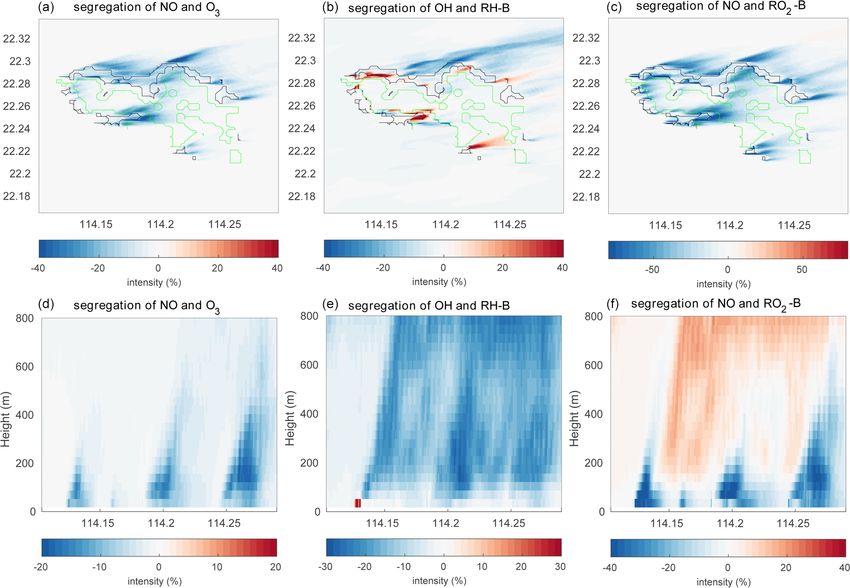
Y. Wang et al.: The impact of inhomogeneous emissions and topography on ozone photochemistry                                          3539

Figure 4. Domain-averaged segregation intensity profiles of selected reactions at hour 2 (red) and hour 4 (blue) for the HOMF case.

using Eq. (6) and averaged them over the entire domain                  the weather conditions and the concentration of the species
(shown in Fig. 4) for the following five reactions:                     (Li et al., 2016). As a result, the calculated values of Da can
                                                                        vary over a wide range and change as one adopts a different
NO + O3 → NO2 + O2                                           (R8)       chemical mechanism. The horizontal averaged segregation
RH-A + OH → RO2 -A                                          (R16)       profiles for the selected reactions from the surface to 1000 m
RO2 -A + NO → HCHO + HO2 + NO2                              (R17)       are shown in Fig. 4. For the LES experiment with flat terrain
                                                                        and homogenous emissions, the segregation is weak near the
RH-B + OH → RO2 -B                                          (R19)
                                                                        surface and becomes larger at higher altitudes. It is gener-
RO2 -B + NO → HCHO + HO2 + NO2 .                            (R20)       ated by the turbulent patterns of the flow. The segregation
   Among these reactions, Reaction (R8) plays a key role                intensities for Reactions (R8), (R16), (R17), and (R19) are
in linking the atmospheric levels of tropospheric ozone                 negative, which highlights the anti-correlation between the
and nitrogen oxides; Reactions (R16) and (R17) represent                atmospheric concentration of the reactants. The segregation
the degradation path of anthropogenic VOCs, while Reac-                 intensity, however, is positive in the case of Reaction (R20)
tions (R19) and (R20) account for the same reactions but for            because RO2 and NO are positively correlated. We calculated
biogenic VOCs. In this study, we only analyze the segrega-              the statistics from the segregation fields for the center region
tion effect in the boundary layer up to 800 m to avoid the              of the domain (14 × 14 km2 ) so that we exclude the influ-
more complex influence from clouds that are formed higher               ence of the buffering zone near the lateral boundaries of the
up in the atmosphere. Using Eq. (7), we derive in the daytime           domain. We provide values for two altitude layers: 0–500 and
boundary layer Damköhler numbers Da(NO) and Da(O3 ) of                  500–800 m, as shown in Table 4. The separation at 500 m is
9.8 and 0.5 respectively for Reaction (R8). The Damköh-                 adopted to make comparisons with subsequent simulations
ler numbers for the degradation of primary anthropogenic                in which the effect of the terrain is considered. The mean
and biogenic hydrocarbons RH-A and RH-B by the hydroxyl                 segregation intensity for the reaction between NO and O3 is
radical OH are 0.004 and 0.3, respectively. This indicates              −0.60 % below 500 m and −0.95 % above 500 m, which are
that the oxidation of the anthropogenic hydrocarbon (surro-             the smallest values among the five selected reactions. This
gate of propane) is slow, while it is considerably faster in            results from the fact that the reaction rate between NO and
the case of the biogenic hydrocarbon (surrogate of isoprene).           O3 is relatively small, as well as the rapid cycling between
The value of 0.3 calculated for RH-B is in the range of 0.01–           NO and NO2 . The intensities for the reaction between the
1.0 derived by previous studies of isoprene (e.g., Patton et            anthropogenic hydrocarbon (RH-A) and OH are −0.84 % at
al., 2001; Vinuesa and Vilà-Guerau de Arellano, 2005; Li et             the lowest levels and −1.52 % at the highest level, respec-
al., 2016; Dlugi et al., 2019). The Damköhler numbers for               tively. The reaction of the biogenic hydrocarbon (RH-B) is
the reaction of peroxy radicals with nitric oxide, Da(RO2 -             considerably faster than that of RH-A; as a result, segrega-
A) and Da(RO2 -B), are equal to 188 and 248 respectively,               tion is as large as −5.08 % and −8.38 % for the low and
which indicates that the reaction of the organic peroxy radi-           high levels, respectively. The calculated segregation inten-
cals with NO is fast for both species from anthropogenic and            sity for RH-B and OH is comparable to the values from pre-
biogenic origins (Verver et al., 2000). The calculation of the          vious studies, e.g., −7 % (PBL-averaged), as reported for the
Damköhler number is sensitive to several factors including              homogeneous case by Ouwersloot et al. (2011), and −5 %

https://doi.org/10.5194/acp-21-3531-2021                                                  Atmos. Chem. Phys., 21, 3531–3553, 2021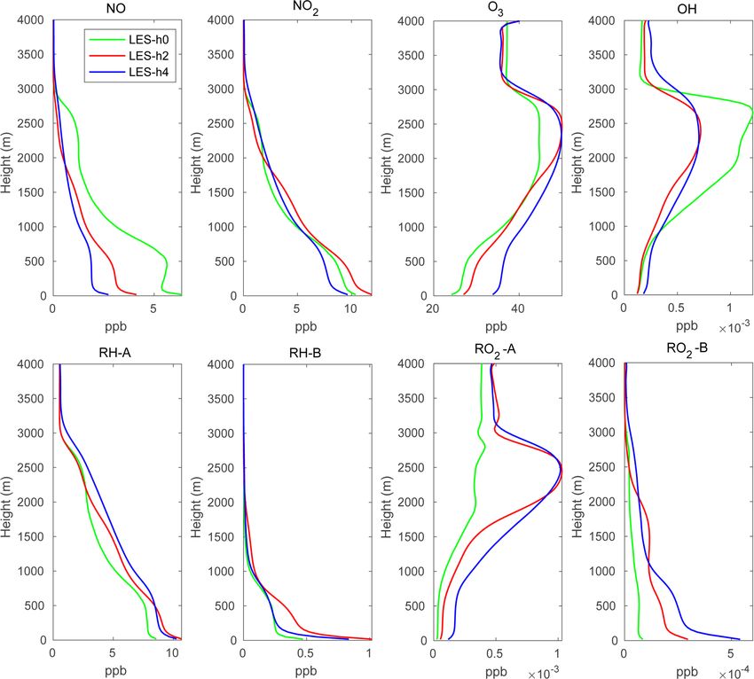
3540 Y. Wang et al.: The impact of inhomogeneous emissions and topography on ozone photochemistry
to −6 %, as found by Kim et al. (2016). Kim et al. (2016)
Table 4. List of the calculated segregation intensities for the center region (14 × 14 km2 ) of the domain.
TERN
TERS
TERE
TERW
HETF
HOMF
name
Case
showed that the segregation intensity between isoprene and
OH varies with NOx levels. This results from the fact that
the primary OH production and loss rates vary according to
500–800
500–800
500–800
500–800
500–800
500–800
Altitude
0–500
0–500
0–500
0–500
0–500
0–500
the NOx regime under consideration. Therefore, the differ-
(m)
ences between values reported by different studies can be
attributed, at least in part, to the different NOx levels. Ouw-
−2.84 ± 2.93 (−32.28 to −0.11)
−1.59 ± 2.62 (−35.05 to −0.15)
−2.78 ± 5.36 (−68.79 to −0.07)
−2.45 ± 3.87 (−30.34 to −0.14)
−3.04 ± 5.77 (−55.84 to −0.06)
−2.40 ± 3.60 (−41.34 to −0.15)
−3.14 ± 6.05 (−59.18 to −0.09)
−2.25 ± 3.35 (−27.39 to −0.16)
−3.21 ± 6.01 (−50.44 to −0.03)
−0.60 ± 0.20 (−1.52 to −0.12)
−0.95 ± 0.29 (−2.70 to −0.25)
ersloot et al. (2011) used a low-NOx condition, while our
−2.83 ± 4.20 (−45.49–0.08)
study considers a polluted situation with high-NOx concen-
trations. In order to further compare with the previous stud-
ies, the relationship between segregation intensity and corre-
lation coefficient (r) for the reaction between RH-B and OH
NO + O3 (R8)
is plotted in Fig. 5. The calculated correlation coefficients
are mostly in the range of −0.6 to −1.0, which is consis-
tent with the model results from Ouwersloot et al. (2011),
while they are larger than the measurements from some cam-
paigns resulting from the measurement noise (Dlugi et al.,
−4.39 ± 3.81 (−29.83 to −0.09)
−2.17 ± 3.18 (−31.34 to −0.06)
−3.41 ± 4.90 (−35.48 to −0.10)
−3.47 ± 4.88 (−37.73 to −0.07)
−3.20 ± 4.43 (−27.49 to −0.10)
−0.84 ± 0.30 (−2.46 to −0.15)
−1.52 ± 0.54 (−4.97 to −0.34)
−3.15 ± 5.47 (−57.74–28.52)
−3.54 ± 6.25 (−53.98–16.75)
−3.61 ± 6.13 (−47.10–15.52)
2019). The mean values calculated for NO and RO2 -A are
−3.76 ± 4.57 (−39.21–8.13)
−3.39 ± 5.77 (−47.98–6.40)
−3.14 % and −5.38 %. For the reaction of the positively cor-
related species, NO and RO2 -B, the segregation intensities
RH-A + OH (R16)
are +2.77 % and +5.43 %.
Figure 4 also shows that the negative segregation intensi-
ties are larger for hour 2 than for hour 4 of the simulation,
while the positive segregation is smaller at hour 2 compared
to hour 4. This highlights the enhanced mixing of the tracers
Segregation intensity (%): mean ± SD (range)
as time proceeds, so that the reactions become increasingly
−5.08 ± 1.82 (−12.5 to −0.50)
−8.38 ± 2.68 (−22.4 to −1.87)
−15.80 ± 11.98 (−63.06–1.38)
−8.50 ± 9.21 (−63.65–119.59)
−6.62 ± 8.26 (−73.19–199.54)
−10.58 ± 10.12 (−67.12–2.75)
−5.86 ± 6.67 (−64.26–188.58)
−7.20 ± 8.21 (−77.13–112.37)
−10.08 ± 9.63 (−57.11–1.16)
−5.01 ± 7.35 (−50.73–93.12)
−11.16 ± 9.46 (−52.18–0.77)
−10.19 ± 8.60 (−50.08–4.14)
effective.
3.2 Impact of inhomogeneous surface emissions on the
RH-B + OH (R19)
chemical reactions
To investigate the impact of the spatially inhomogeneous
emissions on Hong Kong Island, a control run (HETF) was
conducted using the emission distribution shown in Fig. 2.
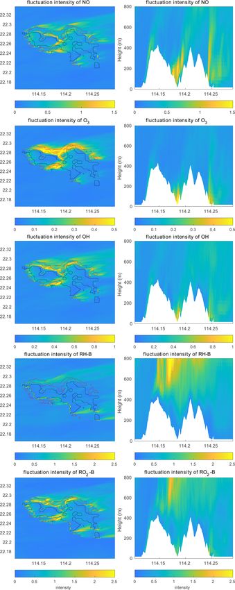
The mean concentrations of several chemical species near
−10.08 ± 10.72 (−88.80 to −0.38)
the surface and in a vertical cross section along the west-
−12.32 ± 8.95 (−63.99 to −0.51)
−9.51 ± 10.97 (−67.80 to −0.78)
−9.07 ± 13.13 (−89.67 to −0.33)
−9.79 ± 10.75 (−72.13 to −0.65)
−9.56 ± 13.78 (−90.40 to −0.38)
−9.79 ± 13.72 (−90.42 to −0.43)
−6.86 ± 7.57 (−65.35 to −0.66)
−9.21 ± 9.98 (−57.32 to −0.69)
−3.14 ± 1.16 (−9.07 to −0.53)
−5.38 ± 1.93 (−17.1 to −1.27)
east direction at latitude 22.275◦ N are shown in Fig. 6. NO
−8.63 ± 12.43 (−95.65–0.10)
with anthropogenic emissions has the highest concentrations
in the urban area at the edge of Hong Kong Island. RH-A
NO + RO2 -A (R17):
shares the same pattern as NO, so it is not shown here. Since
RH-B has a biogenic source located in the forested region
of the island, the highest values are found in the center of
the island. NO2 produced by the reaction between NO and
O3 shows the same pattern as NO, while O3 , which is nega-
tively correlated with NO, exhibits the lowest concentration
in the urbanized area. OH, which is depleted by both anthro-
−5.15 ± 13.95 (−96.73–158.68)
−4.15 ± 12.98 (−98.21–121.93)
−5.60 ± 14.67 (−96.41–108.05)
−2.91 ± 12.38 (−94.63–38.86)
−6.03 ± 13.70 (−95.52–24.90)
5.03 ± 11.18 (−70.11–55.55)
1.65 ± 10.00 (−67.28–57.11)
pogenic and biogenic species, is characterized by low con-
0.90 ± 9.00 (−48.81–32.71)
3.93 ± 7.48 (−50.80–62.30)
1.04 ± 9.05 (−57.58–41.07)
2.77 ± 1.50 (−1.17–9.08)
centrations above the whole island. Since the anthropogenic
5.43 ± 2.33 (0.30–19.0)
emissions including CO and RH-A are considerably larger
NO + RO2 -B (R20)
than the emissions of RH-B, the OH concentrations are low-
est in the urbanized area. The OH concentration also shows
peak values at the edge between the areas dominated by an-
thropogenic and biogenic emissions, where the destruction
of the radical is smallest. The organic peroxy radicals of an-
thropogenic and biogenic origin, RO2 -A and RO2 -B, share
Atmos. Chem. Phys., 21, 3531–3553, 2021 https://doi.org/10.5194/acp-21-3531-2021Y. Wang et al.: The impact of inhomogeneous emissions and topography on ozone photochemistry 3541 Figure 5. Relationship between segregation intensity and correlation coefficient (r) for the reaction between OH and RH-B for (a) the HOMF simulation and (b) the HETF case. the patterns found for OH and RH-B, respectively. This is nous emissions, the correlation coefficients vary between −1 consistent with the discussion in Sect. 3.1. and +0.7, which decide the sign of the segregation intensi- The segregation intensity derived for the HETF case is ties. From the segregation map near the surface, we can see shown in Fig. 7. Since the segregation intensities of the re- that the segregation intensities for NO and RO2 -B are neg- actions of OH with RH-A and NO with RO2 -A have simi- ative, which is different from the HOMF case in which the lar distribution to that of the NO and O3 reaction, they are emissions are homogeneous. In the HOMF simulation, the not shown in the figure. Different from the HOMF experi- emissions of NO and RH-B (which is highly correlated to ment with homogenous emissions, the segregation intensity RO2 -B) are co-located, so NO and RO2 -B are positively cor- from the HETF run is largely dependent on the distribution of related, while in the HETF simulation, the emission of RH-B the emissions. The segregation map near the surface shows is separated from the NO emissions, resulting in a negative that intensity is much larger near the source region than at correlation between NO and RO2 -B. The vertical patterns of other locations. For the reaction of NO and O3 , the concen- the segregation intensity, shown in Fig. 7d–f, indicate that tration distributions of the two species are opposite to each the impact of the emission distribution is substantial from the other, and the segregation effect is negative. Because of the surface to about 500 m height and is affected by the strength stronger depletion of OH by the anthropogenic species (both of convection. It is seen that the segregation for NO and RO2 - CO and RH-A) than by biogenic RH-B, the OH concentra- B is only negative at low altitudes; it becomes positive at tion is lower in the urban region and higher in the forest area, higher levels, where the impact of the separated sources has which results in a opposite pattern to RH-A. Thus, the segre- vanished. This is consistent with what is reported by Ouw- gation effect is negative for the reaction between RH-A and ersloot et al. (2011) and Li et al. (2021) for their cases with OH. This is also the case for the reaction between NO and heterogeneous emissions. The large magnitude of segrega- RO2 -A, since RO2 -A follows the pattern of OH. The seg- tion intensity between RO2 -B and NO near the surface is also regation map for RH-B and OH is complicated, with both comparable to the values reported in Li et al. (2021) in their positive and negative values, depending on the location; the cases with heterogeneous emissions. positive segregation intensities are located mainly at the edge The calculated mean segregation intensities for NO and between urban and forested areas, where OH concentration O3 are −3.21 % and −2.25 % for the low- and high-altitude exhibits some peaks in its concentration. Because RH-B de- bands respectively, which is more than 5 times (low band) pletes OH, the two species are expected to be negatively and 2 times (high band) larger than the HOMF simulation correlated; however, OH is also consumed by other species, with homogeneous emissions (see details in Table 4). Since which affects the distributions of the radical. This implies the influence of the emissions is stronger in the lowest lev- that the heterogenous emissions not only lead to different in- els, the segregation intensity is also larger at lower altitudes. tensity distributions, but they also can change the sign of the In addition to the mean values, the maximum intensity can segregation when one chemical species reacts with several reach −50 %, implying that the impact of the heterogenous species present in different concentrations at separated lo- character of the emissions can be very strong at certain lo- cations. The correlation coefficient for the RH-B and OH is cations, specifically in the vicinity of the source regions. For shown in Fig. 5. Different from the simulation with homoge- the two other negatively correlated reactions, the mean seg- https://doi.org/10.5194/acp-21-3531-2021 Atmos. Chem. Phys., 21, 3531–3553, 2021
3542                     Y. Wang et al.: The impact of inhomogeneous emissions and topography on ozone photochemistry

                                                                          regation intensities for RH-A and OH are −3.61 % (low) and
                                                                          −3.20 % (high), and those for NO and RO2 -A are −9.79 %
                                                                          and −9.21 %. For the reaction of RH-B with OH, which has
                                                                          both positive and negative intensities as shown in Fig. 7,
                                                                          the mean values are −7.20 % and −10.19 %. Even though
                                                                          the total segregation is characterized by a negative intensity,
                                                                          the maximum positive value of this quantity is higher than
                                                                          100 %, which occurs near the surface; this may explain why
                                                                          the negative intensity at low altitudes is smaller than the in-
                                                                          tensity at high altitudes for this reaction. The segregation in-
                                                                          tensities under the inhomogeneous emission conditions are
                                                                          dependent on the distribution of the emission, so that the
                                                                          numbers cannot be compared directly; however, previous
                                                                          studies also show larger segregation intensities with het-
                                                                          erogenous emissions. For instance, Ouwersloot et al. (2011)
                                                                          derive an isoprene segregation intensity of −12.6 % in their
                                                                          heterogeneous case; Kaser et al. (2015) derived intensities as
                                                                          large as −30 % from measurements of isoprene local segre-
                                                                          gation. Regarding the reaction of NO with RO2 -B, the mean
                                                                          segregation intensity at the lower atmospheric levels is neg-
                                                                          ative (−5.15 %) and at higher levels is positive (0.90 %).
                                                                          The small positive value is probably diminished by the nega-
                                                                          tive intensities; therefore, it is smaller when produced in the
                                                                          HOMF simulation with homogeneous surface emissions.

                                                                          3.3   Influence of the complex terrain

                                                                          Over the flat terrain, the PBL evolution is mainly controlled
                                                                          by the upward surface heat flux and by the downward heat
                                                                          flux (entrainment) at the top of the PBL. Over the moun-
                                                                          tains, in addition to the thermally driven forcing, the advec-
                                                                          tion of the flow, the occurrence of mountain waves, and the
                                                                          rotors also play important roles in the turbulence structure
                                                                          (De Wekker and Kossmann, 2015). In order to assess the
                                                                          role of the turbulence generated by the presence of moun-
                                                                          tains in the segregation between chemical species, we now
                                                                          consider the topography of Hong Kong Island in our model
                                                                          simulations (simulation TERW, TERE, TERS, TERN). The
                                                                          terrain is expected to affect the chemical reactions by chang-
                                                                          ing (1) the turbulent strength and (2) the mean distribution of
                                                                          the chemical species. We first show these two effects by con-
                                                                          sidering the simulation TERW, in which the prevailing mean
                                                                          winds are westerlies. The horizontal wind velocity and the
                                                                          total TKE (the sum of resolved TKE and SGS TKE) with the
                                                                          PBL height along latitude 22.275◦ N are displayed in Fig. 8,
                                                                          which shows how the topography affects the wind field and
                                                                          local turbulence. Compared to the case with flat terrain, the
                                                                          wind speed is smaller at the mountain base and in the valley,
                                                                          while it is significantly larger on the top of the mountains.
                                                                          The derived PBL height mirrors the shape of the terrain (De
                                                                          Wekker and Kossmann, 2015). The PBL height is depressed
Figure 6. Volume mixing ratio of the chemical species at the first        above the mountain base due to the subsiding circulation as-
level (left panels) and vertical cross section along latitude 22.275◦ N   sociated with the wind system along the slopes; a significant
(right panels) at hour 4 for the HETF case. The red line shows the        drop in the PBL height is seen over mountain ridges, which
urban area, and the black line shows the forest area.                     is attributed to the Bernoulli effect; and the PBL is elevated

Atmos. Chem. Phys., 21, 3531–3553, 2021                                                     https://doi.org/10.5194/acp-21-3531-2021
Y. Wang et al.: The impact of inhomogeneous emissions and topography on ozone photochemistry 3543 Figure 7. Segregation intensities at the first level (a–c) and the vertical cross section along latitude 22.275◦ N (d–f) at hour 4 for the HETF case. The black line shows the urban area, and the green line shows the forest area. over valleys as the mixed layer is lifted by the horizontal anthropogenic species (CO and RH-A) consume large quan- advection from the high windward terrain and the local up- tities of OH. valley wind system. The TKE mainly increases behind the Figure 10 shows the calculated segregation intensities for steep hills as a result of the flow separation and shear effect three different reactions under consideration in this study. As produced by the slope (Cao et al., 2012). The TKE associated for the mean concentration and the TKE distributions, the with the terrain changes the concentration fluctuations of the structure of the segregation intensities changes with the to- chemical species. pography. For the distributions near the ground, it shares pat- The simulated concentrations of chemical species are terns similar to those found in the HETF case, since the near- shown in Fig. 9. Compared to the concentration distributions surface chemical concentrations are similar in the two model from the HETF case without topography (Fig. 6), the over- experiments. For the vertical structures, the topography not all patterns are similar when represented on quasi-horizontal only lifts the patterns by the height of the terrain, but it also terrain-following surfaces. There are, however, more defined changes the strength of the segregation intensities. For the re- structures in the concentration fields when taking the influ- action between NO and O3 , the calculated mean segregation ence of the terrain into account. For the vertical cross sec- intensity is −3.14 % in the 0–500 m layer and −2.40 % in the tions, since the anthropogenic emissions are located in the 500–800 m layer. These values are similar to those derived in urbanized areas around the mountains, the concentrations of the HETF simulation, implying that the terrain does not sub- NO and ozone are high in the valleys and low over the moun- stantially change the mean segregation. Because of the com- tains. The concentrations of biogenic RH-B are highest near plexity of the topography with a large number of mountain the surface of the mountains since this organic species is ridges and valleys (and hence some possible compensating emitted by the trees located on the slopes of the mountains. effects), the resulting influence of the topography appears on The vertical distribution of OH is low near the surface ev- average to be relatively small. However, the local maximum erywhere above Hong Kong Island because it is depleted by intensity is −59.18 %, which is larger than the −50.44 % ob- both anthropogenic and biogenic species; however, the OH tained in the HETF case. The terrain impact on the reaction concentration is particularly low in the valleys because the of RH-A and OH and NO and RO2 -A is the same as the re- https://doi.org/10.5194/acp-21-3531-2021 Atmos. Chem. Phys., 21, 3531–3553, 2021
You can also read