Novel aerosol extinction coefficients and lidar ratios over the ocean from CALIPSO-CloudSat: evaluation and global statistics
←
→
Page content transcription
If your browser does not render page correctly, please read the page content below
Atmos. Meas. Tech., 12, 2201–2217, 2019
https://doi.org/10.5194/amt-12-2201-2019
© Author(s) 2019. This work is distributed under
the Creative Commons Attribution 4.0 License.

Novel aerosol extinction coefficients and lidar ratios over the ocean
from CALIPSO–CloudSat: evaluation and global statistics
David Painemal1,2 , Marian Clayton1,2 , Richard Ferrare2 , Sharon Burton2 , Damien Josset3 , and Mark Vaughan2
1 ScienceSystems and Applications Inc., Hampton, VA 23666, USA
2 NASA  Langley Research Center, Hampton, VA 23666, USA
3 US Naval Research Laboratory Stennis Space Center, MS 39529, USA

Correspondence: David Painemal (david.painemal@nasa.gov)

Received: 15 October 2018 – Discussion started: 6 November 2018
Revised: 13 March 2019 – Accepted: 20 March 2019 – Published: 10 April 2019

Abstract. Aerosol extinction coefficients (σa ) and lidar ratios   tal aerosol transport offshore. In addition, seasonal transi-
(LRs) are retrieved over the ocean from CALIPSO’s Cloud-           tions associated with biomass burning from June to October
Aerosol Lidar with Orthogonal Polarization (CALIOP) at-            over the southeast Atlantic are well reproduced by CALIOP–
tenuated backscatter profiles by solving the lidar equation        SODA LR.
constrained with aerosol optical depths (AODs) derived by
applying the Synergized Optical Depth of Aerosols (SODA)
algorithm to ocean surface returns measured by CALIOP and
CloudSat’s Cloud Profiling Radar. σa and LR are retrieved          1   Introduction
for two independent scenarios that require somewhat dif-
ferent assumptions: (a) a single homogeneous atmospheric           Advances in our understanding of the 3-D structure of atmo-
layer (1L) for which the LR is constant with height and (b) a      spheric aerosols have been greatly accelerated with the ad-
vertically homogeneous layer with a constant LR overly-            vent of the Cloud-Aerosol Lidar with Orthogonal Polariza-
ing a marine boundary layer with a homogenous LR fixed             tion (CALIOP), on board the Cloud-Aerosol Lidar and In-
at 25 sr (two-layer method, 2L). These new retrievals differ       frared Pathfinder Satellite Observation (CALIPSO; Winker
from the standard CALIPSO version 4.1 (V4) product, as the         et al., 2009, 2010, 2013). CALIOP has provided the first
CALIOP–SODA method does not rely on an aerosol classi-             global view of aerosol distribution in the boundary layer and
fication scheme to select LR. CALIOP–SODA σa and LR                free troposphere (Winker et al., 2013), progressed our knowl-
are evaluated using airborne high-spectral-resolution lidar        edge of the long-range transport of dust (e.g., Liu et al., 2008;
(HSRL) observations over the northwest Atlantic. CALIOP–           Uno et al., 2011; Yu et al., 2015) and smoke (e.g., de Laat et
SODA LR (1L and 2L) positively correlates with its HSRL            al., 2012; Das et al., 2017; Khaykin et al., 2018), and facil-
counterpart (linear correlation coefficient r > 0.67), with a      itated the evaluation of chemical transport models (Nowot-
negative bias smaller than 17.4 % and a good agreement             tnick et al., 2015; Koffi et al., 2016), among many other ac-
for σa (r ≥0.78) with a small negative bias (≤ | − 9.2 %|).        complishments in the area of aerosol and cloud research.
Furthermore, a global comparison of optical depths derived            CALIOP estimates aerosol extinction coefficients on a
by CALIOP–SODA and CALIPSO V4 reveals substantial                  global scale with unprecedented vertical detail. The unde-
discrepancies over regions dominated by dust and smoke             termined problem of solving the lidar equation with two
(0.24), whereas Aqua’s Moderate resolution Imaging Spec-           physical unknowns, the aerosol extinction and backscatter
troradiometer (MODIS) and SODA AOD regional differ-                coefficients, is addressed in the CALIPSO algorithm by re-
ences are within 0.06.                                             lating both variables via an extinction-to-backscatter ratio,
   Global maps of CALIOP–SODA LR feature high values               or lidar ratio (LR). This standard technique (e.g., Fernald,
over littoral zones, consistent with expectations of continen-     1984) expresses the lidar equation in terms of only one un-
                                                                   known, if LR is prescribed. As aerosol types can be related

Published by Copernicus Publications on behalf of the European Geosciences Union.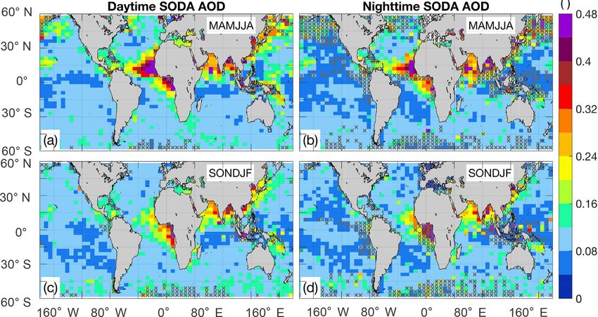
2202                                      D. Painemal et al.: Aerosol extinction coefficients and lidar ratios over the ocean

to specific values of lidar ratios (e.g., Müller et al., 2007),   pects of the CALIPSO Science Team product, as well as for
the CALIPSO algorithm utilizes predefined LR assigned to a        investigating aerosol-related topics in climate research. We
number of aerosol types, which in turn, are identified using      first summarize the algorithm and evaluate the new retrievals
the CALIPSO automated aerosol typing algorithm (Omar et           against state-of-the-art aerosol observations from the NASA
al., 2009; Kim et al., 2018). Thus, the quality of CALIOP re-     Langley airborne High Spectral Resolution Lidar (HSRL,
trievals will depend on how well the actual lidar ratios match    Sects. 3 and 4). Next, we compare the CALIOP–SODA
the pre-tabulated values and to what extent the aerosol typ-      extinction coefficient and AOD with their CALIPSO Sci-
ing algorithm properly classifies aerosols. Another source        ence Team version 4 counterparts. Lastly, we present global
of uncertainty is the detectability limits of the CALIPSO         maps of lidar ratio and marine boundary layer aerosol optical
algorithm, which prevents retrieving aerosol properties for       depth, and provide a physical interpretation for the regional
tenuous aerosol layers (Rogers et al., 2014; Thorsen et al.,      patterns derived from CALIOP–SODA.
2017). For instance, Toth et al. (2018) found that no aerosol
was detected within ∼ 71 % of the CALIOP profiles mea-
sured during daytime and ∼ 41 % of the nighttime measure-         2     Dataset
ments. More aerosol detection during nighttime is explained
                                                                  2.1    CALIOP
by the absence of solar background noise, which leads to a
significantly better signal-to-noise ratio. The aforementioned    Version 4.1 (V4) CALIOP elastic backscatter lidar measure-
factors likely explain discrepancies between CALIOP and           ments at 532 and 1064 nm are utilized in this work. For the
other remote-sensing datasets such as those from the Mod-         derivation of CALIOP–SODA retrievals, we use Level 1 lidar
erate Resolution Imaging Spectroradiometer (MODIS) and            attenuated backscatter and the Level 2 Vertical Feature Mask
AERONET (e.g., Redemann et al., 2012; Schuster et al.,            product, with a 333 m horizontal resolution below 8.2 km.
2012).                                                            CALIOP V4 aerosol extinction coefficients and AOD esti-
   Uncertainty reduction in the selection of LR can be at-        mates are taken from the Level 2 aerosol profile product
tained by constraining the lidar equation solution with an        at 5 km horizontal resolution. To reduce ambiguities in the
independent estimate of aerosol optical depth (AOD). This         CALIOP aerosol classification scheme, we restrict the anal-
implies the minimization of the error between the retrieved       ysis to samples with cloud–aerosol discrimination (CAD)
AOD (estimated from the retrieved extinction coefficient)         scores higher than |50|, equivalent to at least medium con-
and the target AOD by iteratively adjusting LR. Burton et         fidence in the CALIOP layer classification (Liu et al., 2019).
al. (2010) utilize AOD from the MODIS instruments on                 For comparing CALIOP–SODA and V4 products, we fol-
board both Aqua and Terra satellites for estimating aerosol       low the procedure outlined in Koffi et al. (2016): where the
extinction from CALIOP for cases in which AOD ex-                 vertical feature mask (VFM) feature classification flags in-
ceeds 0.15 (0.2) over the ocean (land). Similarly, Royer et       dicate regions of clear air, we set the corresponding extinc-
al. (2010) applied an equivalent method for estimating LR         tion coefficients to zero. While these regions are labeled as
and extinction coefficients over the Po Valley in Italy. Al-      “clear air”, they are simultaneously assumed to be populated
though CALIOP–MODIS retrievals in Burton et al. (2010)            by highly diffuse aerosols that lie well below the CALIOP
tend to compare better with airborne measurements relative        layer detection threshold. Typically, the detection threshold
to the CALIPSO standard product (version 2), MODIS AOD            is range dependent, and varies as a function of molecular
is limited to daytime, and MODIS and CALIOP differ in             density, solar background and other instrument noise, and
their along-track spatial resolution. These previous studies      signal averaging (Vaughan et al., 2009). In terms of AOD,
have proven the value of counting on independent CALIOP           global analysis of CALIOP V3 daytime data by Toth et
retrievals for evaluating CALIPSO’s standard data products.       al. (2018) show that the “aerosol-free” columns reported by
   In this contribution, we present a new method in which         the CALIOP algorithm correspond to a mean MODIS AOD
CALIOP-based lidar ratios and aerosol extinction coeffi-          of 0.03–0.05. A similar analysis by Kim et al. (2017) shows
cients over the nonpolar oceans are obtained by constrain-        that, as expected, CALIPSO extinction and AOD retrieval
ing the retrievals with AOD derived from cross-calibrated         capabilities are substantially better at night than during the
CALIOP and CloudSat Cloud Profiling Radar (CPR) sur-              day. These authors estimate a maximum mean undetected ex-
face echos, using the Synergized Optical Depth of Aerosols        tinction coefficient of ∼ 0.006 km−1 during daytime versus
(SODA) product (Josset et al., 2008). SODA AOD is a suit-         ∼ 0.003 km−1 at night (see their Fig. 5c).
able dataset, as it is collocated with CALIOP by definition
and retrievals are possible during both daytime and night-        2.2    SODA aerosol optical depth
time for the period 2006–2011. After November 2011 SODA
is only available for daytime, as CloudSat has operated in        SODA uses the relationship between CALIOP (532 and
daylight-only operation mode to conserve power (Gravseth          1064 nm) and CPR (3.1 mm, 94 GHz) surface return sig-
and Piepe, 2013). Our goal is to provide an independent           nals, along with a correction for the atmospheric transmis-
CALIOP dataset that can be used for evaluating specific as-       sion at the radar wavelength, to derive AOD at the lidar

Atmos. Meas. Tech., 12, 2201–2217, 2019                                            www.atmos-meas-tech.net/12/2201/2019/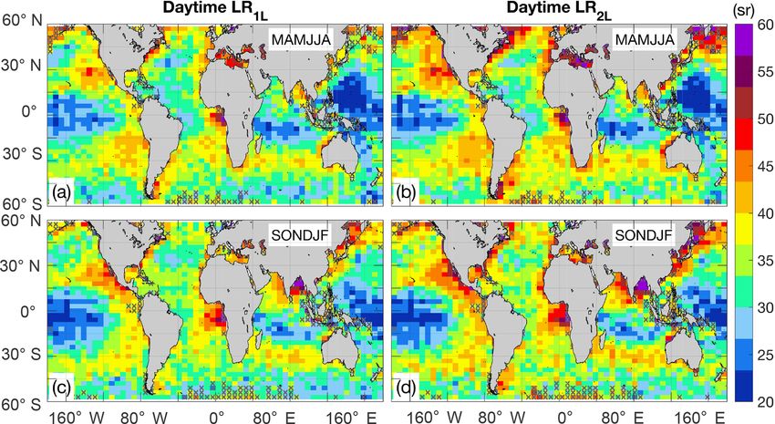
D. Painemal et al.: Aerosol extinction coefficients and lidar ratios over the ocean 2203
wavelengths. In short, SODA estimates of AOD rely on the ments, the HSRL flight paths during this campaign were
radar-to-lidar ocean surface scattering cross-calibration for spatially matched with coincident CALIPSO ground tracks
cloud-free columns (Josset et al., 2008, 2010). Consequently, (Rogers et al., 2014).
SODA can provide a cloud-free AOD without having to rely
on an accurate assignment of a particular aerosol type with
an appropriate lidar ratio. In addition, the algorithm does not 3 Derivation of aerosol extinction coefficient and lidar
depend on predetermined aerosol models with specific parti- ratio
cle size distributions and refractive indexes, unlike MODIS.
The method for deriving aerosol extinction coefficient (σa )
SODA AOD version 2, based on CALIPSO version 3 (V3),
and lidar ratio (LR) is based on Fernald (1984) applied to the
is developed at the ICARE data and services center (http:
CALIOP attenuated backscatter, and is briefly summarized in
//www.icare.univ-lille1.fr, last access: 27 December 2017)
the following. For CALIOP, the lidar equation is expressed in
in Lille (France) under the auspices of the CALIPSO mis-
terms of height z (range) as
sion and supported by the French National Centre for Space
Studies (CNES). Josset et al. (2013) estimate a systematic βatt (z) = (βm (z) + βa (z))
error in SODA AOD of 0.015 and 0.059, respectively, for
Zz
nighttime and daytime AOD. In addition, good agreement
σm z0 + σa z0 dz0 .
between SODA and MODIS has been reported in Josset et · exp −2 (1)
al. (2010, 2015), with a correlation coefficient > 0.89 and 0
a mean difference of 0.003, while Dawson et al. (2015) re- Here βatt corresponds to the CALIOP total attenuated
port a root-mean-square error of 0.03 between SODA and backscattering cross section, βm and βa denote the molec-
AERONET AOD and r = 0.59 for AERONET sites near the ular (“m”) and aerosol (“a”) backscatter coefficients, and σm
coast. Further, we also evaluate SODA AOD with HSRL data and σa are the molecular and aerosol extinction coefficients.
in Sect. 4, and compare SODA and MODIS AOD over the Since the molecular contribution can be accurately estimated
global ocean in Sect. 6. While 1064 nm SODA AOD is also using atmospheric profiles from numerical weather models,
utilized in this study, caution needs to be exercised when us- the two unknowns are βa (z) and σa (z). Equation (1) can be
ing the 1064 nm SODA data due to calibration uncertainties reduced to one unknown by relating extinction and backscat-
in CALIPSO V3 (Vaughan et al., 2010). ter coefficient via their lidar ratio, that is
2.3 HSRL σa (z)
LR(z) = . (2)
βa (z)
CALIOP retrievals are evaluated against airborne measure-
It follows that Eq. (1) can be expressed in terms of LR and
ments by the NASA Langley High Spectral Resolution Li-
βm as
dar (HSRL; Hair et al., 2008) at 532 nm. The instrument al-
lows for the independent determination of aerosol extinction βatt (Z) = (βm (z) + βa (z))
and backscatter coefficients at 532 nm (and thus lidar ratio)
Zz
using the HSRL technique (Eloranta, 2005). HSRL 532 nm
σm z0 + LR(z0 ) · βa z0 dz0 .
AOD and aerosol extinction coefficients have been regularly · exp −2 (3)
validated against other airborne instruments, with biases less 0
than 6 % and 3 %, respectively (Rogers et al., 2009), and gen-
The conventional method to solve Eq. (3) follows Fernald
erally to within 0.03 in comparison with AERONET AOD
(1984) and consists of iteratively solving for βa , assuming
(Sawamura et al., 2017). The AOD product from the HSRL
a functional form of the lidar ratio LR(z). The LR selec-
instrument makes use of the molecular channel, which is a
tion is physically constrained byR comparing the retrieved
direct observation of atmospheric attenuation between the z
aerosol optical depth (AODret = 0 σa z0 dz0 ) with SODA
aircraft and the surface when compared against the GEOS-
AOD (AODSODA ), and LR is iteratively adjusted until the
5 molecular density profile (Rogers et al., 2009). Since this
retrieved AOD matches the SODA AOD to within 0.001 or
method requires no assumptions about the lidar ratio or as-
less (i.e., when |AODret − AODSODA | ≤ 0.001). While the
sumptions that the lidar ratio is constant, it provides a useful
distribution of LR with height can be specified in different
truth measurement in the context of this study.
ways (e.g., Ansmann, 2006), here we opt for two assump-
As HSRL measurements at 1064 nm are limited to attenu-
tions, which in turn yield two independent sets of aerosol
ated backscatter, similar to CALIOP, only 532 nm HSRL re-
extinction and lidar ratio retrievals.
trievals will be utilized in this study. The data used in this
study were acquired 11–27 August 2010 while the HSRL 1. One-layer lidar ratio (1LR). The simplest assumption
conducted a dedicated CALIPSO validation campaign over is to consider one constant lidar ratio with height. This
the Caribbean Sea (Burton et al., 2013; Rogers et al., 2014). method is expected to perform well for atmospheric pro-
As required for all HSRL–CALIPSO validation measure- files characterized by only one aerosol type.
www.atmos-meas-tech.net/12/2201/2019/ Atmos. Meas. Tech., 12, 2201–2217, 2019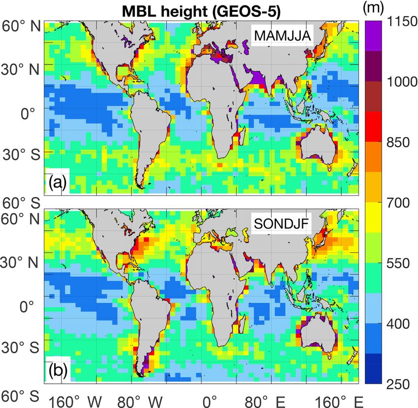
2204                                       D. Painemal et al.: Aerosol extinction coefficients and lidar ratios over the ocean

    2. Two-layer lidar ratio (2LR). We also consider an ad-
       ditional scenario, which consists of treating the atmo-
       spheric column as two layers, that is, the marine at-
       mospheric boundary layer (MBL) and a second aerosol
       layer of as-yet-undetermined composition. This method
       is intended to better capture specific events with two
       predominant aerosol types, particularly smoke over ma-
       rine aerosols and dust over marine aerosols, which are
       particularly frequent over the Atlantic Ocean. The LR
       for the MBL is assumed constant at 25 sr, as suggested
       by HSRL measurements over the ocean (Burton et al.,
       2012, 2013). This lidar ratio is slightly higher than the
       value of 23 sr assumed by Kim et al. (2018) and 18±5 sr     Figure 1. (a) Flight tracks during the 2010 field campaign (colored
                                                                   for individual flight missions). Black solid lines correspond to the
       reported by Groß et al. (2013) at Cabo Verde (14.9◦ N,
                                                                   matched CALIPSO tracks. (b) Mean HSRL lidar ratio (532 nm) as
       23.5◦ W). In contrast, 532 nm Raman lidar observations
                                                                   a function of altitude and 1 standard deviation (error bar) for all the
       at Barbados (13◦ N, 59◦ W) encompass MBL lidar ra-          flight tracks in Fig. 1a.
       tios between 21 and 35 sr, with magnitudes primarily
       controlled by free tropospheric intrusions of dust (Groß
       et al., 2015) and the environmental relative humidity
       (Haaring et al., 2017). A similar range of MBL lidar ra-    CALIOP–SODA are then spatially collocated with the air-
       tios was observed in the eastern Atlantic by Bohlmann       craft track (Fig. 1) for samples with a temporal mismatch of
       et al. (2018), with values modulated by the presence        less than 90 min (Rogers et al., 2014). Lastly, satellite and air-
       of dust–smoke aerosols. Without a priori knowledge of       borne observations are spatially averaged to a common 0.2◦
       the MBL lidar ratio, the value prescribed here (25 sr) is   resolution (in latitude). It is worth noting that although the
       within the range reported in previous studies over the      CALIOP V4 data products are reported at a uniform hor-
       ocean. σa (z) and the upper-layer LR are iteratively cal-   izontal resolution of 5 km, in reality, larger spatial averag-
       culated using the Fernald method with the constraint        ing of the lidar signal is required (20 or 80 km) for tenuous
       provided by AODSODA , and LR = 25 sr in MBL. MBL            aerosol layers to increase the aerosol layer detectability in the
       height is computed by applying the bulk Richardson          CALIPSO aerosol classification scheme. Thus, the use of a
       number method (McGraw-Spangler and Molod, 2014).            0.2◦ horizontal average for comparing airborne and satellite
                                                                   observations is adequate when considering possible spatial
The CALIOP attenuated backscatter (βatt ) at 333 m resolu-
                                                                   averaging of the CALIOP V4 retrievals. Approximately 42
tion is taken from the Level 1 CALIPSO product and av-
                                                                   and 46 0.2◦ samples were collocated with HSRL (CALIOP–
eraged to achieve a 1 km along-track resolution. Similarly,
                                                                   SODA and CALIOP, respectively).
SODA AOD retrieved at 333 m is averaged to 1 km resolu-
                                                                      The HSRL measurements during Caribbean 2010 were
tion. In addition, the feature classification mask product is
                                                                   characterized by the presence of dust, dust mixed with mar-
utilized for identifying cloudy pixels and cases with fully at-
                                                                   itime aerosols and continental pollution; the occurrence of
tenuated signal, in which CALIOP–SODA retrievals are not
                                                                   pure maritime aerosols was confined to the boundary layer
possible. The molecular components in Eq. (3) are derived
                                                                   (Burton et al., 2013). This aerosol typing is manifested in a
from the Goddard Earth Observing System Model version 5
                                                                   lidar ratio of 25 sr below 500 m and a linear increase with
(GEOS-5), with βm estimated as a function of air density, and
                                                                   height that reaches values of 40–45 sr in the free troposphere
the effect of ozone attenuation in σm is accounted for follow-
                                                                   (Fig. 1b). These measurements also provide support for the
ing Vaughan et al. (2005). Lastly, MBL height for the 2LR
                                                                   use of a lidar ratio of 25 sr in the boundary layer for the
method is also computed from GEOS-5.
                                                                   2L method. Before evaluating aerosol extinction coefficients
                                                                   and lidar ratios, we compare SODA AODs and CALIOP V4
4    CALIOP–SODA evaluation with airborne HSRL                     AODs against their HSRL counterparts (Fig. 2a). In general,
     measurements                                                  both CALIOP-based retrievals correlate well with the HSRL
                                                                   (r ≥ 0.94), with a slightly higher correlation for SODA (and
CALIOP–SODA retrievals of aerosol extinction coefficient,          absolute bias between 10 % and 17 %), with SODA underes-
lidar ratio and AOD are evaluated using eight flights dur-         timating and CALIOP V4 overestimating AOD. Linear fits
ing August 2010 over the western Atlantic, for the domain          of SODA and V4 AOD relative to HSRL (red and blue lines
bounded by 70–55◦ W and 13–35◦ N (Fig. 1a). CALIOP–                in Fig. 2a) indicate that the SODA bias is relatively con-
SODA is spatially averaged to match the nominal 5 km hor-          stant with AOD, whereas a V4 AOD overestimate tends to
izontal resolution of CALIPSO V4, and only samples with            increase with AOD especially during nighttime. Nighttime
5 km cloud-free scenes are retained. Both CALIPSO V4 and           and daytime correlations remain approximately the same for

Atmos. Meas. Tech., 12, 2201–2217, 2019                                                www.atmos-meas-tech.net/12/2201/2019/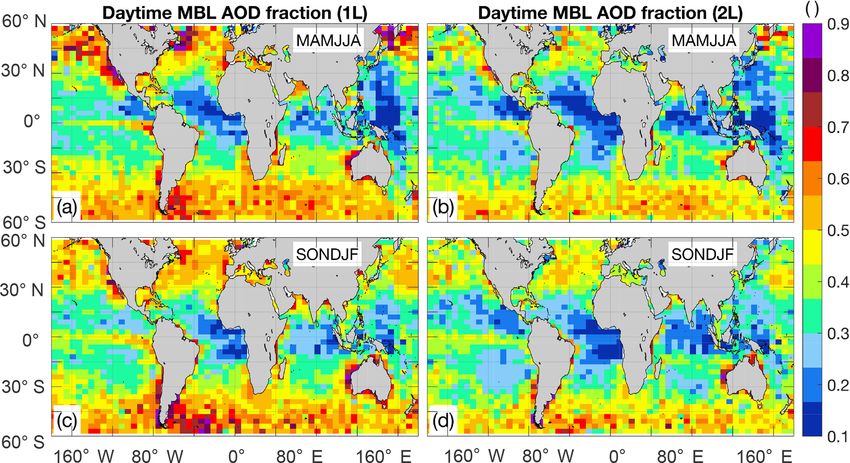
D. Painemal et al.: Aerosol extinction coefficients and lidar ratios over the ocean                                                 2205

                                                                       Table 2. As in Table 1 but for CALIOP–SODA lidar ratio.

                                                                           CALIOP–SODA           r           Mean bias            RMSE
                                                                           LR
                                                                           One layer (1L)      0.67    −2.5 sr (−8.1 %)   7.4 sr (27.1. %)
                                                                           Two layers (2L)     0.72   −4.7 sr (−17.4 %)   8.7 sr (32.0 %)

                                                                       and LRHSRL is performed by recomputing LRHSRL using the
                                                                       MBL height for z0 in Eq. (4). Since valid HSRL extinction
Figure 2. (a) Scatterplot between SODA (red) and CALIPSO V4            retrievals are only derived for heights above 270 m from the
(blue) against HSRL AOD at 532 nm. Filled and open circles in-         surface, we have assumed a constant extinction coefficient
dicate daytime and nighttime observations, respectively. Blue and      for the layer below 270 m, with values taken from the low-
red lines (and equations) are the linear fit for V4 and SODA AOD       est height with available retrievals (∼ 270 m). The compar-
(AODv4 and AODS ) relative to HSRL. (b) Comparison between
                                                                       ison depicted in Fig. 2b yields r = 0.67–0.72 between both
CALIPSO–SODA (CALS ) lidar ratio based on the one-layer (1L)
and two-layer (2L) assumptions with the HSRL column-effective
                                                                       CALIOP–SODA methods (1L and 2L) and HSRL, with a
lidar ratio from Eq. (4) (black and gray symbols, respectively). The   negative mean bias smaller than 17.4 % and RMSE of up to
gray dashed line is the one-to-one relationship.                       8.7 sr (Fig. 2b and Table 2).
                                                                          Mean vertically resolved aerosol extinction coefficients
Table 1. Linear correlation coefficient (r), mean bias and RMSE        from SODA, CALIOP V4 and HSRL are depicted in Fig. 3a
between HSRL and SODA and CALIOP standard V4 AOD. Per-                 and b for daytime and nighttime observations, respec-
centages are calculated relative to the mean HSRL AOD.                 tively. The agreement between HSRL (red) and CALIOP–
                                                                       SODA 1L and 2L (overlapped gray and black) is remark-
  CALIOP-based               r        Mean bias           RMSE         able throughout the lower troposphere, with a maximum
  AOD                                                                  overestimation of 0.027 km−1 (50 %) near 500 m. CALIOP–
                                                                       SODA 1L and 2L yield identical results, which is likely
  SODA                 0.96      −0.024 (−17 %)    0.035 (24.2 %)
                                                                       the effect of a shallow marine boundary layer (< 500 m).
  Standard V4          0.94         0.014 (10 %)   0.044 (31.2 %)
                                                                       In contrast, CALIOP V4 (blue) consistently overestimates
                                                                       the airborne measurements for heights below 1 km dur-
                                                                       ing both daytime and nighttime, with magnitudes up to
both CALIOP V4 and SODA. However, V4 linear correla-                   0.102 km−1 (100 %) relative to the HSRL during night-
tion coefficients for AOD < 0.3 are slightly lower for day-            time and 0.078 km−1 (140 %) during the day. This over-
time (r = 0.78) than nighttime (r = 0.94), whereas SODA                estimate is explained by the CALIPSO V4 constant li-
daytime–nighttime correlations for low AOD remain high                 dar ratio of 37 sr for dusty marine aerosol, which is gen-
(r ≥ 0.93). The reduced daytime correlation for CALIOP V4              erally higher than the lidar ratio retrieved by both the
is expected as the reduced signal-to-noise ratio due to the so-        HSRL and SODA for Caribbean 2010 (Fig. 2b). Inter-
lar background signal hampers the algorithm’s ability to de-           estingly, both CALIOP–SODA and CALIOP V4 correlate
tect and classify aerosols. Finally, in terms of the root-mean-        well with the HSRL, with correlations around 0.80 (Ta-
square error (RMSE), SODA RMSE (24.2 % relative to the                 ble 3). The RMSE for CALIOP V4 is also higher than
mean) is smaller than that for CALIOP V4 (31.2 %, Table 1).            that for CALIOP–SODA, especially below 1 km, with max-
   The evaluation of CALIOP–SODA lidar ratio and aerosol               ima around 0.12 km−1 (155 %) and 0.06 km−1 (83 %) for
extinction coefficient is summarized in the following. For             CALIOP V4 and CALIOP–SODA, respectively (Fig. 3c).
LR, we use the column-effective lidar ratio (Ansmann,                  Aerosol extinction coefficient statistics for the atmospheric
2006), calculated as                                                   column below 3.0 km (Table 2) corroborate the overall
             z1
             P                                                         smaller bias and RMSE of CALIOP–SODA relative to V4.
                    σa (z)
             z=z0
LRHSRL =      z1             ,                                  (4)
              P
                    βa (z)                                             5     Global analysis
            z=z0
                                                                       5.1     Preliminary comparison between CALIOP–SODA,
with z1 denoting the highest altitude with σa HSRL re-                         MODIS and CALIOP-V4 AOD
trievals (∼ 6.5 km). For evaluating CALIOP–SODA 1L LR,
LRHSRL in Eq. (4) is estimated using the last range bin above          A total of 5 months of collocated SODA, CALIOP V4 Level
the ocean surface (37.8 m) as the lower bound, z0 . In ad-             2 and Aqua MODIS data during June–October 2010 were
dition, the comparison between CALIPSO–SODA 2L LR                      compared over nonpolar oceanic regions with the goal of

www.atmos-meas-tech.net/12/2201/2019/                                                        Atmos. Meas. Tech., 12, 2201–2217, 2019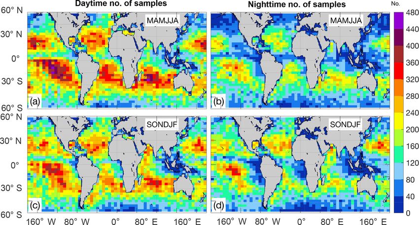
2206 D. Painemal et al.: Aerosol extinction coefficients and lidar ratios over the ocean
Figure 3. Mean aerosol extinction coefficient profile from the HSRL (red), CALIPSO–SODA 1L (black), 2L (gray) and the CALIPSO
standard V4 product (blue) during (a) daytime and (b) nighttime. (c) Total mean bias of CALIPSO-based extinction relative to the HSRL:
CALIPSO–SODA 1L (black) and 2L (gray); CALIPSO V4 (blue). Error bars in Fig. 3a and b denote 1 standard deviation, and RMSE is
shown in Fig. 3c.
Table 3. As in Table 1 but for V4 and SODA aerosol extinction coefficient in the lower troposphere (below 3.0 km).
CALIOP-based extinction r Mean bias RMSE
CALIOP V4 0.82 0.013 km−1 (33.0 %) 0.043 km−1 (106.0 %)
SODA one layer (1L) 0.78 −0.0037 km−1 (−9.2 %) 0.028 km−1 (72.6 %)
SODA two layers (2L) 0.79 −0.0029 km−1 (−7.0 %) 0.028 km−1 (73.8 %)
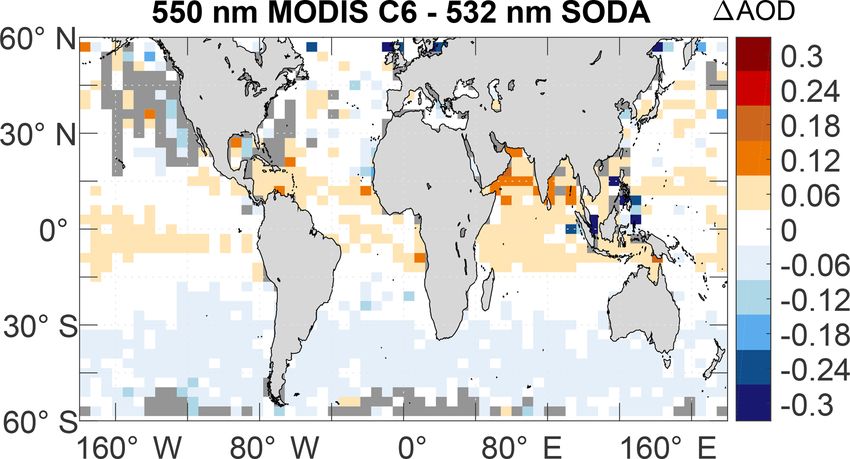
identifying the main differences in aerosol extinction coef- To verify that SODA–CALIPSO V4 differences are
ficient profiles. These months were selected because of the mainly attributed to CALIPSO V4 biases, we perform an
high global climatological AOD observed over the ocean additional comparison using Aqua MODIS Level 2 550 nm
by CALIOP (e.g., Yu et al., 2010). We first averaged 1 km AOD (MYD04_3K product), taken from the latest Collec-
CALIOP–SODA to the V4 Level 2 nominal resolution (5 km) tion 6.1 (Levy et al., 2013) for the June to October pe-
and only samples with 5 km cloud-free scenes are utilized. riod of 2010. Cloud-free 3 km MODIS AOD pixels are col-
This is intended to minimize the potential effect of overcast located with the CALIPSO track and averaged to approx-
scenes in the retrievals and aerosol swelling near the cloud imately 25 km (along track) to match the averaged 25 km
edges (Várnai and Marshak, 2011). Then, CALIOP–SODA SODA retrievals. Next, MODIS–SODA mean differences are
and CALIOP V4 data were further reduced by averaging the averaged every 6◦ × 3◦ grid, and depicted in Fig. 5. The
retrievals to a common 25 km resolution. Cloud cover was MODIS–SODA differences in Fig. 5 are typically within the
derived from the 333 m Vertical Feature Mask and deter- ±0.06 range. Although 1AOD reaches up to 0.12 over the
mined as the ratio between profiles with at least one cloudy Indian Ocean, these differences are smaller than those be-
feature in the atmospheric column to the total. To circumvent tween CALIPSO V4 and SODA (Fig. 4a). Overall, MODIS
CALIOP’s narrow field of view, we calculated the statistics further corroborates that CALIPSO V4 AOD is biased low
in 6◦ × 3◦ (longitude × latitude) grids. over regions dominated by smoke and biased high for regions
We first focus on the AOD difference (1AOD) between with dust. We note that the plausible oceanic CALIOP V4
CALIOP V4 and SODA at 532 and 1064 nm, for day and bias dependence on aerosol types suggested in our study
nighttime (Fig. 4). Daytime 532 nm 1AOD maps reveal might not be applicable over land, where AOD for dust is
higher V4 AOD than SODA for the northeast Atlantic (NEA) underestimated by CALIPSO (e.g., Schuster et al., 2012).
and the Indian Ocean (IO), whereas V4 AOD is smaller than We also show 1AOD for the 1064 nm channel in Fig. 4c,
SODA over the southeast Atlantic (SEA) and over vast re- d. The largest 1AOD values are mostly confined to the NEA
gions of the open ocean. These differences are similar to and IO domains, with higher values for CALIPSO V4 AOD
those observed between CALIOP V3 and MODIS (Rede- and similar 1AOD during daytime and nighttime.
mann et al., 2012). Overall, nighttime differences in 532 nm
AOD appear to diminish, especially for the SEA and the
northwest Pacific (NWP), while the positive 1AOD remains
high over the IO and NEA.
Atmos. Meas. Tech., 12, 2201–2217, 2019 www.atmos-meas-tech.net/12/2201/2019/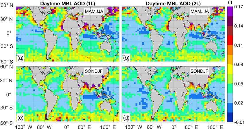
D. Painemal et al.: Aerosol extinction coefficients and lidar ratios over the ocean                                                    2207

Figure 4. Mean AOD difference between CALIOP V4 and SODA for 5 months of 2010 for daytime (a, c) and nighttime (b, d) and the
532 nm (a, b) and 1064 nm (c, d) channels. Boxes denote specific regions in which the extinction coefficient profiles are further compared in
Fig. 5: South Pacific (SP), southeast Atlantic (SEA), Indian Ocean (IO), northeast Atlantic (NEA) and northwest Pacific (NWP).

                                                                         the CALIPSO V4 overestimation during Caribbean 2010
                                                                         (Fig. 3). CALIOP–SODA and V4 profile differences are
                                                                         modest for regions with small AOD differences, such as the
                                                                         South Pacific (SP) and the northwest Pacific (NWP). An-
                                                                         other interesting aspect is the generally higher variability of
                                                                         daytime CALIPSO V4 relative to SODA, manifested in the
                                                                         high standard deviations in Fig. 6 (error bars). This indicates
                                                                         that SODA retrievals are more stable than CALIPSO V4,
                                                                         especially during the daytime, due to the AOD constraint.
                                                                         Moreover, the high solar background substantially degrades
                                                                         CALIPSO aerosol detection capabilities, affecting the re-
                                                                         trieved extinction. Lastly, CALIOP–SODA differences be-
Figure 5. Mean AOD difference between matched 550 nm MODIS
                                                                         tween 1L and 2L are small and typically confined to a layer
C6 and 532 nm SODA daytime AOD for 5 months of 2010. Oceanic
                                                                         below 700 m, where 2L tends to be smaller than 1L. This is
regions with no available MODIS samples that meet the matching
criteria are depicted in dark gray.                                      explained, as in Sect. 4, by a relatively shallow mixed-layer
                                                                         height (< 500 m), where LR = 25 sr for the 2L method.
                                                                            For completeness, in Fig. 7 we show the aerosol extinc-
                                                                         tion profiles for the 1064 nm channel. CALIOP–SODA and
5.2   CALIOP–SODA and CALIOP V4 aerosol                                  V4 profiles yield smaller differences relative to their 532 nm
      extinction profiles                                                counterpart, in agreement with 1AOD (Fig. 4).
Matched CALIOP–SODA and CALIOP V4 mean vertical                          5.3   Maps of CALIOP–SODA lidar ratio (LR) at
profiles of aerosol extinctions over the regions defined in                    532 nm
Fig. 4 (black boxes) are shown in Figs. 6 and 7, for the 532
and 1064 nm channels, respectively. The main differences, in             The number of 25 km samples utilized in the following
agreement in AOD differences in Fig. 4, are found: (a) over              SODA LR analysis is depicted in Fig. 8. The extratropical re-
the IO and NEA where CALIPSO V4 extinction profiles are                  gions yield the smallest number of samples (< 80), whereas
higher than CALIOP–SODA, and (b) over SEA, with lower                    the occurrence of clear-sky scenes is the highest over sub-
V4 extinctions than CALIOP–SODA. Even though the main                    tropical open ocean, with ∼ 400 retrievals (note that approxi-
V4–SODA differences in extinction decrease during night-                 mately at least eight 1 km samples are contained in one 25 km
time, especially over the SEA, the nighttime differences for             averaged sample with cloud fraction < 67 %). During night-
the NEA and IO remain nearly the same. Interestingly, the                time, the number substantially decreases due to the cloud di-
higher CALIOP V4 extinction for the NEA and IO resembles                 urnal cycle. Figures 9 and 10 depict global maps of 532 nm

www.atmos-meas-tech.net/12/2201/2019/                                                       Atmos. Meas. Tech., 12, 2201–2217, 2019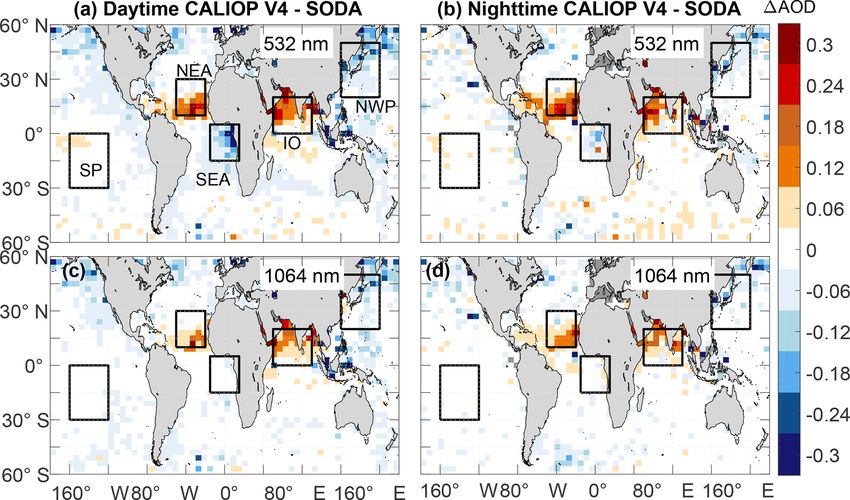
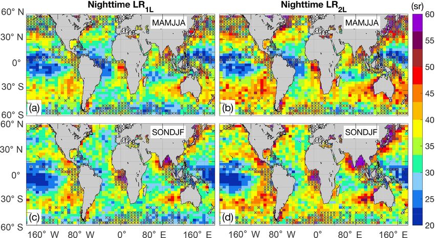
2208                                         D. Painemal et al.: Aerosol extinction coefficients and lidar ratios over the ocean

Figure 6. Mean aerosol extinction coefficient at 532 nm for the five regions defined in Fig. 4. Upper and lower panels correspond to daytime
and nighttime retrievals. CALIPSO–SODA profiles are in black (1L) and blue (2L), and CALIPSO V4 is in red.

Figure 7. As in Fig. 6 but for the 1064 nm channel.

LR derived from the 1L (LR1L ) and 2L (LR2L ) assumptions,              coast. The lowest values are observed over the western and
temporally averaged from March to August (MAMJJA, bo-                   central equatorial Pacific, with ratios less than 30 sr, which
real spring–summer) and September to February (SONDJF,                  are typical of clean maritime environments (e.g., Burton et
boreal autumn–winter) of 2010 from the 25 km averaged re-               al., 2013). Semiannual transitions are primarily found near
trievals with cloud fraction less than 67 %. Daytime 532 nm             the continents, namely, the southeast Atlantic, Mediterranean
LR exhibits a clear spatial pattern with high values (> 45 sr)          Sea, Indian Ocean and off the coast of eastern Asia. Night-
in coastal regions, especially off the southwestern African             time LRs (Fig. 10) are similar to their daytime counterparts,

Atmos. Meas. Tech., 12, 2201–2217, 2019                                                     www.atmos-meas-tech.net/12/2201/2019/
D. Painemal et al.: Aerosol extinction coefficients and lidar ratios over the ocean                                           2209

Figure 8. Number of 25 km CALIOP–SODA samples contained in each semiannual average: (a) daytime MAMJJA, (b) nighttime MAMJJA,
(c) daytime SONDJF and (d) nighttime SONDJF.

Figure 9. Semiannual daytime 532 nm lidar ratios. (a) LR1L for spring–summer, (b) LR2L for spring–summer, (c) LR1L for autumn–winter
and (d) LR2L for autumn–winter. Gray crosses indicate regions where less than 15 % of the maximum observable number of samples
contribute to the average.

but with slightly higher values and a rather heterogeneous          derives. Overall, LR1L and LR2L differences are relatively
pattern, attributed to the reduced cloud-free sampling at night     small (∼ 5 sr), which, as we will show in the next section, is
due to the increased cloud cover, especially over subtropical       associated with the shallow MBL height estimated from the
regions and the Southern Ocean (Fig. 8b and d), where strat-        bulk Richardson number method and therefore a relatively
iform and shallow cumulus clouds are abundant.                      small fraction of aerosol that is controlled by the assumed
   Comparing the two-layer assumptions, LR2L (Fig. 9b and           marine lidar ratio in the 2L method.
d) is higher than LR1L , especially for lidar ratios > 40 sr.
This result is expected, as the prescribed MBL lidar ratio of       5.4   Fractional CALIOP–SODA AOD at 532 nm in the
25 sr for 2L tends to be lower than the lidar ratio for any               marine boundary layer
aerosol type that would be found above the marine bound-
ary layer and therefore lower than the column average or
                                                                    CALIOP–SODA aerosol extinctions are further utilized for
column-effective lidar ratio. Therefore, to match the SODA
                                                                    quantifying AOD in the boundary layer. We first show in
AOD, the lidar ratio above the MBL in the 2L case must
                                                                    Fig. 11 the 2010 semiannual total SODA AOD for daytime
be larger than the column-effective value that the 1L case
                                                                    (Fig. 11a, c) and nighttime (Fig. 11b, d) CALIPSO over-

www.atmos-meas-tech.net/12/2201/2019/                                                 Atmos. Meas. Tech., 12, 2201–2217, 2019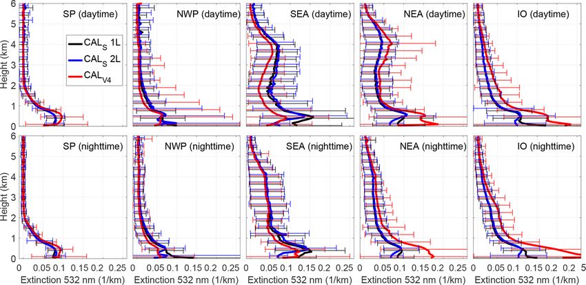
2210                                         D. Painemal et al.: Aerosol extinction coefficients and lidar ratios over the ocean

Figure 10. As in Fig. 9 but for nighttime.

passes. Consistent with several studies (e.g., Kittaka et al.,       mulus clouds. Thus, the MBL used here is expected to pri-
2011; Redemann et al., 2012), high AOD primarily occurs              marily represent the mixed-layer height (von Engeln and
over the eastern Atlantic, in connection with biomass burn-          Teixeira, 2013).
ing and dust emissions from southern and equatorial Africa.             The fraction of MBL AOD relative to the total is depicted
A second region of interest encompasses most of the Asian            in Fig. 14. The extratropical bands show the highest fraction
coastal region, where a combination of pollution and dust            of MBL AOD, accounting for up to 0.73 (73 %) of the total
gives rise to high AOD (Itahashi et al., 2010).                      AOD. Low fractions are found in the subtropics and trop-
   Before presenting MBL AOD, we show the MBL height                 ics, with the lowest AOD fraction over the eastern Atlantic
maps (Fig. 12), with typical heights below 800 m, and lit-           and the west-central Pacific. Interestingly, vast areas over the
toral maxima up to 1150 m in northern Africa and Eurasia.            ocean feature AOD fractions of less than 40 %, suggesting a
Next, we compute MBL AOD by numerically integrating                  significant contribution of free tropospheric aerosols to the
CALIOP–SODA aerosol extinction coefficient from the sur-             total AOD. These results are qualitatively consistent with
face to the MBL height. MBL AOD in Fig. 13 shows a dis-              the results of Bourgeois et al. (2018) using CALIPSO ver-
similar pattern relative to its total AOD counterpart (Fig. 11),     sion 4.1.
manifested in a less dominant role of the southeast Atlantic.
In addition, coastal Africa, Eurasia and North America ex-
hibit peaks in MBL AOD (> 0.12) during boreal spring–                6   Discussion
summer. A second region with high AOD encompasses the
extratropical oceans poleward of 45◦ S–N, with a particu-            One of the few global satellite-based estimates of lidar ratio
larly consistent zonal band with high AOD in the Southern            is reported in Bréon (2013), who estimated LR utilizing the
Ocean. As expected, 2L MBL AOD is lower than 1L due                  retrieved scattering phase function at a 180◦ angle derived
to the 2L assumption of a lidar ratio equal to 25 sr in the          from the Polarization and Directionality of the Earth’s Re-
MBL. Except for the subtropical ocean, which features shal-          flectances (POLDER) satellite instrument and a prescribed
low MBL and low MBL AOD, a spatial modulation of the                 aerosol model. POLDER LR and CALIOP–SODA (Figs. 9–
marine boundary layer in the MBL AOD is unclear. It is im-           10) yield high LR over the coasts of eastern Africa and
portant to mention that estimates of the AOD apportioned             Eurasia and a notable increase in LR over the Indian Ocean
in the boundary layer will depend on the MBL dataset uti-            in boreal autumn–winter. In addition, both POLDER and
lized in the calculations. An alternative MBL height estima-         CALIOP–SODA produce LR < 30 sr over the open ocean.
tion derived from CALIOP attenuated backscatter (McGrath-            Conversely, LRs from POLDER tend to be slightly higher,
Spangler and Denning, 2013) yields similar if not higher val-        with a typical range between 30 and 70 sr. Bréon (2013) also
ues than our GEOS-based MBL. However, MBL estimates                  indicates that because POLDER retrievals rely on scattered
based on thermodynamical vertical profiles (temperature, rel-        photon measurements, LR might be biased low in regions
ative humidity) from meteorological analyses produce signif-         dominated by absorbing aerosol, such as the southeast At-
icantly higher MBL (von Engeln and Teixeira, 2013), closely          lantic. A somewhat different method of retrieving LR from
matching the cloud-top height of stratiform and shallow cu-          SODA AOD, documented in Josset et al. (2011), consists
                                                                     of analytically solving the lidar equation. The only avail-

Atmos. Meas. Tech., 12, 2201–2217, 2019                                                www.atmos-meas-tech.net/12/2201/2019/
D. Painemal et al.: Aerosol extinction coefficients and lidar ratios over the ocean 2211
Figure 11. SODA AOD for daytime (a, c) and nighttime (b, d) spring–summer (MAMJJA) and autumn–winter (SONDJF). Gray crosses are
described in Fig. 9.
lowing lidar ratios for a number of aerosol types: the highest
LRs (45–80 sr) are typically attributed to smoke and urban
aerosols, LRs of 25–50 and 40 sr are associated with dust
and polluted maritime aerosols (respectively), and maritime
aerosols are characterized by lidar ratios of less than 30 sr.
For simplicity, we will primarily interpret daytime LR1L in
Fig. 9a and c for the following regions of interest.
6.1 Southeast Atlantic
The SODA LR peak in the southeast Atlantic is explained
by the well-documented biomass burning season over south-
ern Africa, with massive fire events from May to September
during the dry season (Roberts et al., 2009) and smoke be-
ing transported offshore by the prevailing winds from July
to October (Adebiyi et al., 2015). HSRL airborne measure-
ments collected in September 2016 (Burton et al., 2018)
show 532 nm LRs in the range 58–76 sr in the free tropo-
sphere, with CALIOP–SODA yielding values in the lower
bound of the HSRL measurements (55–60 sr). In addition,
shipborne Raman lidar observations south of the region dom-
Figure 12. Daytime marine boundary layer height for (a) spring–
inated by biomass burning aerosols (30◦ S, near the South
summer and (b) autumn–winter.
African coast) reveal a transition from a lower troposphere
dominated by smoke to one mainly composed of maritime
aerosols (lidar ratios less than 25 sr; Bohlmann et al., 2018).
able global analysis of LR using the technique in Josset et This southward reduction in LR is reproduced by CALIOP–
al. (2011) is documented in Dawson et al. (2015) for mar- SODA.
itime aerosols only, reporting values between 20 and 40 sr.
As different aerosol types can be, to some extent, charac- 6.2 Mediterranean Sea
terized by their lidar ratio, the reliability of CALIOP–SODA
LR retrievals is qualitatively assessed by analyzing the con- The high spring–summer SODA LR over the Mediterranean
sistency between the CALIOP–SODA LR spatial pattern and Sea (∼ 50 sr) is also expected given the southward pollu-
the regional occurrence of aerosol types as well as lidar mea- tion transport from Europe, which is maximized in sum-
surements from several field campaigns over the ocean. Bur- mer in the boundary layer (Duncan and Bey, 2004). More-
ton et al. (2012), using HSRL measurements over North over, lidar observations show a maximum dust AOD over
America and the adjacent Atlantic Ocean, provide the fol- the Mediterranean Sea (southern Italy) in summer (Mona
www.atmos-meas-tech.net/12/2201/2019/ Atmos. Meas. Tech., 12, 2201–2217, 20192212 D. Painemal et al.: Aerosol extinction coefficients and lidar ratios over the ocean
Figure 13. Daytime MBL 532 nm AOD based on 1L (a, c) and 2L (b, d).
Figure 14. Fraction of daytime AOD contributed by the marine boundary layer.
et al., 2006), in connection with a Saharan dust layer in Korea, a semiannual contrast is retrieved by SODA, with
the free troposphere. The higher presence of pollution and maximum LR > 55 sr for SONDJF. Changes between au-
dust in spring would explain the high CALIOP–SODA LR tumn and spring were also observed over the Korean penin-
in spring–summer (MAMJJA). sula in the lidar ratios retrieved with a Raman lidar (Noh et
al., 2008), with layer mean of 56 and 63 sr for spring and
6.3 Bay of Bengal and western Pacific Ocean autumn, respectively, and larger differences in the free tropo-
sphere. These changes are thought to be primarily explained
by seasonal changes in the composition of dust and smoke.
A major LR maximum in autumn–winter (SONDJF) is ob-
served south of India, over the Bay of Bengal and part of
the Arabian Sea. This pattern is concomitant with the perva- 6.4 Eastern Pacific and Southern Ocean
sive presence of pollution and biomass burning during the
winter and pre-monsoon season (October to April; Krish- Regions with intermediate CALIOP–SODA LR (35 sr <
namurti et al., 2009). In contrast, during the monsoon sea- LR < 50 sr) are located over broad regions of the eastern Pa-
son (June–September), dust aerosols become the dominant cific and the east coast of North America. These regions are
species over the Bay of Bengal (Das et al., 2013), which is likely influenced by a combination of maritime aerosols and
manifested in the reduction in SODA LR in spring–summer pollution from the continents. It is nevertheless surprising
(MAMJJA). Further east, off the coast of eastern China and that high SODA lidar ratios are retrieved over rather pristine
Atmos. Meas. Tech., 12, 2201–2217, 2019 www.atmos-meas-tech.net/12/2201/2019/D. Painemal et al.: Aerosol extinction coefficients and lidar ratios over the ocean 2213
regions, especially over the Southern Ocean, where maritime pecially when considering the sometimes large differences
aerosols are expected to be the dominant aerosol type. A between SODA and MODIS AOD (> 0.06, Fig. 5). To as-
plausible factor that may help reconcile high LR for maritime sess the uncertainty in the retrieved CALIOP–SODA LR at-
aerosols is a lidar ratio increase with relative humidity (Ack- tributed to errors in SODA AOD, we assume a ±20 % pertur-
erman, 1998). Relative humidity could also explain the pres- bation in SODA AOD and estimated LR. A 20 % AOD error
ence of LR > 30 sr over stratocumulus cloud regimes, where is similar to the 24 % RMSE between SODA and the airborne
high relative humidity is confined in the boundary layer. HSRL AOD (Sect. 4). For one CALIPSO overpass we found
that a 20 % higher SODA AOD gives rise to a 5.4 sr increase
6.5 Central Pacific and northern Atlantic in lidar ratio, or equivalent to a 14.4 % lidar ratio change rela-
tive to the LR constrained with unperturbed AOD. Similarly,
The regions with the lowest LR are located over the tropi- a 20 % lower SODA AOD yields a 6.0 sr decrease in lidar
cal Pacific Ocean, where AOD is the lowest (Fig. 11). An ratio (−16.0 %). These results are analogous to the 1AOD
unanticipated result is the absence of a zonal band across the uncertainty of 18 % (for AOD = 0.15) attributed to a 15 %
Atlantic that could be attributed to the westward transport of error in the lidar ratio prescribed by the CALIPSO algorithm,
Saharan dust across the Atlantic Ocean. Unfortunately, due to derived using the AOD error equation in Winker et al. (2009).
the lack of in situ observations along the Saharan dust path-
ways, the assessment of SODA LR over this region is chal-
lenging. Raman lidar data over the eastern Atlantic (Cape 7 Concluding remarks
Verde), off the coast of western Africa, in spring show dust
A total of 1 year of a new CALIOP-based aerosol extinc-
and smoke in the free troposphere and boundary layer with a
tion coefficient and lidar ratio dataset has been presented,
mean LR of 54 sr (Tesche et al., 2011) and a dust layer thick-
with the goal of providing a flexible dataset for climate re-
ness of about 4 km. Over the same region, SODA LR is 40 sr,
search as well as independent retrievals that can be helpful
which increases up to 45–50 sr when LR is estimated using
for refining CALIPSO Science Team algorithms. The new re-
the 2L assumption. Ground-based lidar observations over the
trievals build on the CALIPSO V4 total attenuated backscat-
western Atlantic (Barbados, 13.14◦ N, 59.62◦ W) in summer
ter and cloud mask data products. However, the method that
reveal the presence of maritime aerosols and dust, with lidar
we used to invert the lidar equation differs fundamentally
ratios of less than 40 sr in the boundary layer, and pure dust
from the CALIOP standard aerosol product, as it does not
aerosols generally confined to the free troposphere (Groß et
rely upon an aerosol classification module to prescribe the
al., 2015). This suggests that the relatively low CALIOP–
lidar ratio. We evaluated CALIOP–SODA AOD, LR and
SODA LR over the Atlantic basin may be explained by the
extinction using airborne HSRL retrievals over the western
contribution of maritime aerosols in the boundary layer. A
Atlantic, and found excellent agreement, with statistically
more quantitative assessment, which includes the analysis of
significant correlations (r ≥ 0.67) and biases around 27 %–
specific dust events, is left for future work. Lastly, interpre-
32 %. Given these encouraging results, we envision potential
tation of the 1064 nm CALIOP–SODA is not attempted here
uses of CALIOP–SODA lidar ratios for evaluating CALIOP
due to the lack of independent measurements and calibra-
V4 aerosol properties. This can be carried out similar to Daw-
tion uncertainties associated with the use of CALIPSO V3
son et al. (2015), by stratifying CALIOP–SODA LR as a
for deriving SODA AOD. A future release of SODA based
function of CALIOP V4 aerosol types and their assigned li-
on CALIPSO V4 will benefit from the improved calibration
dar ratio.
of V4, which is estimated to be within 3 % (Vaughan et al.,
Although the retrievals presented here are limited to cloud-
2019).
free atmospheric columns due to the constraint imposed by
An aspect that deserves further discussion is the reliability
SODA AOD, it is possible to adapt the algorithm to make
of SODA AOD, as it is essential for constraining the lidar
use of above-cloud satellite AOD retrievals (e.g., Jethva et
equation in our study. We find a high linear correlation be-
al., 2014; Liu et al., 2015). In this regard, above-cloud AOD
tween SODA and HSRL AOD (r = 0.96), with no clear rela-
using CALIOP can be derived by combining the integrated
tionship between SODA biases and AOD magnitudes, and a
attenuated backscatter and depolarization ratio (Hu et al.,
SODA-to-HSRL RMSE comparable to the one estimated be-
2007; Liu et al., 2015) with corrections for the multiple-
tween SODA and AERONET in Dawson et al. (2015). The
scattering depolarization relationship implemented by SODA
differences between SODA, CALIPSO V4 and MODIS AOD
(Deaconu et al., 2017). Efforts to retrieve above-cloud lidar
(Figs. 4 and 5) also support inferences based on compar-
ratio and extinction profiles over the southeast Atlantic using
isons between MODIS and CALIPSO Science Team AOD
the above-cloud AOD are currently underway (Ferrare et al.,
over the ocean (Redemann et al., 2012; Kim et al., 2013).
2018).
Redemann et al. (2012) and our results both point to an over-
estimation of CALIPSO V4 AOD over oceanic regions dom-
inated by dust and an underestimation in regions dominated
by smoke. However, errors in SODA AOD are plausible, es-
www.atmos-meas-tech.net/12/2201/2019/ Atmos. Meas. Tech., 12, 2201–2217, 20192214 D. Painemal et al.: Aerosol extinction coefficients and lidar ratios over the ocean
CALIOP–SODA 1L retrievals are expected to perform References
better for relatively homogeneous atmospheric profiles char-
acterized by a single aerosol type. Alternatively, SODA 2L Ackermann, J.: The Extinction-to-Backscatter Ratio of Tro-
retrievals are likely to be advantageous for specific regions pospheric Aerosol: A Numerical Study, J. Atmos. Ocean.
Tech., 15, 1043–1050, https://doi.org/10.1175/1520-
where massive aerosol plumes from the continent are trans-
0426(1998)0152.0.CO;2, 1998.
ported offshore at high altitudes through convective pro- Adebiyi, A. A., Zuidema, P., and Abel, S. J.: The Convolution of
cesses, in such a way that MBL aerosols are detached from Dynamics and Moisture with the Presence of Shortwave Absorb-
the layer above and the assumption MBL LR = 25 sr (mar- ing Aerosols over the Southeast Atlantic, J. Climate, 28, 1997–
itime) is a good approximation. This is probably the case over 2024, https://doi.org/10.1175/JCLI-D-14-00352.1, 2015.
the southeast Atlantic during the biomass burning season or Ansmann, A.: Ground-truth aerosol lidar observations: can the Klett
for episodic dust transport over the tropical Atlantic. How- solutions obtained from ground and space be equal for the same
ever, the CALIPSO Science Team product will continue pro- aerosol case?, Appl. Optics, 45, 3367–3371, 2006.
viding the best available global dataset for monitoring com- Bohlmann, S., Baars, H., Radenz, M., Engelmann, R., and
plex aerosol profiles, continental processes and aerosols in Macke, A.: Ship-borne aerosol profiling with lidar over the
the upper troposphere. Atlantic Ocean: from pure marine conditions to complex
dust–smoke mixtures, Atmos. Chem. Phys., 18, 9661–9679,
https://doi.org/10.5194/acp-18-9661-2018, 2018.
Bourgeois, Q., Ekman, A. M. L., Renard, J.-B., Krejci, R., Dev-
Data availability. CALIPSO version 4.1 is available at
asthale, A., Bender, F. A.-M., Riipinen, I., Berthet, G., and
https://eosweb.larc.nasa.gov (last access: 17 January 2019) –
Tackett, J. L.: How much of the global aerosol optical depth
https://doi.org/10.5067/CALIOP/CALIPSO/LID_L2_05kmAPro-
is found in the boundary layer and free troposphere?, Atmos.
Standard-V4-10 (Vaughan et al., 2019b), and SODA aerosol optical
Chem. Phys., 18, 7709–7720, https://doi.org/10.5194/acp-18-
depth is available at http://www.icare.univ-lille1.fr/projects/soda
7709-2018, 2018.
(last access: 27 December 2017; Josset et al., 2015).
Bréon, F.-M.: Aerosol extinction-to-backscatter ratio derived from
passive satellite measurements, Atmos. Chem. Phys., 13, 8947–
8954, https://doi.org/10.5194/acp-13-8947-2013, 2013.
Author contributions. MC, RF, DJ and SB developed the algo- Burton, S. P., Ferrare, R. A., Hostetler, C. A., Hair, J. W., Kittaka,
rithms for retrieving aerosol extinction coefficient and lidar ratio, C., Vaughan, M. A., Obland, M. D., Rogers, R. R., Cook, A. L.,
with inputs from DP. DP conducted the analysis and wrote the pa- Harper, D. B., and Remer, L. A.: Using airborne high spectral
per with contributions from all the co-authors. resolution lidar data to evaluate combined active plus passive re-
trievals of aerosol extinction profiles, J. Geophys. Res.-Atmos.,
115, D00H15, https://doi.org/10.1029/2009jd012130, 2010.
Competing interests. The authors declare that they have no conflict Burton, S. P., Ferrare, R. A., Hostetler, C. A., Hair, J. W., Rogers, R.
of interest. R., Obland, M. D., Butler, C. F., Cook, A. L., Harper, D. B., and
Froyd, K. D.: Aerosol classification using airborne High Spectral
Resolution Lidar measurements – methodology and examples,
Acknowledgements. This work was funded by the Cloud- Atmos. Meas. Tech., 5, 73–98, https://doi.org/10.5194/amt-5-73-
Sat and CALIPSO Science Recompete Program NASA 2012, 2012.
award no. NNH16CY04C. The SODA product is de- Burton, S. P., Ferrare, R. A., Vaughan, M. A., Omar, A. H.,
veloped at the AERIS/ICARE data and services cen- Rogers, R. R., Hostetler, C. A., and Hair, J. W.: Aerosol
ter (http://www.icare.univ-lille1.fr/projects/soda, last access: classification from airborne HSRL and comparisons with the
27 December 2017) in Lille (France) in the frame of the CALIPSO CALIPSO vertical feature mask, Atmos. Meas. Tech., 6, 1397–
mission and supported by CNES. The AERIS data infrastructure 1412, https://doi.org/10.5194/amt-6-1397-2013, 2013.
is greatly acknowledged for data, processing and development Burton, S. P., Hostetler, C. A., Cook, A. L., Hair, J. W., Seaman, S.
supports of the SODA product. T., Scola, S., Harper, D. B., Smith, J. A., Fenn, M. A., Ferrare, R.
We thank Gregory Schuster for his insightful comments and sug- A., Saide, P. E., Chemyakin, E. V., and Müller, D.: Calibration of
gestions and Jacques Pelon for fruitful discussions related to the a high spectral resolution lidar using a Michelson interferometer,
SODA product and algorithms. with data examples from ORACLES, Appl. Optics, 57, 6061–
6075, 2018.
Das, S., Dey, S., Dash, S. K., and Basil, G.: Examining mineral dust
Financial support. This research has been supported by the NASA transport over the Indian subcontinent using the regional climate
(grant no. NNH16CY04C). model, RegCM4.1, Atmos. Res., 134, 64–76, 2013.
Das, S., Harshvardhan, H., Bian, H., Chin, M., Curci, G., Protono-
tariou, A. P., Mielonen, T., Zhang, K., Wang, H., and Liu, X.:
Biomass burning aerosol transport and vertical distribution over
Review statement. This paper was edited by Ulla Wandinger and
the South African-Atlantic region, J. Geophys. Res.-Atmos., 122,
reviewed by two anonymous referees.
6391–6415, https://doi.org/10.1002/2016JD026421, 2017.
Dawson, K. W., Meskhidze, N., Josset, D., and Gassó, S.: Space-
borne observations of the lidar ratio of marine aerosols, At-
Atmos. Meas. Tech., 12, 2201–2217, 2019 www.atmos-meas-tech.net/12/2201/2019/D. Painemal et al.: Aerosol extinction coefficients and lidar ratios over the ocean 2215
mos. Chem. Phys., 15, 3241–3255, https://doi.org/10.5194/acp- Itahashi, S., Yumimoto, K., Uno, I., Eguchi, K., Take-
15-3241-2015, 2015. mura, T., Hara, Y., Shimizu, A., Sugimoto, N., and Liu,
Deaconu, L. T., Waquet, F., Josset, D., Ferlay, N., Peers, F., Z.: Structure of dust and air pollutant outflow over East
Thieuleux, F., Ducos, F., Pascal, N., Tanré, D., Pelon, J., and Asia in the spring, Geophys. Res. Lett., 37, L20806,
Goloub, P.: Consistency of aerosols above clouds character- https://doi.org/10.1029/2010GL044776, 2010.
ization from A-Train active and passive measurements, At- Jethva, H., Torres, O., Waquet, F., Chand, D., and Hu, Y.: How
mos. Meas. Tech., 10, 3499–3523, https://doi.org/10.5194/amt- do A-train sensors intercompare in the retrieval of above-cloud
10-3499-2017, 2017. aerosol optical depth? A case study-based assessment, Geophys.
de Laat, A. T. J., Stein Zweers, D. C. , Boers, R., and Tuinder, O. N. Res. Lett., 41, 186–192, https://doi.org/10.1002/2013GL058405,
E.: A solar escalator: Observational evidence of the self-lifting of 2014.
smoke and aerosols by absorption of solar radiation in the Febru- Josset, D., Pelon, J., Protat, A., and Flamant, C.: New approach to
ary 2009 Australian Black Saturday plume, J. Geophys. Res., determine aerosol optical depth from combined CALIPSO and
117, D04204, https://doi.org/10.1029/2011JD017016, 2012. CloudSat ocean surface echoes, Geophys. Res. Lett., 35, L10805,
Duncan, B. N. and Bey, I.: A modeling study of the export https://doi.org/10.1029/2008GL033442, 2008.
pathways of pollution from Europe: Seasonal and interan- Josset, D., Pelon, J., and Hu, Y.: Multi-instrument cali-
nual variations (1987–1997), J. Geophys. Res., 109, D08301, bration method based on a multiwavelength ocean sur-
https://doi.org/10.1029/2003JD004079, 2004. face model, IEEE Geosci. Remote S., 7, 195–199,
Eloranta, E. W.: High spectral resolution lidar, in: Lidar. Range- https://doi.org/10.1109/LGRS.2009.2030906, 2010.
Resolved Optical Remote Sensing of the Atmosphere, edited by: Josset, D., Rogers, R., Pelon, J., Hu, Y., Liu, Z., Omar, A., and Zhai,
Weitkamp, C., 143–163, Springer, New York, 2005. P.: CALIPSO lidar ratio retrieval over the ocean, Opt. Express,
Fernald, F. G.: Analysis of atmospheric lidar observa- 19, 18696–18706, 2011.
tions: Some comments, Appl. Optics, 23, 652–653, Josset, D., Tanelli, S., Hu, Y., Pelon, J., and Zhai, P.: Analysis of wa-
https://doi.org/10.1364/AO.23.000652, 1984. ter vapor correction for CloudSat W-band radar, IEEE T. Geosci.
Ferrare, R., Burton, S., Cook, A. L., Harper, D. B., Hostetler, C., Remote, 51, 3812–3825, 2013.
Hair, J., Clayton, M., Vaughan, M., Hu, Y., Fenn, M., Josset, D., Josset, D., Hou, W., Pelon, J., Hu, Y., Tanelli, S., Ferrare, R., Burton,
Redemann, J., and da Silva, A.: CALIOP and Airborne HSRL-2 S., and Pascal, N.: Ocean and polarization observations from ac-
Measurements of Smoke above low clouds during ORACLES, tive remote sensing: atmospheric and ocean science applications,
CloudSat/CALIPSO Annual Science Review, 23–25 April 2018, Proc. SPIE 9459, Ocean Sensing and Monitoring VII, 94590N,
Boulder, Colorado, USA, 2018. https://doi.org/10.1117/12.2181544, 2015.
Gravseth, I. J. and Piepe, B.: CloudSat’s return to the A-Train, Inter- Khaykin, S. M., Godin-Beekmann, S., Hauchecorne, A., Pelon,
national Journal of Space Science and Engineering, 1, 410–431, J., Ravetta, F., and Keckhut, P.: Stratospheric smoke with
https://doi.org/10.1504/IJSPACESE.2013.059269, 2013. unprecedentedly high backscatter observed by lidars above
Groß, S., Esselborn, M., Weinzierl, B., Wirth, M., Fix, A., and Pet- southern France, Geophys. Res. Lett., 45, 1639–1646,
zold, A.: Aerosol classification by airborne high spectral reso- https://doi.org/10.1002/2017GL076763, 2018.
lution lidar observations, Atmos. Chem. Phys., 13, 2487–2505, Kim, M.-H., Kim, S.-W., Yoon, S.-C., and Omar, A. H.: Com-
https://doi.org/10.5194/acp-13-2487-2013, 2013. parison of aerosol optical depth between CALIOP and
Groß, S., Freudenthaler, V., Schepanski, K., Toledano, C., MODIS-Aqua for CALIOP aerosol subtypes over the
Schäfler, A., Ansmann, A., and Weinzierl, B.: Optical prop- ocean, J. Geophys. Res.-Atmos., 118, 13241–13252,
erties of long-range transported Saharan dust over Barba- https://doi.org/10.1002/2013JD019527, 2013.
dos as measured by dual-wavelength depolarization Raman li- Kim, M.-H., Omar, A. H., Vaughan, M. A., Winker, D. M., Trepte,
dar measurements, Atmos. Chem. Phys., 15, 11067–11080, C. R., Hu, Y., Liu, Z., and Kim, S.-W.: Quantifying the low
https://doi.org/10.5194/acp-15-11067-2015, 2015. bias of CALIPSO’s column aerosol optical depth due to unde-
Haarig, M., Ansmann, A., Gasteiger, J., Kandler, K., Althausen, D., tected aerosol layers, J. Geophys. Res.-Atmos., 122, 1098–1113,
Baars, H., Radenz, M., and Farrell, D. A.: Dry versus wet marine https://doi.org/10.1002/2016JD025797, 2017.
particle optical properties: RH dependence of depolarization ra- Kim, M.-H., Omar, A. H., Tackett, J. L., Vaughan, M. A., Winker,
tio, backscatter, and extinction from multiwavelength lidar mea- D. M., Trepte, C. R., Hu, Y., Liu, Z., Poole, L. R., Pitts, M. C.,
surements during SALTRACE, Atmos. Chem. Phys., 17, 14199– Kar, J., and Magill, B. E.: The CALIPSO version 4 automated
14217, https://doi.org/10.5194/acp-17-14199-2017, 2017. aerosol classification and lidar ratio selection algorithm, At-
Hair, J. W., Hostetler, C. A., Cook, A. L., Harper, D. B., Fer- mos. Meas. Tech., 11, 6107–6135, https://doi.org/10.5194/amt-
rare, R. A., Mack, T. L., Welch, W., Izquierdo, L. R., and Ho- 11-6107-2018, 2018.
vis, F. E.: Airborne high spectral resolution lidar for pro- fil- Kittaka, C., Winker, D. M., Vaughan, M. A., Omar, A., and Remer,
ing aerosol optical properties, Appl. Optics, 47, 6734–6752, L. A.: Intercomparison of column aerosol optical depths from
https://doi.org/10.1364/AO.47.006734, 2008. CALIPSO and MODIS-Aqua, Atmos. Meas. Tech., 4, 131–141,
Hu, Y., Vaughan, M., Liu, Z., Powell, K., and Rodier, S.: Re- https://doi.org/10.5194/amt-4-131-2011, 2011.
trieving optical depths and lidar ratios for transparent lay- Koffi, B., Schulz, M., Bréon, F.-M., Dentener, F., Steensen, B.
ers above opaque water clouds from CALIPSO lidar mea- M., Griesfeller, J., Winker, D., Balkanski, Y., Bauer, S. E., Bel-
surements, IEEE Geosci. Remote Sens. Lett., 4, 523–526, louin, N., Berntsen, T., Bian, H., Chin, M., Diehl, T., Easter,
https://doi.org/10.1109/LGRS.2007.901085, 2007. R., Ghan, S., Hauglustaine, D. A., Iversen, T., Kirkevag, A.,
Liu, X., Lohmann, U., Myhre, G., Rasch, P., Seland, O., Skeie,
www.atmos-meas-tech.net/12/2201/2019/ Atmos. Meas. Tech., 12, 2201–2217, 2019You can also read