Remote sensing-aided rainfall-runoff modeling in the tropics of Costa Rica
←
→
Page content transcription
If your browser does not render page correctly, please read the page content below

Hydrol. Earth Syst. Sci., 26, 975–999, 2022
https://doi.org/10.5194/hess-26-975-2022
© Author(s) 2022. This work is distributed under
the Creative Commons Attribution 4.0 License.

Remote sensing-aided rainfall–runoff
modeling in the tropics of Costa Rica
Saúl Arciniega-Esparza1 , Christian Birkel2,3 , Andrés Chavarría-Palma2 , Berit Arheimer4 , and
José Agustín Breña-Naranjo5,6
1 Hydrogeology     Group, Faculty of Engineering, Universidad Nacional Autónoma de México, Mexico City, 04510, Mexico
2 Department    of Geography and Water and Global Change Observatory, University of Costa Rica, San José, Costa Rica
3 Northern Rivers Institute, University of Aberdeen, Aberdeen, Scotland
4 Swedish Meteorological and Hydrological Institute, Norrköping, Sweden
5 Institute of Engineering, Universidad Nacional Autónoma de México, Mexico City, Mexico
6 Instituto Mexicano de Tecnología del Agua, Jiutepec, Morelos, Mexico

Correspondence: Saúl Arciniega-Esparza (sarciniegae@comunidad.unam.mx)

Received: 11 August 2021 – Discussion started: 17 August 2021
Revised: 15 December 2021 – Accepted: 18 January 2022 – Published: 21 February 2022

Abstract. Streamflow simulation across the tropics is lim-       (KGE ∼ 0.53) for daily streamflow time series, but with im-
ited by the lack of data to calibrate and validate large-scale   provements to reproduce the flow duration curves, with a
hydrological models. Here, we applied the process-based,         median root mean squared error (RMSE) of 0.42 for M2
conceptual HYPE (Hydrological Predictions for the Envi-          and a median RMSE of 1.15 for M1. Additionally, including
ronment) model to quantitatively assess Costa Rica’s wa-         AET (M3 and M4) in the calibration statistically improved
ter resources at a national scale. Data scarcity was com-        the simulated water balance and better matched hydrological
pensated for by using adjusted global topography and re-         signatures, with a mean KGE of 0.49 for KGE in M3–M4, in
motely sensed climate products to force, calibrate, and in-      comparison to M1–M2 with mean KGE < 0.3. Furthermore,
dependently evaluate the model. We used a global tem-            Kruskal–Wallis and Mann–Whitney statistical tests support a
perature product and bias-corrected precipitation from Cli-      similar model performance for M3 and M4, suggesting that
mate Hazards Group InfraRed Precipitation with Station           monthly PET-AET and daily streamflow (M3) represents an
data (CHIRPS) as model forcings. Daily streamflow from           appropriate calibration sequence for regional modeling. Such
13 gauges for the period 1990–2003 and monthly Mod-              a large-scale hydrological model has the potential to be used
erate Resolution Imaging Spectroradiometer (MODIS) po-           operationally across the humid tropics informing decision-
tential evapotranspiration (PET) and actual evapotranspira-      making at relatively high spatial and temporal resolution.
tion (AET) for the period 2000–2014 were used to calibrate
and evaluate the model applying four different model con-
figurations (M1, M2, M3, M4). The calibration consisted of
step-wise parameter constraints preserving the best parame-      1   Introduction
ter sets from previous simulations in an attempt to balance
the variable data availability and time periods. The model       Tropical regions differ from temperate regions by their larger
configurations were independently evaluated using hydro-         energy inputs, more intense atmospheric dynamics, higher
logical signatures such as the baseflow index, runoff coef-      precipitation rates, larger streamflow, and greater sediment
ficient, and aridity index, among others. Results suggested      yields (Dehaspe et al., 2018; Esquivel-Hernández et al.,
that a two-step calibration using monthly and daily stream-      2017; Wohl et al., 2012). Moreover, tropical regions are
flow (M2) was a better option than calibrating only with daily   among the fastest-changing environments, with a hydrolog-
streamflow (M1), with similar mean Kling–Gupta efficiency        ical cycle pressurized by population growth (Wohl et al.,
                                                                 2012; Ziegler et al., 2007), land use/cover modifications

Published by Copernicus Publications on behalf of the European Geosciences Union.
976              S. Arciniega-Esparza et al.: Remote sensing-aided rainfall–runoff modeling in the tropics of Costa Rica

(Gibbs et al., 2010), and altered precipitation and runoff          understanding of water balance partitioning and hydrologi-
patterns (Esquivel-Hernández et al., 2017) due to climate           cal similarity across different scales (e.g., Arciniega-Esparza
change. Central America, the northern boundary of the hu-           et al., 2017; Beck et al., 2015; Kirchner, 2009; Troch et
mid tropics, was identified by Giorgi (2006) as the most sen-       al., 2009) and have been applied to improve model evalu-
sitive tropical region to climate change due to the location        ation (e.g., Andersson et al., 2015; Arheimer et al., 2020;
between two major water bodies, the Pacific Ocean and the           Dal Molin et al., 2020; Raphael Tshimanga and Hughes,
Caribbean Sea.                                                      2014; Westerberg et al., 2014). Despite uncertainties in ob-
   Increasing concerns about the effects of human activi-           served hydrological signatures (Westerberg and McMillan,
ties and climate change on tropical catchments demand ac-           2015), there is potential to identify model weaknesses and
curate quantification of the water balance components in            to ultimately produce a more well-balanced catchment rep-
space and time to guarantee future water resources availabil-       resentation.
ity for ecosystems and socioeconomic activities (Esquivel-             Most hydrological models have been developed since
Hernández et al., 2017; Wohl et al., 2012). Hydrological            the 1970s to solve different needs at catchment scales (Pech-
models have been widely used to assess the spatiotemporal           livanidis and Arheimer, 2015; Todini, 2007). Nevertheless,
variability of water resources and to provide insights into po-     water management increasingly requires detailed hydrolog-
tential future climate and management decisions (Andersson          ical information over larger, aggregated spatial domains in-
et al., 2015; Xiong and Zeng, 2019).                                stead of a single catchment (Arheimer et al., 2020; Rojas-
   However, models also implicitly include many uncertain-          Serna et al., 2016). Global hydrological models can serve
ties (Beven, 2012). For example, Birkel et al. (2020) and           this purpose but suffer from rather coarse spatial resolu-
Dehaspe et al. (2018) highlighted those hydrological mod-           tion and increased computational cost (Kumar et al., 2013;
els that are useful for predicting streamflow but showed lim-       Sood and Smakhtin, 2015). Distributed landscape charac-
itations to assess water partitioning and storage changes re-       teristics at large scales such as soil, topography, and land
quired for water management in the humid tropics. Model-            cover can result in complex hydrological models with many
ing in the tropics is further hampered by the lack of good          calibrated model parameters (Gurtz et al., 1999) and result
quality hydrometric data used to drive models and for cal-          in greater uncertainty. However, distributed model parame-
ibration (Westerberg and Birkel, 2015; Westerberg et al.,           terization based on landscape characteristics also promises
2014). Moreover, a decrease in hydrological measurements            the advantage of predicting the hydrological response of un-
and monitoring networks in many tropical regions has oc-            gauged basins (Hrachowitz et al., 2013; Pechlivanidis and
curred during the last 3 decades (Wohl et al., 2012), limit-        Arheimer, 2015). Therefore, the question as to how complex
ing the applicability of hydrological models or reducing their      or simple a hydrological model should be remains an open
performance in simulating streamflow in Central America             scientific debate considering that simpler models can lead to
(Westerberg et al., 2014) and South America (Guimberteau et         similar results in comparison with more complex and more
al., 2012). Model calibration mostly leads to several combi-        highly parameterized models (Archfield et al., 2015; Rojas-
nations of parameters with similar streamflow response, i.e.,       Serna et al., 2016).
equifinality (Beven, 2012; Xiong and Zeng, 2019), and it is            An alternative to simulate the hydrology at large spatial
therefore desirable to reduce or constrain the uncertainty of       scales is by means of semi-distributed, conceptual hydrolog-
model parameters. Moreover, some case studies around the            ical models together with global data of precipitation, evap-
world have found that soil model parameters can be rela-            otranspiration, and soil moisture (Andersson et al., 2015;
tively insensitive to streamflow simulations (Massari et al.,       Brocca et al., 2020). Conceptual models fall in the cat-
2015; Rajib et al., 2018b; Silvestro et al., 2015).                 egory between very simple bucket models and physically
   Opportunities to provide more realistic internal hydrologi-      based, distributed models, limiting the numbers of param-
cal partitioning exist in the form of including additional vari-    eters while still being able to gain insights into the hydro-
ables to streamflow, such as, e.g., tracers and remotely sensed     logical processes governing a set of neighboring catchments
variables of evapotranspiration and soil moisture (Dal Molin        (e.g., Beven, 2012 for a model classification). Moreover, re-
et al., 2020; Rakovec et al., 2016; Xiong and Zeng, 2019;           cent hydrological studies have implemented data assimila-
Massari et al., 2015). The latter, however, may come at the         tion from remote sensing and global products of soil mois-
expense of increased complexity for model calibration and           ture (Kwon et al., 2020; Massari et al., 2015; Silvestro et
evaluation (Arheimer et al., 2020; Her and Seong, 2018;             al., 2015), snow depth (Infante-Corona et al., 2014), evap-
Massari et al., 2015; Xiong and Zeng, 2019; Zhang et al.,           otranspiration (Lin et al., 2018; Rajib et al., 2018a, b), and
2018) since non-linearity increases complexity in data as-          terrestrial water storage (Getirana et al., 2020; Reager et
similation (Massari et al., 2015; Rajib et al., 2018a, b). In       al., 2015), often in combination with conceptual models in
addition, hydrological signatures can improve model realism         order to reduce or constrain the model parameter uncer-
through the synthesis of many simultaneous catchment pro-           tainty and to help with model evaluation (e.g., Sheffield et
cesses at different scales (Arheimer et al., 2020; Sawicz et al.,   al., 2018). Such an approach needs testing in tropical re-
2011). Hydrological signatures can be used to increase our          gions such as Central America, located on the narrow con-

Hydrol. Earth Syst. Sci., 26, 975–999, 2022                                           https://doi.org/10.5194/hess-26-975-2022
S. Arciniega-Esparza et al.: Remote sensing-aided rainfall–runoff modeling in the tropics of Costa Rica                       977

tinental bridge (< 40 km in places) that connects North and            Figure 1a shows the study area boundaries, the precip-
South America. The relatively smaller landmass also results         itation gauges (blue dots), the monitored catchments (red
in relatively smaller-sized catchments that quickly convert         polygons), and their respective streamflow gauges (black
coarse-scale global products unsuitable for modeling. Ad-           squares), as well as the catchments used within the HYPE
ditionally, remotely sensed climatological model input data         model (gray polygons). In situ data consisted of 75 precip-
are a source of error over complex topographical landscapes         itation stations obtained from the National Meteorological
such as Central America (Maggioni et al., 2016); for exam-          Service (IMN in Spanish) containing a minimum length of
ple, Zambrano-Bigiarini et al. (2017) estimated KGE < −2            10 years of data overlapping the period from 1981 to 2017.
in high elevation areas (> 2000 m a.s.l.) of Chile using seven      This period was selected to compare ground precipitation
precipitation products, in comparison with low and mid-             records with precipitation from global remote sensing prod-
elevation areas (< 1000 m a.s.l.), which showed KGE > 0.7.          ucts. Moreover, 13 streamflow gauges with daily records
   Therefore, this paper aims to test the use of the large-scale    from 1990 to 2003 were obtained from the Costa Rican Elec-
conceptual but process-based semi-distributed HYPE model            tricity Institute (ICE). The attributes and climate properties
(Lindström et al., 2010), exploring strategies to improve re-       of monitored catchments are shown in Table 1, with catch-
gional modeling of tropical data-scarce regions, and incorpo-       ment areas ranging from 74 to 4772 km2 that cover a total
rating different time steps and global gridded products for the     area of ∼ 10 508 km2 (∼ 21 % of Costa Rican territory), with
complex topographical regions of Costa Rica. We, therefore,         mean catchment elevations ranging from 330 to 2600 m a.s.l.
additionally used the potential evapotranspiration (PET) and           Regarding model simulations, more than 600 nested catch-
actual evapotranspiration (AET) products, respectively, from        ments covering the whole country were delineated using the
MODIS (Moderate Resolution Imaging Spectroradiometer)               30 m Shuttle Radar Topography Mission (SRTM) elevation
in order to streamflow time series to calibrate the model fol-      model (Bamler, 1999) and the terrain analysis toolset from
lowed by a posteriori independent evaluation of hydrological        SAGA GIS v.6.4 (Conrad et al., 2015), where the fill sinks
signatures calculated from these global data sets. The model        algorithm by Wang and Liu (2006) was applied with a min-
was calibrated using a step-wise procedure tracking the most        imum slope parameter of 0.0001◦ and the flow accumula-
effective strategy to constrain the parameter space and to re-      tion top-down algorithm together with the single flow direc-
duce the model uncertainty.                                         tion (D8) configuration. These parameters were defined fol-
   Our specific objectives are the following.                       lowing previous experience using SAGA with SRTM. Sev-
                                                                    eral issues were found during the delineation of catchments
    1. Adjust the open-source, conceptual rainfall–runoff           on flat terrain, where computed water courses differed from
       model HYPE to simulate Costa Rica’s catchment hy-            the actual river network. We corrected the computed river
       drology at the national scale using remotely sensed          network using the vector layers of the main rivers from Open-
       global climate data and landscape products to drive and      StreetMap (OSM), forcing the water courses following Mon-
       evaluate the model under four different step-wise cali-      teiro et al. (2018). The final catchments ranged from 3 to
       bration strategies.                                          500 km2 with a median value of 65 km2 and a main river
    2. Analyze the effect of remotely sensed PET and AET            length from 2.5 to 75 km with a median value of 15.2 km.
       data on model calibration and their capability to im-           Figure 1b and c shows the soil types and land uses across
       prove the simulated water balance and matching hydro-        Costa Rica, respectively. Soil types were derived from Soil-
       logical signatures.                                          Grids (Hengl et al., 2017; see dataset description in Table 2)
                                                                    and compared to national-scale soil maps. Sand content and
                                                                    clay content at 1 m depth were used to classify the soil types
2    Study area and data                                            from the USDA classification criteria in SAGA GIS tools.
                                                                    Furthermore, in order to reduce the number of model param-
The study area corresponds to Costa Rica, located on the            eters, only the four most frequent soil types were considered
Central American Isthmus, between 8 and 11◦ N latitude and          (Fig. 1b). The predominant soil texture is clay loam covering
82 and 86◦ W longitude. Costa Rica covers ∼ 51 000 km2 be-          an area of ∼ 35 360 km2 (69 % of Costa Rica), mainly across
tween neighboring Nicaragua to the north and Panama to the          low elevation areas. Clay soils cover an area of ∼ 9740 km2
south. Costa Rica is characterized by an elevation range from       (∼ 19 % of Costa Rica) and are located mainly along the Pa-
0 to ∼ 3840 m a.s.l. with a mountain range of volcanic origin       cific Basin. Moreover, in high elevations loamy soils pre-
dividing the country from the northwest to southeast into the       dominate, covering an area of ∼ 3800 km2 (7 % of total
Pacific and Caribbean drainage basins. Notably, the proxim-         area). The land use classes were obtained from the Climate
ity to the two large water bodies (the Pacific Ocean and the        Change Initiative Land Cover (CCI LC), where 19 unique
Caribbean Sea) differentiates the atmospheric water dynam-          land cover classes were found for Costa Rica. Similarly, the
ics, resulting in a marked gradient of tropical rainfall patterns   land use was reclassified into the four most common cate-
east and west of the continental divide (Maldonado et al.,          gories (Fig. 1c), where the predominant land uses were tree
2013).                                                              cover (∼ 65 %) and mosaic cover (∼ 34 %, which includes

https://doi.org/10.5194/hess-26-975-2022                                           Hydrol. Earth Syst. Sci., 26, 975–999, 2022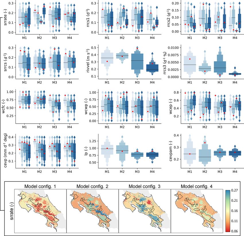
978              S. Arciniega-Esparza et al.: Remote sensing-aided rainfall–runoff modeling in the tropics of Costa Rica

Figure 1. Study area (a) rainfall gauges (blue dots), monitored catchments (red polygons), and sub-basins used in the HYPE model (gray
polygons), (b) soil type at 1 m depth from SoilGrids, where blue polygons correspond to catchments used for rain correction but not for
calibration, (c) major land use categories from CCI Land Cover, (d) precipitation seasonal index with dark blue corresponding to uniform
monthly precipitation and yellow to a more seasonal precipitation regime, (e) mean annual precipitation for the period 1981–2017 from
CHIRPS, and (f) mean annual actual evapotranspiration for the period 2000–2014 from MODIS.

shrubs, grassland, sparse vegetation, croplands). Urban areas         sification was mainly composed of mosaic natural vegeta-
represent less than 0.5 % of Costa Rica. Different CCI LC             tion and croplands (54 % and 13 %, respectively). Finally,
tree categories were grouped into a single tree class, with           the water reclassification consisted of 93 % water bodies and
∼ 87 % corresponding to broadleaved evergreen trees. More             flooded shrub areas.
than 98 % of the reclassified urban areas correspond to the              The climatological space–time series were obtained from
original urban land use from CCI LC. The mosaic reclas-               remote sensing and global products, described in Ta-

Hydrol. Earth Syst. Sci., 26, 975–999, 2022                                              https://doi.org/10.5194/hess-26-975-2022

S. Arciniega-Esparza et al.: Remote sensing-aided rainfall–runoff modeling in the tropics of Costa Rica                                            979

Table 1. Physical and climatological properties of the monitored catchments. Streamflow gauges were grouped according to their location in
the Caribbean and the Pacific basins. AI stands for aridity index and EI stands for evaporative index.

         Zone           Station                Area       Elevation [m a.s.l.]            Slope        Prec        EI      AI            Qt
                                            [km2 ]       Min         Mean        Max       [%]      [mm yr−1 ]                      mean
                                                                                                                                    daily
                                                                                                                                  [m s−1 ]
                        Cariblanco               75     761.7       1850.8       2829.5    26.5       3079        0.44     0.54      9.02
                        Oriente                 229     586.5       1413.7       2740.1    40.1       4202        0.32     0.42     29.90
         Caribbean      Dos Montañas            660     108.5       1316.7       3191.0    37.2       3551        0.36     0.45     53.79
                        Terron Colorado        2061      18.6        734.7       2312.5    21.3       3175        0.44     0.56    149.66
                        Guatuso                 242       7.8        520.6       1881.7    18.9       3968        0.35     0.45     29.38
                        Providencia             122    1365.8       2573.0       3479.7    44.3       2750        0.50     0.68      6.68
                        Tacares                 201     584.3       1404.8       2723.8    17.6       2714        0.49     0.61     11.27
                        Guapinol                210     178.2       1070.4       2173.3    23.7       2879        0.49     0.66     10.13
                        Caracucho              1133      60.9       1251.0       3252.7    24.7       3091        0.43     0.56     72.92
         Pacific
                        El Rey                  656      48.6       1142.1       2501.5    36.5       2648        0.51     0.67     31.96
                        Rancho Rey              320       0.0        490.7       1902.4    15.3       2234        0.57     0.86      9.35
                        Guardia                 961       0.0        336.5       1898.2    11.0       1787        0.68     1.07     23.66
                        Palmar                 4771       0.0       1009.2       3791.0    30.3       3176        0.41     0.55    305.45

Table 2. Remote sensing and global products used in this study.

  Dataset          Variable             Coverage and            Period       Scale        Data type                          Reference
                                        resolution
  CHIRPSv2.0       Precipitation (P )   50◦ S–50◦ N,            1981–        daily        merged remote sensing              Funk et al. (2015)
                                        ∼ 5 km                  present                   interpolated and calibrated
                                                                                          using more than 14 000 rain
                                                                                          gauges
  MOD16            AET and PET          global,                 2000–        monthly      AET and latent heat flux based     Mu et al. (2011)
                                        ∼ 5 km                  2014                      on the Penman–Monteith
                                                                                          equation incorporated remote
                                                                                          sensed MODIS products
  CPC Global       Temperature          89.75◦ S–89.75◦ N,      1979–        daily        gridded temperature from           https://psl.noaa.gov/
  Temperature      (Tmin , Tmax ,       ∼ 50 km                 present                   6000–7000 global stations          (last access:
                   Tmean )                                                                                                   20 November 2020)
  CCI Land         Vegetation cover     global,                 1993–        annual       land cover maps derived from       Bontemps et al.
  Cover            (land use)           0.3 km                  2015                      MERIS remote sensing               (2013)
                                                                                          products and classification
                                                                                          models
  SoilGrids        Silt, sand, and      global,                 –            –            soil properties derived from       Hengl et al. (2017)
                   clay content         0.25 km                                           soil profiles and machine
                                                                                          learning
  SRTM             Land elevation       30 m                    –            –            SAR interferometry                 Bamler (1999)

ble 2. The precipitation grid was obtained from the Cli-                      ranging from 27 ◦ C in coastal regions to 20 ◦ C in the cen-
mate Hazards Group InfraRed Precipitation with Satellite                      tral region at around 1000 m a.s.l. (Esquivel-Hernández et al.,
data (CHIRPS) version 2 (Funk et al., 2015), and the mean                     2017). Figure 1d shows the seasonality of monthly precip-
daily temperature was obtained from the CPC Global Daily                      itation from CHIRPS using the index proposed by Walsh
Temperature product provided by the NOAA/OAR/ESRL                             and Lawler (1981), where lower values (< 0.3) correspond
PSL (https://psl.noaa.gov/, last access: 20 November 2020).                   to a more uniform monthly precipitation, and higher val-
Temperature exhibited low seasonality, with mean values                       ues (> 0.8) indicate that annual precipitation is concentrated

https://doi.org/10.5194/hess-26-975-2022                                                          Hydrol. Earth Syst. Sci., 26, 975–999, 2022
980              S. Arciniega-Esparza et al.: Remote sensing-aided rainfall–runoff modeling in the tropics of Costa Rica

over a few months. Such seasonality is widely controlled            cific). Moreover, the lower AET values overlap with low hu-
by air masses that reach Costa Rica at the Caribbean lit-           midity zones and sparse vegetation areas (northwestern Costa
toral, accumulating more humidity on the Caribbean slope            Rica), as well as higher elevation cloud cover that decreases
(Sáenz and Durán-Quesada, 2015), shown as dark blue ar-             soil evaporation (Caribbean slope mountain region).
eas in Fig. 1d. Meanwhile, the humidity along the Pacific
Basin is highly influenced by the migration of continental air
masses of the Intertropical Convergence Zone (ITCZ), which          3     Materials and methods
establishes the rainy season in May–June and in September–
November (Esquivel-Hernández et al., 2017; Muñoz et al.,            3.1    HYPE model structure and setup
2008).
   The yearly cycle of wet and dry deviations in the ocean–         We used Hydrological Predictions for the Environ-
atmosphere is linked to changes in the sea surface tempera-         ment (HYPE) version 5.9, a semi-distributed hydrological
ture of both the Pacific Ocean and the Caribbean Sea, where         model, for the assessment of water resources and water qual-
the El Niño Southern Oscillation (ENSO) is associated with          ity at small and large scales (Lindström et al., 2010) in order
a decrease of the mean annual precipitation across the Pa-          to simulate the hydrological response of Costa Rican catch-
cific Basin, and an increase of precipitation in the Caribbean      ments. The HYPE model can be considered as the evolution
Basin (Muñoz et al., 2008).                                         of the distributed Hydrologiska Byråns Vattenbalansavdel-
   Moreover, the cold-phase La Niña is the cause of an in-          ning (HBV) model (Lindström et al., 1997). HYPE was de-
crease in precipitation in the Pacific Basin and a decrease in      veloped by the Swedish Meteorological and Hydrological In-
the Caribbean (Waylen et al., 1996). Overall, the mean an-          stitute (SMHI) as the operative model for drought and flood
nual precipitation averaged ∼ 3000 mm for Costa Rica with           forecasting across Sweden (Pechlivanidis et al., 2014). More-
maxima as high as 9000 mm, observed in the headwaters of            over, HYPE was recently applied to other climatic regions
the Reventazón catchment at the northwest of the Talamanca          (Andersson et al., 2017; Arheimer et al., 2018; Berg et al.,
Mountain range and the Caribbean Basin (Fig. 1e). The min-          2018; Lindström, 2016; Pugliese et al., 2018; Tanouchi et al.,
imum annual precipitation of 1200 mm yr−1 is observed on            2019), including a global-scale application (Arheimer et al.,
the northern Pacific Basin in the Bebedero and Tempisque            2020).
catchments.                                                            The HYPE model allows simulating the water balance
   The rainfall patterns across Costa Rica are reflected            and nutrient fluxes at a daily or sub-daily scale using pre-
in the streamflow responses of catchments on the Pacific            cipitation and temperature as forcings (SMHI, 2018). The
and Caribbean sides. The daily streamflow tends to be               model structure (Fig. 2a) describes the major water pathways
higher in the Caribbean Basin (9.2 mm d−1 in comparison             and fluxes, ensuring mass conservation at the catchment and
to 4.2 mm d−1 on the Pacific side, computed from observed           sub-catchment scale. Furthermore, each sub-catchment is di-
streamflow records, Table 1), mainly due to the seasonal cli-       vided into the most fundamental spatial soil and land use
mate across the Pacific slope with reduced water availability       classes (SLCs) depending on the classification of soil types,
during the dry season from December to April. Furthermore,          land cover, climate, and elevation, as shown in Fig. 2b. The
the stream lengths of rivers on the Caribbean slope tend to be      SLCs in HYPE provide the capability to predict streamflows
longer in comparison with rivers from the Pacific Basin (see        in ungauged basins since the parameters that regulate the
the river network in Fig. 1c).                                      fluxes and storages are linked to each SLC, with a maxi-
   Potential evapotranspiration and actual evapotranspira-          mum of three layers of different soil thickness, as shown
tion were obtained from the MODIS product (Mu et al.,               in Fig. 2b. Water bodies such as lakes and rivers may be
2011) distributed by the Numerical Terradynamic Simulation          considered as an SLC, where lakes can be defined as natu-
Group at the University of Montana, USA, which compared             ral lakes or regulated dams with multiple water outputs. For
well to the few available ground stations in Costa Rica, with       full details of the HYPE model, see the description by Lind-
errors from −0.3 to 0.7 mm yr−1 (Esquivel-Hernández et al.,         ström et al. (2010) and the open-access code references lo-
2017). Even though several products of AET and PET are              cated at https://hypeweb.smhi.se/model-water/ (last access:
available at higher temporal resolution (such as GLEAM at           10 June 2021).
a daily time step; Miralles et al., 2011), the spatial resolution      For this study, Costa Rica was divided into 605 catchments
of these products is at least 5 times lower than MODIS (∼           (Fig. 1a) with 12 SLCs obtained from the spatial combi-
5 × 5 km, ∼ 25 km2 ). Since ∼ 70 % of our delimited catch-          nation of soil types and land cover maps shown in Fig. 1b
ments are smaller than 100 km2 , the spatial resolution of the      and c, respectively. Outlet lakes (which discharge to down-
global products plays an important role in capturing the spa-       stream catchments) and internal lakes (which discharge into
tial variability of the water balance for modeling.                 the main river or tributaries) were set up as different SLCs to
   Figure 1f shows the mean annual AET from MODIS,                  consider the water bodies that regulate the streamflow. The
which spatially ranges from 547 to 1612 mm. The highest             largest water body in Costa Rica is the Arenal reservoir, lo-
AET values were observed at the coast (Caribbean and Pa-            cated in the San Carlos River catchment (Fig. 1b). The Are-

Hydrol. Earth Syst. Sci., 26, 975–999, 2022                                           https://doi.org/10.5194/hess-26-975-2022

S. Arciniega-Esparza et al.: Remote sensing-aided rainfall–runoff modeling in the tropics of Costa Rica                                 981

Figure 2. Schematic representation of the HYPE model (a) division into sub-basins and local classes according to topography, land use, and
soil classes and (b) the model structure of Basin 1 considering two main soil–land combinations and lake properties. In (b), the simulated
hydrological processes and variables are shown in black, while parameter names are given in blue. A full description of parameters (in blue)
is available at https://hypeweb.smhi.se/model-water/ (last access: 10 June 2021). The ilake parameter corresponds to an internal lake and the
olake parameter to an outlet lake. T is temperature, P is precipitation, ET is evapotranspiration, Qt is streamflow, and GW is groundwater.

nal reservoir is an artificial lake used for hydropower pur-             uct already incorporates a bias correction procedure but uses
poses with an average surface area of 87.8 km2 and a depth               only a few concentrated ground stations in Costa Rica. The
that ranges from 30 to 60 m. The Arenal reservoir was imple-             performance of CHIRPS estimating annual water balances is
mented as a natural lake since its operational rules are confi-          shown in Fig. S1a and c in the Supplement, with frequent
dential and therefore unknown.                                           underestimation in the monitored catchments. Therefore, we
   Soil thickness varied for different SLCs, with a maximum              applied a linear scaling to further correct for the bias between
soil thickness of 3 m under forests and a minimum of 2 m                 the product and ground precipitation from 75 available sta-
for bare soil cover, following Arheimer et al. (2020). Further-          tions across Costa Rica (Fig. 1a). The corrected precipitation
more, delimited catchments were classified according to their            was estimated as
elevation and location (Pacific Basin and Caribbean Basin),
applying regional factors to correct the hydrological behavior           CHIRPSc (t) = CHIRPS(t) · BF,                                   (1)
of lowland and mountainous catchments with similar SLCs,
resulting in six defined regions.                                        where CHIRPSc is the bias-corrected precipitation at time t,
   Daily time series of precipitation from CHIRPS and tem-               CHIRPS is the original precipitation at time t, and BF is the
perature from NOAA for the period 2000–2014 were ex-                     bias factor. The bias factor was estimated as
tracted for each catchment using GRASS GIS (Neteler et                            µ(P )
al., 2012), where datasets were resampled to 1 km using                  BF =             ,                                              (2)
                                                                                µ(CHIRPS)
the nearest-neighbor criteria and spatially averaged for each
catchment. The climatological forcings were resampled due                where µ(P ) is the mean of the historical precipitation from
to the small size of some catchments (area of ∼ 1 km2 ).                 the ground stations, and µ(CHIRPS) is the mean of the
Arheimer et al. (2020) recommended computing the average                 historical precipitation from CHIRPS. Note that µ(P ) and
of the nearest grids to obtain the forcings instead of deriving          µ(CHIRPS) were computed using the common study period.
the data from the nearest pixel.                                         The simple linear bias correction was preferred over more
                                                                         complex methods due to the lack of a long common period
3.2   Precipitation correction                                           for all stations. Therefore, we used the individual records of
                                                                         more than 60 available stations covering a period from 1980
Rainfall estimations from satellites are subject to systematic           to 2010 to better capture the complex topography and result-
errors that may produce uncertainty in hydrological simula-              ing rainfall patterns.
tions (Goshime et al., 2019; Grillakis et al., 2018; Infante-               Some monitored catchments exhibiting higher annual
Corona et al., 2014; Wörner et al., 2019). The CHIRPS prod-              streamflow than annual precipitation could not be corrected

https://doi.org/10.5194/hess-26-975-2022                                                  Hydrol. Earth Syst. Sci., 26, 975–999, 2022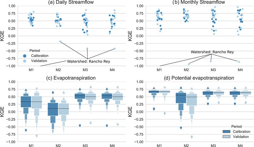
982              S. Arciniega-Esparza et al.: Remote sensing-aided rainfall–runoff modeling in the tropics of Costa Rica

due to groundwater contributions from neighboring catch-           sine function in order to correct the potential evapotranspi-
ments (Genereux and Jordan, 2006; Genereux et al., 2002),          ration (set as zero in this study). To deal with the coarse
under-catch at rainfall gauges (Frumau et al., 2011), and the      spatial resolution of the temperature database (0.5◦ ), a cor-
insufficient number of precipitation stations to correct the       rection factor that depends on catchment elevation was com-
CHIRPS database at a national scale. Nevertheless, errors in       puted (SMHI, 2018):
climatological data have been found to be the most common
issue for water balance modeling in Central America (West-                           tcelevadd · elev
                                                                   tempc = temp −                     ,                         (6)
erberg et al., 2014; Birkel et al., 2012). In that sense, an ad-                           100
ditional approach was implemented to reduce the unrealis-          where tempc is the corrected air temperature (in ◦ C), temp is
tic relationship between streamflow and precipitation, which       the original air temperature (◦ C), tcelevadd is a calibrated pa-
consisted of the creation of virtual stations at the catchment     rameter that corrects temperature (◦ C 100−1 m−1 ), and elev
centroid, where the new bias factor was computed as                is the mean catchment elevation (m). Since only few (<
                                                                 10) temperature station records were available, a bias cor-
         µ Qty + µ AETy
BF2 =                     ,                                 (3)   rection procedure was not possible, but measured tempera-
            µ CHIRPSy                                              ture closely followed the environmental lapse rate (Esquivel-
                                                                   Hernandez et al., 2017). The parameters cevp, cevcorr, cev-
where µ refers to the mean value, Qty is the annual stream-
                                                                   pam, and tcelevadd are part of the Monte Carlo simulation
flow from 1990 to 2003, AETy is the MODIS annual actual
                                                                   and their ranges are shown in Table 3.
evapotranspiration from 2001 to 2014, and CHIRPSy is the
CHIRPS annual precipitation from 1990 to 2014. BF2 adjusts         3.4   Model calibration procedure
the long-term precipitation volume to ensure that the water
balance is preserved, avoiding underestimation of stream-          Figure 3 shows the workflow adopted for model calibration,
flow and evapotranspiration. Four streamflow gauges in addi-       which involves a qualitative parameter sensitivity analysis
tion to those shown in Table 1 were used to cover additional       to find the most suitable range of values for the automatic
spatial area at high elevations for the correction of satellite-   calibration. The initial parameter ranges were obtained from
based precipitation. These streamflow gauges were omitted          manual iterations of one parameter at a time to facilitate au-
from the model calibration–validation procedure due to their       tomatic calibration (Infante-Corona et al., 2014).
shorter records (less than 7 years). The location of the four         We considered four model configurations to analyze the
streamflow gauges and their catchments are shown in Fig. 1b.       effect of including PET and AET in model calibration:
   Finally, BF points from precipitation stations and
BF2 from virtual points were interpolated using the inverse          – model configuration 1 (M1), calibrated using only daily
distance weighted (IDW) method (Shepard, 1968), with an                streamflow (Qt );
exponent value of 2 at the original CHIRPS resolution. The
                                                                     – model configuration 2 (M2), calibrated using monthly
interpolated map of the bias factor was used to spatially cor-
                                                                       streamflow followed by daily streamflow;
rect the time series of CHIRPS across Costa Rica.
                                                                     – model configuration 3 (M3), incorporating a calibration
3.3   Evapotranspiration and temperature correction                    using monthly PET and AET, followed by daily stream-
                                                                       flow;
HYPE incorporates four methods for PET estimation (SMHI,
2018). After initial tests, we found that the monthly PET sig-       – model configuration 4 (M4), similar to M3, additionally
nal from MODIS in Costa Rica can be reproduced by only                 using monthly streamflow before daily streamflow cali-
using temperature as forcing, where PET is computed as                 bration.
PET = (cevp · cseason) · (temp − ttmp) · (1 + cevpcorr) , (4)      For comparison purposes, M1 was chosen as the baseline
                                                                   model configuration, which usually is standard in hydrolog-
where PET is the daily potential evapotranspiration (in mil-       ical practice. The steps are described in Fig. 3. The com-
limeters), temp is the daily mean air temperature (◦ C), cevp is   mon period between Qt and PET-AET is relatively short
an evapotranspiration parameter that depends on the land           (3 years), resulting in Qt and PET-AET calibration using
use (mm ◦ C−1 d−1 ), ttmp is a threshold temperature for evap-     different steps. The automatic calibration consisted of a step-
otranspiration (◦ C), cevpcorr is a correction factor for evap-    wise procedure, where each model configuration was cali-
otranspiration, and cseason is a factor computed as                brated for different fluxes (daily Qt , monthly Qt , monthly

                               2 · π · (dayno − cevpph)
                                                                  AET, monthly PET). The parameter names and initial ranges
cseason = 1 + cevpam · sin                                 , (5)   used for the calibration steps and their configuration are
                                           365
                                                                   shown in Table 3 and Fig. 2. A final step (not shown in Fig. 3)
where cevpam is a correction factor, dayno is the day of the       consisted of calibrating the curve discharge parameters of the
year, and cevpph is a factor used to correct the phase of the      Arenal reservoir using observed water levels. However, the

Hydrol. Earth Syst. Sci., 26, 975–999, 2022                                          https://doi.org/10.5194/hess-26-975-2022
Table 3. Parameter names and initial ranges of the step-wise parameter estimation for each model configuration. Columns M1, M2, M3, and M4 correspond to parameters optimized
during each step of the configuration, and Qt , PET, and AET correspond to the observed time series used to calibrate the model configurations. Qtd means daily streamflow, Qtm monthly
streamflow, PETm monthly potential evapotranspiration, and AETm monthly actual evapotranspiration.
M1 M2 M3 and M4 M3 M4
Model configuration Step 1 Step 1 Step 2 Step 1 Step 2 Step 3 Step 3 Step 4
Random samples 20 000 10 000 10 000 10 000 10 000 10 000 10 000 10 000
Calibration and validation time step day month day month month day month day
Variable for objective function Qt Qt Qt PET AET Qt Qt Qt
Calibration period (YY–YY) 1991–1999 1991–1999 1991–1999 2002–2010 2002–2010 1991–1999 1991–1999 1991–1999
Validation period (YY–YY) 2000–2003 2000–2003 2000–2003 2011–2014 2011–2014 2000–2003 2000–2003 2000–2003
https://doi.org/10.5194/hess-26-975-2022
Type Process Parameter Initial Step 1 Step 1 Step 2 Step 1 Step 2 Step 3 Step 3 Step 4
rage
PET cevpcorr −0.35 to 0 X X X
Regional
Runoff rrcscorr −0.1 to 0.1 X X X X
Runoff srrate 0.01–0.3 X X X X X X
Runoff rrcs1 0.01–0.3 X X X X X X
Baseflow rrcs2 0.001–0.2 X X X X
Percolation mperc1 1–100 X X X
Soil
Percolation mperc2 1–100 X X X
Water content wcfc 0.2–1.0 X X X
Water content wcwp 0.01–1.0 X X X
Water content wcep 0.1–0.8 X X X X X
PET ttmp 1.0–14 X X X X
PET cevp 0.05–0.4 X X X
AET ttrig 0.5–1.5 X X X
Land
AET treda 0.01–1.5 X X X
AET tredb 0.5–15 X X X
Runoff srrcs 0.01–0.3 X X X X X X
AET lp 0.4–1.4 X X X X
PET cevpam 0.15–0.4 X X X
Temperature tcelevadd −0.35 to −0.1 X X X
General
PET epotdist 0.5–2.0 X X X
S. Arciniega-Esparza et al.: Remote sensing-aided rainfall–runoff modeling in the tropics of Costa Rica
Streamflow rivvel 0.1–0.5 X X X X X X
Runoff rrcs3 0.0001–0.01 X X X X X X
Hydrol. Earth Syst. Sci., 26, 975–999, 2022
983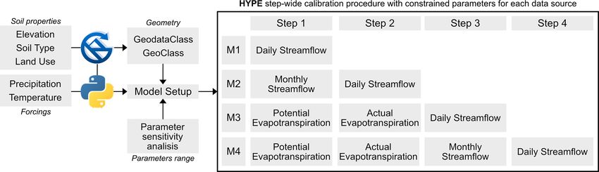
984              S. Arciniega-Esparza et al.: Remote sensing-aided rainfall–runoff modeling in the tropics of Costa Rica

Figure 3. Schematic representation of the HYPE model calibration strategy considering a step-wise procedure to constrain parameters. Four
model configurations (M1, M2, M3, M4) were established using different data sets and/or different timescales. From each calibration step,
the 10th and 90th values of the best-fit parameters were used to constrain the parameters of the next step.

Arenal infrastructure does not contribute to the downstream            3.5   Model calibration and validation using
basins and has a poor impact on the regional model calibra-                  hydrological signatures
tion. Moreover, as previously stated, the reservoir was simu-
lated as a lake since its operational rules are unknown.               The CHIRPS product was evaluated with ground records us-
   The streamflow records were divided into the period                 ing the false alarm rate (FAR, computed with Eq. 7), prob-
from 1991 to 1999 for calibration and from 2000 to 2003                ability of detection (PD, computed with Eq. 8), and threat
for validation. The PET and AET calibration period was es-             score (TS, computed with Eq. 9):
tablished as 2002 to 2010 and the validation period as 2011                       false alarms
to 2014. In both cases, for model warm-up we ran it for                FAR =                      ,                                  (7)
                                                                              hits + false alarms
2 years prior to calibration since our modeling tests showed
                                                                                  hits
that using 2 years was enough to stabilize the effects of initial      PD =                 ,                                        (8)
conditions of water content in soil layers, rivers, and reser-              hits + misses
voirs. The 13 monitored catchments were used for stream-                                  hits
                                                                       TS =                              ,                           (9)
flow calibration. For PET and AET calibration steps, only                   hits + false alarms + misses
the 130 catchments within the 13 monitored catchments were             where hits are days with precipitation detected by CHIRPS
used since our tests showed that using the 605 catchments              and ground rain gauges, false alarms are days where precip-
did not significantly increase the model performance but it            itation was detected only by CHIRPS, and misses are days
did increase the calibration time by a factor of 5. The simula-        where precipitation was detected only by rain gauges.
tions of the 605 catchments were used to compute the metrics              The model performance was evaluated using the Kling–
for the calibration and validations periods.                           Gupta efficiency (KGE; Kling and Gupta, 2009), computed
   A total of 86 parameters were used to build the HYPE                as
model structure consisting of 36 parameters linked to four                         q
soil types, 24 parameters linked to four land cover classes,           KGE = 1 − (r − 1)2 + (∝ −1)2 + (β − 1)2 ,              (10)
6 parameters for the general structure, 12 parameters for the
                                                                                   cov (xo , xs )
regional correction of PET and temperature, and 8 parame-              r = CC =                   ,                                 (11)
ters for lake discharge. The Monte Carlo (MC) routine for pa-                         σo σs
                                                                          σs
rameter sampling and sensitivity analysis included in HYPE             ∝=    ,                                                      (12)
was used for calibration, and the model configurations were               σo
                                                                          µs
run 10 000 times for each step, except for M1, which used              β=    ,                                                      (13)
20 000 runs to cover more parameter combinations since                    µo
this configuration only used daily streamflow. Despite the             where subscripts “o” and “s” correspond to observations and
lower computational efficiency of the MC with respect to               simulations, respectively. µ is the mean, x is the time se-
other optimization schemes (such as gradient-based meth-               ries (streamflow, actual evapotranspiration, or potential evap-
ods), the MC routines are more flexible in accounting for              otranspiration), σ is the standard deviation, r and CC are
multiple parameters sets in complex models (Beven, 2006).              the correlation coefficient, α is the agreement between am-
The 10th and 90th percentiles of the resulting parameters              plitudes, and β is the bias. KGE was chosen as the objec-
from the best 100 runs were used to constrain the parame-              tive function for calibration since it equally captures maxi-
ters for the next calibration step.                                    mum and minimum flows (e.g., Arheimer et al., 2020; Pech-
                                                                       livanidis and Arheimer, 2015; Rajib et al., 2018a; Rakovec
                                                                       et al., 2016; Xiong and Zeng, 2019), and has been described
                                                                       as a relatively balanced metric with slightly more focus on

Hydrol. Earth Syst. Sci., 26, 975–999, 2022                                                https://doi.org/10.5194/hess-26-975-2022
S. Arciniega-Esparza et al.: Remote sensing-aided rainfall–runoff modeling in the tropics of Costa Rica 985
Table 4. Hydrological signatures used as independent performance evaluation criteria.
Signature Equation Description
n
µ = n1
P
Mean.Qtd Qd (i) Mean flow of daily streamflow series
i=1
m = 12 Qd n2 + Qd n+1
Median.Qtd 2 Median value of daily streamflow series
Qd0.33 −Qd0.66
Slope.Qtd slope = 0.66−0.33 Slope of the flow duration curve
CV.Qtd CV = µ(Q d)
σ (Qd ) Variation coefficient, ratio between mean and standard deviation
365
P
N Qd (y,i)
SC SC = N 1 P i=1
Streamflow coefficient, mean of annual streamflow divided by annual precipitation
365
y=1
P
P (y,i)
i=1
365
P
N Qb (y,i)
BFI = N1 i=1
P
BFI 365
Base flow index, mean of annual baseflow divided by annual streamflow
y=1
P
Qd (y,i)
i=1
365
P
N PET(y,i)
AI = N1 i=1
P
AI 365
Aridity index, mean of annual potential evapotranspiration divided by annual precipitation
y=1
P
P (y,i)
i=1
365
P
N AET(y,i)
EI = N1 i=1
P
EI 365
Evaporative index, mean of annual actual evapotranspiration divided by annual precipitation
y=1
P
P (y,i)
i=1
FDC sort (Qd ) Flow duration curve, a plot displaying the statistical distribution of daily streamflow in decreasing order
high flows (Garcia et al., 2017). Non-transformed data were Finally, the non-parametric Kruskal–Wallis (Kruskal and
used given the advice of Santos et al. (2018) against using Wallis, 1952) and Mann–Whitney (Mann and Whitney,
log-transformed discharge with the KGE for low flow eval- 1947) tests were used to detect statistically different perfor-
uation. Furthermore, other statistical criteria were computed mance.
to facilitate assessing the performance of the model config-
urations, such as the Pearson correlation coefficient (com-
puted with Eq. 11), mean absolute error (MAE, computed 4 Results
with Eq. 14), Nash–Sutcliffe efficiency (NSE, computed with
4.1 Remote sensing input data bias correction and
Eq. 15), root mean square logarithmic error (RMSLE, com-
evaluation
puted with Eq. 16), and relative bias (Eq. 17):
n Comparing precipitation from CHIRPS with annual stream-
1X flow and streamflow plus evapotranspiration (assuming long-
MAE = |xs (i) − xo (i)| , (14)
n i=1 term balance P −Qt −AET = 0) showed an underestimation
n of annual precipitation (as shown in Fig. S1a and c), lead-
(xs (i) − xo (i))2
P
ing to unrealistic water balance values. The interpolated bias
i=1
NSE = 1 − n , (15) correction factor (BF, Fig. 4a) showed an overestimation of
P 2 CHIRPS rainfall in blue and underestimations in red. The
(xo (i) − µo )
v
i=1 BF ranged from 0.65 to 1.57 with an average of 1.06 ± 0.14,
u n
uP where the greater disagreements between the ground precipi-
u (log (xs (i)) − log (xo (i)))2 tation and satellite-merged precipitation were observed along
t i=1
RMSLE = , (16) the Pacific Basin. The underestimation reached 30 % to 35 %
n in the north of the Gulf of Nicoya and in the southwest of the
µs − µo Providencia catchment. Underestimation of CHIRPS across
Bias = . (17)
µo the Caribbean slope was mainly observed in the Terron Col-
orado and Cariblanco catchments, with a BF between 1.2
Furthermore, hydrological signatures were calculated to in-
and 1.4. Moreover, the largest overestimation of CHIRPS
dependently assess how well the calibrated model configura-
was observed for the Guanacaste region (BF = 0.65–0.8),
tions reproduced different hydrological criteria. The hydro-
downstream of the Tacares catchment (BF = ∼ 0.8), and to
logical signatures used in this study are shown in Table 4
the southeast of Costa Rica (BF = 0.8–0.85).
and the Budyko curve was constructed from the aridity index
For modeling purposes, we evaluated the temporal syn-
(AI) and evaporative index (EI).
chronicity of rainfall versus streamflow (Fig. 4b) using cross-
https://doi.org/10.5194/hess-26-975-2022 Hydrol. Earth Syst. Sci., 26, 975–999, 2022986 S. Arciniega-Esparza et al.: Remote sensing-aided rainfall–runoff modeling in the tropics of Costa Rica
Figure 4. Performance of the CHIRPS precipitation product in representing observed rainfall in Costa Rica. (a) Interpolated bias factor,
where red areas indicate underestimation and dark blue areas overestimation of CHIRPS with respect to ground stations, and (b) cross
correlations between daily precipitation from CHIRPS and observed daily streamflow, where high correlation values without delay (at zero)
indicate that precipitation and high flows tend to occur on the same day. A high correlation with negative delays indicates that precipitation
occurred on average before the streamflow response.
correlation between daily streamflow and catchment-scale detecting rainy days) for the Pacific Basin (median of ∼ 0.69)
daily precipitation from CHIRPS, where the x axis cor- in comparison with the rain gauges in the Caribbean Basin
responds to the lag time in days. Most of the monitored (median PD of ∼ 0.54). The TS showed similar results to PD
catchments exhibited the highest correlation within lag time (Fig. S2g), with better performance of CHIRPS for the Pa-
zero, indicating that the hydrological response of catchments cific Basin (median of ∼ 0.53) than for the Caribbean Basin
tends to occur within the same day. Nevertheless, the Cari- (median of ∼ 0.46). Such low capacity of CHIRPS to detect
blanco and Rancho Rey catchments exhibited poor correla- rainy days in the Caribbean Basin could affect the perfor-
tion (ρ < 0.3), which means a lack of synchrony between mance of the hydrological model during peak flows.
daily satellite-merged precipitation and streamflow.
The bias correction improved the annual precipitation 4.2 Model performance and parameter uncertainty
where CHIRPSc was consistent with annual streamflow, and
the long-term water balance was mostly preserved, as ob- Figure 5 shows the comparison of the model configura-
served in Fig. S1b and d. Figure S2 shows the MAE normal- tions’ performance for the calibration (dark blue) and vali-
ized by mean precipitation for CHIRPS and bias-corrected dation (light blue) periods. Simulated daily streamflow for
CHIRPS (CHIRPSc), both with respect to the 75 precipi- the 13 gauged catchments was similar for baseline configura-
tation stations, where boxplots correspond to the variabil- tion (M1) and M2 during the calibration period (1991–1999;
ity of normalized MAE estimated by each point. The av- Fig. 5a) with a mean KGE of 0.54±0.09 and 0.53±0.08, re-
erage normalized MAE at a daily scale was estimated at spectively. Nevertheless, M1 showed a median NSE of 0.33
1.2±0.12 mm mm−1 for CHIRPS and 1.17±0.08 mm mm−1 in comparison to M2, which showed a median NSE of 0.25.
for CHIRPSc, 0.30 ± 0.09 and 0.27 ± 0.07 mm mm−1 at a The comparison of the correlation coefficient, median abso-
monthly scale, and 0.16 ± 0.09 and 0.11 ± 0.04 mm mm−1 lute error, and NSE metrics is shown in Fig. S3. Moreover,
at an annual scale, respectively. metrics for M3 and M4 were slightly poorer due to a larger
Figure S2d shows the probability of success and failure dispersion across the sample, with a mean KGE of 0.45±0.2
of CHIRPSc at detecting rainy or dry days with respect to and 0.47 ± 0.17, respectively, and a mean NSE of 0.23 ± 0.2
ground stations, where the probability was computed from a and 0.21 ± 0.21. For the validation period (2000–2003), the
single time series merged from the 75 station records. Fur- mean KGE decreased by ∼ 0.08, but with similar perfor-
thermore, Fig. S2e to g show the false alarm rate (FAR), mance for NSE.
probability of detection (PD), and threat score (TS), respec- The configuration M2 best reproduced monthly stream-
tively. Results indicated that CHIRPSc detected true rainy flow for the calibration period (Fig. 5b), with a mean KGE
and dry days with a similar probability (0.31 to 0.34) as in of 0.67 ± 0.11, whereas the configurations M1, M3, and M4
situ observed rainfall, whereas the FAR ranged from 0.15 showed a mean KGE of ∼ 0.60, also driven by larger dis-
to 0.38 with the greater values (i.e., incorrect detection of dry persion along the KGE scale. The NSE also supports M2 as
days as rainy days by CHIRPS) to the southeast, and the PD the best monthly streamflow predictor for the calibration pe-
showed greater values (i.e., better performance of CHIRPS at riod (Fig. S3), with a median value of 0.54, in contrast to
M1, which showed a median NSE of 0.43. The four model
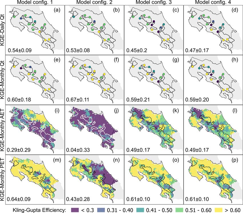
Hydrol. Earth Syst. Sci., 26, 975–999, 2022 https://doi.org/10.5194/hess-26-975-2022S. Arciniega-Esparza et al.: Remote sensing-aided rainfall–runoff modeling in the tropics of Costa Rica 987 Figure 5. The range of KGE values for the calibration (dark blue) and validation periods (light blue). (a) KGE statistical dispersion for daily streamflow, (b) KGE statistical dispersion for monthly streamflow, (c) boxplots of KGE values for AET, and (d) boxplots of KGE for PET. Streamflow calibration period from 1991 to 1999 and validation period from 2000 to 2003. PET and AET calibration period from 2001 to 2010 and validation period from 2011 to 2014. Since the configurations M1 and M2 were calibrated only with streamflow, panels (c) and (d) are for comparison purposes only, showing the effect of including PET and AET in the calibration procedure. configurations preserved performance for the validation pe- the southeast of Costa Rice, such as the Palmar, Caracu- riod, and in some cases, the KGE even increased, as was the cho, El Rey, and Guapinol catchments, with KGEs higher case for the Palmar, Caracucho, and El Rey catchments (not than 0.55 (NSE > 0.4, as shown in Fig. S4) for daily stream- shown). Nevertheless, the Rancho Rey catchment exhibited flow and higher than 0.8 (NSE > 0.63) for monthly stream- poor performance during the validation period (KGE < 0 and flow. Nevertheless, the mid-Pacific Basin also resulted in the NSE < −2) for daily and monthly scales since the four con- Tacares and Providencia catchments exhibiting the worst per- figurations overestimated streamflow. In the following sec- formance for monthly streamflow and the configurations M3 tions, we present more details for Rancho Rey that can ex- and M4 with KGE < 0.3 and NSE < 0 (Fig. 6g and h). plain the catchment behavior and its performance. The spatially distributed KGE on the last two panels Figure 5c and d show the effect of including AET and of Fig. 6 shows the improvement by including AET and PET in the calibration steps, and the KGE was computed by PET in the calibration steps (Fig. 6k, l, o and p), un- aggregating the complete domain (605 nested catchments). like the case of daily and monthly Qt , where no signif- The calibration consisted of 130 nested catchments within icant improvements were observed using the four calibra- the monitored catchments. Furthermore, M1 and M2 were tion procedures. The calibrated monthly AET simulated with only plotted for comparison purposes since these configura- M1 showed low efficiency (KGE < 0.2 and NSE < 0) for tions were calibrated with streamflow. From Fig. 5c, we ob- ∼ 182 catchments of the Pacific Basin but an acceptable served that simulated monthly AET for the calibration pe- performance (KGE > 0.6 and NSE > 0.2) for monthly PET. riod (2002–2010) improved for M3 and M4 with a mean M2 exhibited poor performance across the simulation do- KGE of ∼ 0.49 ± 0.17 with respect to M1 with a mean KGE main for AET and low efficiency of PET in the southeast of 0.29±0.29 and M2 (0.04±0.33). The higher performance Caribbean. Additionally, M3 and M4 showed similar results of AET was also observed for M3 and M4 according to the with acceptable performance (KGE > 0.6 and NSE > 0.2) correlation coefficient and MAE (Fig. S3). Surprisingly, the for ∼ 179 catchments, most of them located in the north- baseline configuration (M1) showed a slightly better per- east. The median MAE and the median correlation coeffi- formance of simulated monthly PET, with a mean KGE of cient for M3 and M4 were ∼ 11 % lower (MAE = ∼ 15 mm) 0.64 ± 0.09, whereas M3 and M4 showed a mean KGE of and ∼ 39 % higher (CC > 0.63) than for M1. Surprisingly, ∼ 0.61 ± 0.10, and M2 a mean KGE of 0.43 ± 0.28 (Fig. 5d). the simulated PET with M3 and M4 was similar to the PET The performance of monthly AET and monthly PET was from M1. The performance of the calibrated water level on similar for the validation period (2011–2014; Fig. S3). the Arenal reservoir was relatively low for all configurations The results from Fig. 6 suggested that the best perfor- (KGE ∼ 0.35, NSE < −0.1, and CC ∼ 0.36), affected by the mance of daily and monthly streamflow for the calibra- unknown quantity of withdrawals from the reservoir during tion period (2001–2009) was obtained for catchments in the driest months (April–July). https://doi.org/10.5194/hess-26-975-2022 Hydrol. Earth Syst. Sci., 26, 975–999, 2022
988              S. Arciniega-Esparza et al.: Remote sensing-aided rainfall–runoff modeling in the tropics of Costa Rica

Figure 6. Matrix of spatially distributed KGE results for the calibration period (streamflow from 1991 to 1999, PET and AET from 2001
to 2010), where green and blue reflect better performance. Configurations M1 and M2 were calibrated only with streamflow. Nevertheless,
PET and AET panels are compared to show the effect of including such variables in the calibration procedure. The mean ± SD of KGE is
shown on the lower left of each panel.

   Figure 7 shows the model parameter ranges from the                 spatial distribution of the srrate parameter, with similar val-
100 best-fit simulations resulting from the last calibration          ues for M2, M3, and M4 and the most frequent soil classes
step for each configuration. The red dots from Fig. 7 cor-            (clay and clay-loam).
respond to the optimal parameters used for modeling, where               The soil parameters that regulate the soil water con-
multiple red dots and boxplots for each model are shown by            tent (wcwp, wcep) showed similar distributions with the me-
soil type and land use.                                               dian value of the fraction of soil water available for evap-
   A large dispersion with a coefficient of variation                 otranspiration (wcfc). The effective porosity (wcep) was
(CV = SD/mean) greater than 0.35 was observed for runoff              slightly higher for configurations M1 and M2, but the final
response parameters (srrate, fraction for surface runoff; srrcs,      parameters (red dots) differed between the models. Further-
recession coefficient for surface runoff) and baseflow param-         more, for M3 and M4, the parameters lp and cevpam exhib-
eters (rrcs1, recession coefficient for uppermost soil layer;         ited constrained distributions with a CV of 0.12 and 0.11,
rrcs2, recession coefficient for lowest soil layer). The impacts      respectively. In comparison, M1 and M2 showed CV values
of monthly streamflow on calibration were observed for the            of ∼ 0.25 and ∼ 0.28 for lp and cevpam.
general model parameters of rivvel (river velocity) and rrcs3
(deep layer recession coefficient), with constrained posterior        4.3   Evaluating streamflow simulations and
parameter distributions for configurations M2 and M4 and                    hydrological signatures
higher velocities and greater baseflow discharge for M2 with
respect to M4.                                                        The step-wise calibration improved model performance in
   The soil type and land use coverage influence the calibra-         different aspects. Figure 8 shows the comparison of the hy-
tions’ parametrization. M2 and M4 showed constrained dis-             drological simulations for two monitored catchments con-
tributions of parameters srrate and rrcs1 for clay-loam soil          trasting the best simulation with the highest KGE perfor-
(third class), the most frequent soil type in the monitored           mance (Palmar catchment) and the worst simulation with the
catchments (Fig. 1b). The bottom panel in Fig. 7 shows the            lowest KGE performance (Rancho Rey catchment).

Hydrol. Earth Syst. Sci., 26, 975–999, 2022                                              https://doi.org/10.5194/hess-26-975-2022
You can also read