Insights into a remote cryosphere: a multi-method approach to assess permafrost occurrence at the Qugaqie basin, western Nyainqêntanglha Range ...
←
→
Page content transcription
If your browser does not render page correctly, please read the page content below
The Cryosphere, 15, 149–168, 2021
https://doi.org/10.5194/tc-15-149-2021
© Author(s) 2021. This work is distributed under
the Creative Commons Attribution 4.0 License.

Insights into a remote cryosphere: a multi-method approach to
assess permafrost occurrence at the Qugaqie basin, western
Nyainqêntanglha Range, Tibetan Plateau
Johannes Buckel1 , Eike Reinosch2 , Andreas Hördt1 , Fan Zhang3 , Björn Riedel2 , Markus Gerke2 , Antje Schwalb4 , and
Roland Mäusbacher5
1 Institute for Geophysics and Extraterrestrial Physics, Technische Universiät Braunschweig,
38106 Braunschweig, Germany
2 Institute for Geodesy and Photogrammetry, Technische Universiät Braunschweig, 38106 Braunschweig, Germany
3 Key Laboratory of Tibetan Environment Changes and Land Surface Processes, Institute of Tibetan Plateau Research,

Chinese Academy of Sciences, Beijing, 100101, China
4 Institute of Geosystems and Bioindication, Technische Universiät Braunschweig, 38106 Braunschweig, Germany
5 Geographical Institute, Friedrich Schiller University of Jena, 07743 Jena, Germany

Correspondence: Johannes Buckel (j.buckel@tu-braunschweig.de)

Received: 22 April 2020 – Discussion started: 2 June 2020
Revised: 26 November 2020 – Accepted: 26 November 2020 – Published: 11 January 2021

Abstract. Permafrost as a climate-sensitive parameter and        in a rock glacier at 5500 m a.s.l. and ice lenses around the
its occurrence and distribution play an important role in the    rock glacier (5450 m a.s.l.). The highest multiannual creep-
observation of global warming. However, field-based per-         ing rates up to 150 mm yr−1 are typically observed on these
mafrost distribution data and information on the subsur-         rock glaciers. This study closes the gap of unknown state of
face ice content in the large area of the southern mountain-     periglacial features and potential permafrost occurrence in a
ous Tibetan Plateau (TP) are very sparse. Existing models        high-elevated basin in the western Nyainqêntanglha Range
based on boreholes and remote sensing approaches suggest         (Tibetan Plateau).
permafrost probabilities for most of the Tibetan mountain
ranges. Field data to validate permafrost models are generally
lacking because access to the mountain regions in extreme al-
titudes is limited. The study provides geomorphological and      1   Introduction
geophysical field data from a north-orientated high-altitude
catchment in the western Nyainqêntanglha Range. A multi-         Information on permafrost (defined as a thermal state of
method approach combines (A) geomorphological mapping,           perennially cryotic ground, frozen for at least 2 consecutive
(B) electrical resistivity tomography (ERT) to identify sub-     years; Ballantyne, 2018; Washburn, 1979) distribution is of
surface ice occurrence and (C) interferometric synthetic aper-   great importance in times of global warming, especially in
ture radar (InSAR) analysis to derive multi-annual creeping      high-mountain areas (Hock et al., 2019), because these ar-
rates. The combination of the resulting data allows an as-       eas are climatically sensitive (Barsch, 1996; Mollaret et al.,
sessment of the lower occurrence of permafrost in a range        2019). The International Panel on Climate Change (IPCC)
of 5350 and 5500 m above sea level (a.s.l.) in the Qugaqie       reported the strongest observed increase in permafrost tem-
basin. Periglacial landforms such as rock glaciers and pro-      perature (globally averaged across polar and high-mountain
talus ramparts are located in the periglacial zone from 5300–    regions) since 2007 in 2019 (Hock et al., 2019). Periglacial
5600 m a.s.l. The altitudinal periglacial landform distribu-     landforms, like rock glaciers and protalus ramparts in this
tion is supported by ERT data detecting ice-rich permafrost      study, are features “resulting from the action of intense frost,
                                                                 often combined with the presence of permafrost” (French,

Published by Copernicus Publications on behalf of the European Geosciences Union.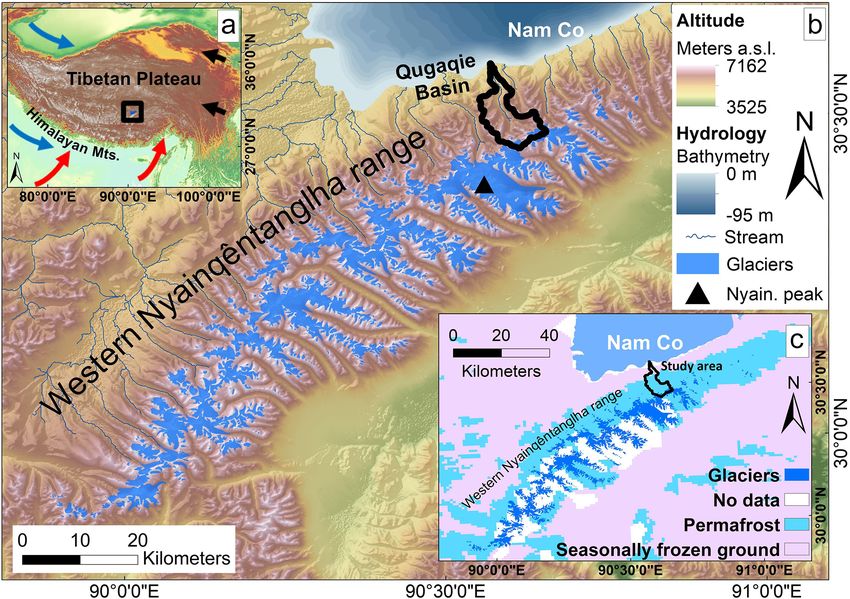
150                                                                        J. Buckel et al.: Insights into a remote cryosphere

2012). If permafrost as perennial frozen ground ice is avail-      tistical and machine learning approaches suggest that the per-
able, periglacial landforms are particularly well suited to de-    mafrost extent on the entire TP is 45.9 % (2003–2010), and
tect and to study changes of permafrost and the related ice        they predict future permafrost degradation of 25.9 % by the
content (Kneisel and Kääb, 2007; Kääb, 2013, Knight et al.,        2040s and 43.9 % by the 2090s (Wang et al., 2019). Cheng
2019). These changes have an increasing impact on people           and Wu (2007) also conclude that more than “half of the per-
and their livelihood (Gruber et al., 2017), e.g., due to the im-   mafrost may become relict and/or even disappear by 2100”.
portance of long-term ground ice as a water resource (Jones           This study aims to supplement the previously summarized
et al., 2019) in arid/semiarid regions like the Andes (Azó-        studies with an assessment of probable occurrence of per-
car and Brenning, 2010; Rangecroft et al., 2016) or the Tien       mafrost in remote high-mountain regions unbiased by the
Shan (Bolch and Marchenko, 2006). The frozen water stor-           location of the Tibetan corridors and to provide a ground
ages have a strong impact on water budgets by permafrost           truthing for existing permafrost studies and maps on the TP.
degradation and glacier melt (Bibi et al., 2018; Song et al.,      The use of the term “probable” is motivated by the fact that
2020), especially at the so-called Asian water tower, which        we do not have ground-truthed temperature data for geophys-
provides water for more than 1.4 billion people (Immerzeel         ical data validation. Furthermore, no small-scaled modelled
et al., 2020). The occurrence of natural hazards increases due     permafrost distribution is available, and therefore we assess
to thawing permafrost (Zhang and Wu, 2012; Yu et al., 2016),       its occurrence indirectly. The spatial heterogeneity of our
for example by destabilizing mountain slopes and rock walls        data (mapping, InSAR and ERT) and of topographic varia-
(Deline et al., 2015). The scientific and social importance        tions in permafrost occurrence also prevents us from provid-
leads to a stronger focus on permafrost areas, especially on       ing precise elevational limits; thus we provide an assessment
the Tibetan Plateau (TP) where permafrost conditions react         of probable occurrence of permafrost in a range according to
fast to atmospheric warming (Cheng and Wu, 2007; Lu et             the findings of the three methods.
al., 2017).                                                           Our study area (Fig. 1b and c) is located at the interface be-
   Permafrost research in engineering has a 60-year-long tra-      tween continuous permafrost and seasonally frozen ground
dition on the TP (Chen et al., 2016; Yang et al., 2010). The       according to large-scale modelling results of permafrost con-
continuous use and life span of infrastructure depends on          ditions on the TP (Sun et al., 2020). The location makes it a
stable surface conditions which are strongly deteriorated by       suitable environment to validate such large-scale models and
permafrost degradation. The engineering corridors for infras-      to precisely define the interface with ground-truthed data.
tructure projects like the Qinghai–Tibetan highway/railway         The validation is important, because the final conclusion
and pipelines (Yang et al., 2010; Yu et al., 2016) were ac-        would be that some higher region on the TP is not completely
companied by monitoring permafrost sites based on bore-            underlying permafrost conditions, unlike expected and mod-
hole temperature (Hu et al., 2020; Li et al., 2009a), ground       elled at other places at the TP (Cao et al., 2019; Ran et al.,
temperature data (Cheng and Wu, 2007; Ma et al., 2006)             2012).
and geophysics: small-scaled ground ice distribution was in-          The identification of periglacial landforms, subsurface
vestigated by ground-penetration radar (Wang et al., 2020;         ice and surface creeping rates on these landforms leads to
Wu et al., 2005; You et al., 2017) and by electrical resistiv-     an assessment of the probable occurrence of permafrost.
ity tomography (ERT) (You et al., 2013, 2017) close to the         The combination of field investigations and remote sens-
important highways/railways. Compared to the central and           ing techniques is a useful tool to detect permafrost occur-
eastern parts of the TP, permafrost surveys in the western         rence (Bolch et al., 2019; Dusik et al., 2015; Monnier et al.,
and southern TP are very scarce (Yang et al., 2010). Addi-         2014). Periglacial landforms such as active (creeping) rock
tional permafrost studies outside the engineering corridors        glaciers and protalus ramparts can contain ice (Barsch, 1996;
are limited to modelling results and large-scale permafrost        Scapozza, 2015; Schrott, 1996) and are considered indicators
distribution maps (Ran et al., 2012; Cao et al., 2019; Obu         of permafrost occurrence (Frauenfelder et al., 1998; Haeberli
et al., 2019). Implications of a temperature warming fol-          et al., 2006; Kneisel and Kääb, 2007; López-Martínez et al.,
lowed by permafrost degradation for the entire TP are hard         2012). Especially on the TP only sparse literature is found
to deduce due to inadequate distribution and a small num-          that describes periglacial landforms in detail in combination
ber of stations recording air temperature (Yang et al., 2010).     with permafrost occurrence (Fort and van Vliet-Lanoe, 2007;
Therefore, modelling approaches are gaining increasing im-         Ran and Liu, 2018; Wang and French, 1995). However, these
portance in order to estimate the consequences of the cur-         periglacial landforms as an indicator for permafrost occur-
rent temperature rise on the TP. This warming temperature          rence are essential for creating large-scale permafrost distri-
trend is reconstructed by δ 18 O records in four spatially well-   bution maps (e.g. Schmid et al., 2015).
distributed ice cores back to the beginning of the last century       We present a multi-method approach to provide a reliable
(Yao et al., 2006). Sun et al. (2020) confirm the relationship     prediction of subsurface ice and permafrost occurrence to an-
between the temperature increase and permafrost degrada-           swer the following research questions:
tion on the TP by a slow adaption until the year 2100 based
on a numerical heat conduction permafrost model. New sta-

The Cryosphere, 15, 149–168, 2021                                                       https://doi.org/10.5194/tc-15-149-2021

J. Buckel et al.: Insights into a remote cryosphere 151
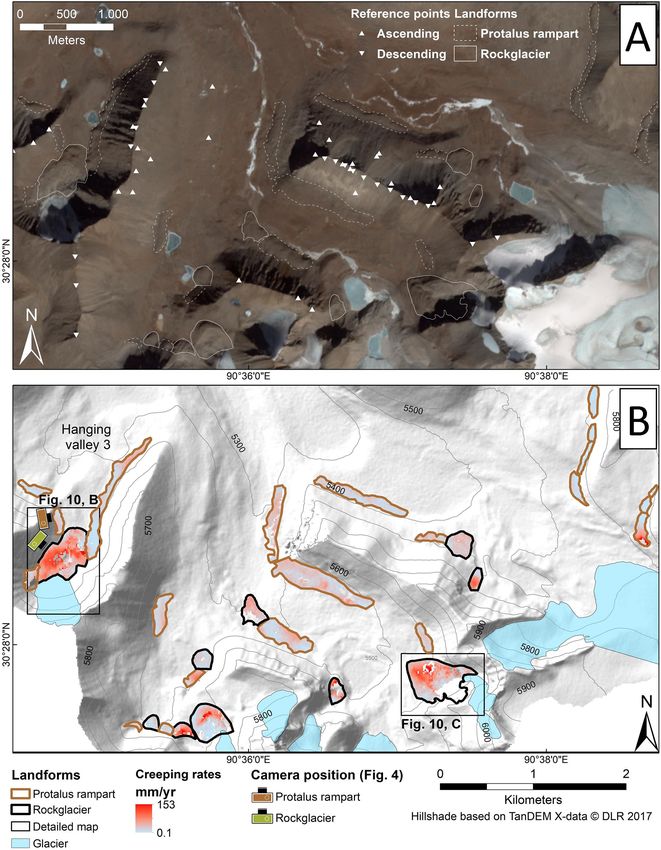
Figure 1. (a) Location of the study area within the Tibetan Plateau (TP) (background on SRTM DEM v4; Jarvis et al., 2008). Different
wind systems influencing climate of the TP are shown by blue (westerlies), red (Indian summer monsoon) and black (East Asian monsoon)
arrows based on Yao et al. (2012). (b) Overview map of the Nam Co catchment with the altitude colours and the study area of the Qugaqie
catchment (thick black lines). Note the greater glacier extents on the south-oriented mountain range. Bathymetric data originated from Wang
et al. (2009) (hillshade and DEM background based on SRTM DEM v4; Jarvis et al., 2008). Glacier extents originated from the GLIMS
database (Cogley et al., 2015; Guo et al., 2015; Liu and Guo, 2014). (c) Permafrost distribution in the western Nyainqêntanglha range based
on Zou et al. (2017).
– How are periglacial landforms distributed? rose violently, forming the Nyainqêntanglha Mountains, with
the highest peak of 7162 m a.s.l. (Kidd et al., 1988; Keil et
– Do the investigated periglacial landforms like rock al., 2010). Our study area, the Qugaqie catchment, is charac-
glaciers and protalus ramparts show an active status? terized by Cretaceous red beds and sandstone in the north-
– Which creeping rates do the periglacial landforms indi- ern part and by early tertiary granodiorites in the centre.
cate? The bedrock of the southern part consists of biotite adamel-
lites and glaciers in the highest zone (Kapp et al., 2005;
We created (A) an inventory of periglacial landforms indi- Yu et al., 2019). The atmospheric circulation pattern and
cating potential subsurface ice occurrence, we (B) acquired the topographic characteristics are responsible for a simi-
electrical resistivity tomography (ERT) data to validate the lar glacier distribution pattern in all north-oriented catch-
ice occurrence of selected landforms and we (C) then used ments of the western Nyainqêntanglha range, including the
multi-annual surface creeping rates from InSAR time series Qugaqie basin (Kang et al., 2009; Bolch et al., 2010). On
analysis to corroborate the hypothesis of long-term ice occur- the lee side of the main western Nyainqêntanglha crest and
rence due to permafrost conditions above a special elevation. therefore at the lee site of the moisture of the Indian summer
As a result, the study provides probable occurrence of per- monsoon (ISM) the glaciers are smaller in area and length
mafrost by combining these three methods for a catchment (Bolch et al., 2010) (Fig. 1b). Bolch et al. (2010) also inves-
in a high-altitude mountain range of the TP. tigated the glacier shrinkage based on satellite data. They ob-
served a glacier retreat of about −9.9 ± 3.1 % between 1976
and 2009. Zhang and Zhang (2017) observe a melting rate
2 Study area −0.30 ± 0.07 m yr−1 over the entire western Nyainqêntan-
glha range from 2000 to 2014. The Zhadang glacier located
The western Nyainqêntanglha Range (Fig. 1) was formed in the Qugaqie head lost an area of almost 0.4 km2 in the
during the Himalayan–Tibetan orogenesis as part of the cen- same time span and covered an area of 2.36 km2 in 2009.
tral Lhasa block (Kapp et al., 2005; Keil et al., 2010). From The corresponding retreat rate is 14 %, slightly larger than
Tertiary to Quaternary, the Nyainqêntanglha area was con- the regional average, which could indicate a slightly faster
trolled and compressed by a fracture belt which folded and
https://doi.org/10.5194/tc-15-149-2021 The Cryosphere, 15, 149–168, 2021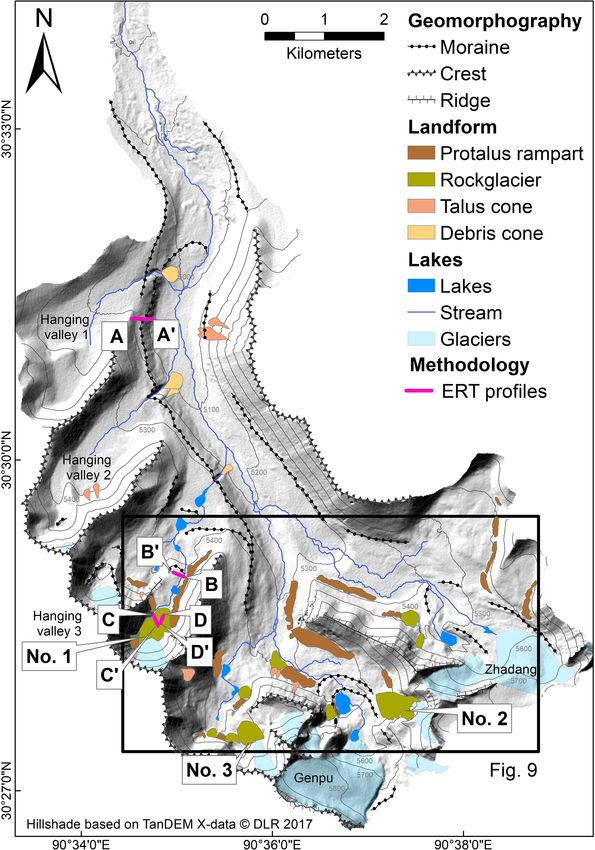
152                                                                          J. Buckel et al.: Insights into a remote cryosphere

deglaciation of the smaller, north-orientated glaciers in the
western Nyainqêntanglha range.
   The Qugaqie catchment is a sub-catchment of the Nam
Co catchment, which is influenced by a strong climate sea-
sonality driven by different wind systems throughout the
year (Yao et al., 2013): westerlies dominate in the winter
months and provide cold, dry continental air from east to
northeast (Fig. 1a, blue arrows), with temperature minima
below −20 ◦ C. The dry season ends with the onset of the
ISM (Fig. 1a, red arrows), which provides moisture from
May to September (Mügler et al., 2010). A total of 80 %
of the annual precipitation (295–550 mm yr−1 ) occurs during         Figure 2. Schematic workflow of applied methods to assess lower
the monsoon-dominated summer months (Wei et al., 2012).              occurrence of probable permafrost.
The influence of the East Asian monsoon on our study area
is minor but it is an important source of moisture for the east-
ern TP (Fig. 1a, black arrows). Consequently, the study area          A. Geomorphological mapping. A map visualizes the dis-
of the Qugaqie basin, situated in the western Nyainqêntan-               tribution and characteristics of periglacial landforms
glha Range (Fig. 1b), is characterized by semiarid climate               and geomorphometric features.
and a large amount of solar radiation due to the high eleva-
tion and reduced cloud cover (Li et al., 2009). With an area          B. Geophysical methods. Electrical resistivity tomography
of almost 60 km2 , the basin drains into the dimictic lake Nam           (ERT) identifies ice content and reveals the subsurface
Co (Fig. 1b), and the relief extends from 4722 m a.s.l. to an            structure of periglacial landforms.
elevation up to 6119 m a.s.l.                                         C. Microwave remote sensing. Interferometric synthetic
   Detailed information about permafrost occurrence and dis-             aperture radar (InSAR) time-series analysis of ESA’s
tribution in the study area is very scarce. Tian et al. (2006) de-       Sentinel-1 satellite data detects perennial, constant
termined a lower limit of permafrost based on soil probes at             creeping rates of active periglacial landforms.
an elevation of around 5400 m a.s.l. along the northern slopes
of Mt. Nyainqêntanglha (Fig. 1b). This is generally higher              (A) A geomorphological map visualizes the distribution
than in other regions (>4500 m a.s.l.) of the TP (Ran et             and characteristics of landforms and geomorphometric fea-
al., 2012). Schütt et al. (2010) sampled lacustrine sediments        tures with the focus on periglacial landforms on a catchment-
from a permafrost lens in an outcrop at the Gangyasang               wide/regional scale. Periglacial landforms like rock glaciers
Qu’s entry into the northwestern end of the lake Nam Co at           (Barsch, 1996) and protalus ramparts (Scapozza, 2015) can
4722 m a.s.l. Zou et al. (2017) distinguish between seasonally       potentially preserve ice over a long period of time (Ballan-
frozen ground and permafrost on their distribution map over          tyne, 2018), and their activity and perennial creeping are an
the TP (Fig. 1c). According to their map permafrost is ex-           indicator for permafrost occurrence (Delaloye et al., 2010;
istent at elevation higher than 5000 m a.s.l. and covers more        Eckerstorfer et al., 2018; Esper Angillieri, 2017). This cir-
than 90 % of the study area. The visible data gaps were not          cumstance is validated (B) by ERT to detect subsurface
further discussed by Zou et al. (2017). A coarse overview            ice on a local scale. (C) InSAR time series analysis de-
including a distinction between glacial and periglacial pro-         tects perennial creeping which is typical of active periglacial
cessual states around the lake Nam Co is given by Keil et            landforms. The permafrost occurrence is indicated by ac-
al. (2010). A 2-year temperature dataset on the Zhadang              tivity of landforms and the corresponding surface struc-
glacier, recorded at 5680 m a.s.l. by an automatic weather sta-      tures like bulges, furrows, ridges or lobes We make use of
tion (2009–2011) at 2 m height, shows a mean annual air tem-         the fact that the deformation of debris supersaturated with
perature (MAAT) of −6.8 ◦ C (Zhang et al., 2013) and sug-            ice causes surface displacement by downwards permafrost
gests permafrost conditions for the surrounding periglacial          creep (Barsch, 1996; Delaloye et al., 2010). Therefore, we
landscape.                                                           concretize surface displacement (rates) as permafrost creep
                                                                     (creeping rates) in this study. Although the continuous move-
                                                                     ment of periglacial landforms and the presence of ice can be
3     Data and methods                                               implied from InSAR data alone, ground truth at selected lo-
                                                                     cations by ERT is essential to exclude other possible inter-
We have used three different methods (A–C) to gain in-
                                                                     pretations.
sights into permafrost-indicating periglacial landforms and
                                                                        We assess the lower occurrence of probable permafrost by
to assess the lower occurrence of probable permafrost in the
                                                                     the mean altitudinal distribution of periglacial landforms, by
Qugaqie catchment. The following methods (Fig. 2) indicate
                                                                     the subsurface ice occurrence which has been validated with
information about permafrost conditions.
                                                                     geophysics and by the active status which is indicated by

The Cryosphere, 15, 149–168, 2021                                                        https://doi.org/10.5194/tc-15-149-2021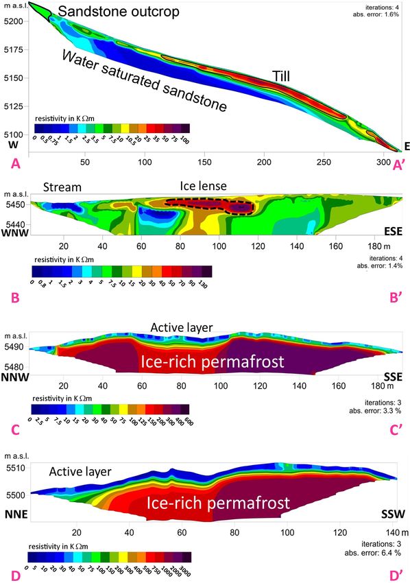
J. Buckel et al.: Insights into a remote cryosphere                                                                               153

                                                                       logical map. During post-mapping we integrated the field-
                                                                       mapped information into ArcGIS. Additional features like a
                                                                       stream network, lakes, ridges, glacier extents and moraines
                                                                       were delineated with the help of the mentioned DEM, a hill-
                                                                       shade map (azimuth 315◦ , altitude 45◦ ) and the mentioned
                                                                       optical images. Glacier extents were digitized based on op-
                                                                       tical images of the year 2013 (BING maps). Rock glaciers
                                                                       were identified following the comprehensive description by
                                                                       Barsch (1996): if the form shows a tongue or a lobate shape
                                                                       in the field and the optical images, we classified the land-
                                                                       form as a rock glacier. Additionally, field observations like
                                                                       coarse clasts at the surface and at the front indicate typi-
                                                                       cal rock glacier substrate. Protalus ramparts are classified
Figure 3. Schematic, hypsometric distribution of mapped land-          by a coarse debris accumulation in front of a rock wall. A
forms. Red features show active, multiannual creeping structures       small depression occurs between the non-lobate bulge and
(furrows, lobes, bulges, ridges) of periglacial landforms indicating   the weathering rock wall. We followed the geomorphologi-
the lower occurrence of probable permafrost. Modified from Barsch      cal mapping approach based on the baseline concepts (V 4.0)
(1996) after Höllermann (1983).                                        of the IPA Action Group “Rock glacier inventories and kine-
                                                                       matics” (Delaloye et al., 2018; Delaloye and Echelard, 2020)
                                                                       and mapped the extended geomorphological footprint of the
perennial surface creeping rates (Fig. 3). An occurrence of            rock glaciers. Additional mapping criteria of rock glaciers
sporadic permafrost is not excluded in lower elevation but             in the field were visible creeping structures on the surface
cannot be validated by the used methods and due to scale               (ridges, furrows and lobes as those shown in Fig. 4a).
issues.                                                                   Protalus ramparts (Fig. 4b) were mapped as periglacial
                                                                       features or permafrost-related landforms as suggested by
3.1   Inventory of cryospheric mesoscale landforms                     Scapozza (2015). A straight headwall for the sediment source
                                                                       is required, as the sediment originated by rockfalls and is
The mapping procedure consists of the elementary map-                  accumulated at the foot of the rock wall. Infiltrating mois-
ping steps, described by Knight et al. (2011) and Otto and             ture originating from precipitation and snowmelt freezes the
Smith (2013). Pre-mapping includes analyses of digital el-             sediment deposit and creates a bulge parallel to the rock
evation models (DEMs) and mapping of landforms on op-                  wall. These ice-permeated rockfall deposits creep down-
tical images at a scale of 1 : 10 000 (named mesoscale here            wards. Scapozza (2015) also noted the challenge to differ-
following Höllermann, 1983). The DEM used in this study                entiate protalus ramparts from initial talus rock glaciers in
originates from TanDEM-X data (2015) with a resolution                 the sense of Barsch (1996). Protalus ramparts mapped in the
of 12 m (© DLR). The optical images are based on Digi-                 present study show no ridges, furrows or lobes at the surface,
tal globe, BING maps (2013) and Google Earth data (2007–               but the mapped rock glaciers do. It is pertinent to point out
2012). Geomorphological symbols were used after Kneisel et             that our mapping procedure both in the field and during post-
al. (1998) for field mapping and after Otto and Dikau (2008)           mapping consistently differentiates between rock glaciers
for the digitized visualization in ArcGIS. During the field            and protalus ramparts based on the above-mentioned crite-
campaign, the main focus was on the mapping of periglacial             ria. An incorrect determination as pronival ramparts can be
landforms at the mesoscale (Höllermann, 1983). These land-             minimized by the absence of longer existing snow fields due
forms are components of the periglacial zone which is de-              to arid climate conditions during the winter and the strong so-
fined by seasonally frozen and perennially frozen ground               lar radiation and less cloud cover due to the extreme altitude
(French, 2017). A differentiation between seasonally frozen            (compare Hedding, 2016).
and perennially frozen movement behaviour is given by the
InSAR data and a derived model by Reinosch et al. (2020).              3.2   Ice detection by ERT
These data were used for the preparation of the cryospheric
landform identification. Next to optical and InSAR data, the           Electrical resistivity tomography (ERT) is a widely used
periglacial landforms were identified in the field by an in-           method in geomorphology (Schrott and Sass, 2008). The ap-
spection of the form, the substrate, the catchment and the             plication works especially well for subsurface ice detection
potential process which formed the landform. The Results               due to strong differences between frozen (high resistivity val-
section describes the inventory statistically and includes mor-        ues) and unfrozen ground (low resistivity values) (Hauck and
phological field observations which could not be included in           Vonder Mühll, 2003; Hauck and Kneisel, 2008). Since the
the map due to scale issues. For example, small-scaled dead            end of the 1990s the method has been established for per-
ice holes were not included in the mesoscale geomorpho-                mafrost detection in solid rock (Krautblatter et al., 2010;

https://doi.org/10.5194/tc-15-149-2021                                                         The Cryosphere, 15, 149–168, 2021
154                                                                               J. Buckel et al.: Insights into a remote cryosphere

Figure 4. (a) Panorama view on a rock glacier (no. 1) with marked creeping structures (lobe in black, ridges in yellow and furrows in dashed
red) in the Qugaqie basin in hanging valley 3. (b) Example of a protalus rampart in hanging valley 3 of the Qugaqie basin. A bulge (in black)
formed through creeping of rockfall deposits. The length of the bulge is approximately 500 m. The location of the photos can be found in
Fig. 6b. (photos: J. Buckel)

Hartmeyer et al., 2012) and in debris–ice mixtures, like rock
glaciers (Von der Mühll et al., 2002; Kneisel et al., 2008;
Rosset et al., 2013; Emmert and Kneisel, 2017; Mewes et al.,
2017).
   For the usual four-point measurement of the ground elec-
trical resistivity, two electrodes feed current into the ground,
which establishes an electric field in the subsurface. Another
pair of electrodes is used to measure the voltage drop be-
tween two other locations on the surface. In order to obtain
                                                                         Figure 5. Measurement setup for the roll-along procedure (adapted
information on the two-dimensional distribution of electri-
                                                                         from N El Sayed et al., 2018).
cal resistivity in the subsurface, a linear arrangement of the
four electrodes is used to measure at different positions along
the profile and with varying distances between the electrodes            ber 2, and so on. The location of the ERT profiles was partly
(Wenner array). The apparent resistivity (m) of each mea-               constrained by logistical conditions. Due to the high altitude,
surement can be calculated from the injected current, the ap-            the crew had to stay at one level for 3 d to get adapted to
plied voltage and a factor, which takes the geometry of the              altitude. The measurement locations were not accessible by
arrangement into account. Subsequently, inverse modelling                vehicles, and a few hours were needed every day to reach the
techniques are used to reconstruct the resistivity structure of          sites, resulting in limited productivity. Therefore, we tried
the subsurface from the measured apparent resistivity data               to locate the profiles efficiently to obtain a representative
(Loke and Barker, 1995).                                                 data set of the valley. We covered different landform features
   We performed ERT measurements during a field campaign                 (moraine, valley bottom, rock glacier) where permafrost con-
in July 2018. We worked with multi-electrode (50) equip-                 ditions were assumed. Blocky surfaces constitute a challenge
ment “GeoTom-MK” (GEOLOG2000, Augsburg, Germany)                         for ERT measurements due to instability and a lack of fine
and a maximum spacing of 2 m, allowing a maximum pro-                    material necessary to provide sufficient contact for the elec-
file length of 98 m with a single measurement. To obtain                 trodes. In cases where no soil material could be found that
longer sections, we used the roll-along procedure illustrated            closed the gaps between the boulders, we inserted the end of
in Fig. 5. For this procedure, two cables were available (de-            each electrode into a sponge saturated with salt water to im-
noted A and B), each equipped with 25 channels. First, both              prove connectivity to the fine material. The saturated sponge
are connected with the control unit to obtain pseudosection              kept the fine material wet and diminished desiccation through
number 1 (Fig. 5). Next, cable B (and all connected elec-                high solar radiation. The ERT data were processed with the
trodes) remains at the same location, whereas cable A is                 Res2Dinv software (© Geotomo Software).
moved to the right of cable B to measure pseudosection num-

The Cryosphere, 15, 149–168, 2021                                                              https://doi.org/10.5194/tc-15-149-2021
J. Buckel et al.: Insights into a remote cryosphere                                                                            155

3.3   Creeping rates by InSAR analyses                             An angle close to 0◦ will cause only minor underestimation,
                                                                   while displacement with a direction near 90◦ to the LOS will
InSAR time series analysis is an active microwave remote           be severely underestimated or even completely overlooked.
sensing technique, which can exploit the phase change of           The Sentinel-1 satellites follow a circumpolar orbit and ob-
the backscattered microwaves to determine relative surface         serve the Earth obliquely with an incidence angle of 33–
displacement on the order of millimetres to centimetres (Os-       43◦ (Yague-Martinez et al., 2016). Both ascending (satellite
manoğlu et al., 2016). Both the amplitude and the phase of        travelling south to north) and descending (satellite travelling
the microwave backscatters are used for InSAR. After pre-          north to south) acquisitions are therefore sensitive to vertical
cisely co-registering all acquisitions, it is possible to calcu-   surface displacement and towards the east or west but very
late the average phase change of each resolution cell over         insensitive to displacement towards the north or south. We
time, which contains a number of different signals, includ-        always select the geometry with the highest sensitivity to-
ing whether a resolution cell moved closer to the receiver,        wards the expected displacement direction to calculate our
i.e. the satellite, or further away from it. These images of       displacement and velocity results.
phase change are called interferograms. The accuracy of the           The surface displacement data presented in this study rep-
derived motion is dependent on a number of different factors,      resent a spatial subset of a surface displacement model origi-
including the frequency of the emitted wave, the atmospheric       nally based on Reinosch et al. (2020). For our analysis of the
delay, the accuracy of its modelling, the topographic data         Qugaqie basin, we processed 278 interferograms from 74 as-
used to correct the images, the choice of reference points,        cending acquisitions (June 2015 to December 2018) and 257
the surface characteristics of the observed structure and the      interferograms from 63 descending acquisitions (November
frequency of the data acquisitions (Hu et al., 2014).              2015 to December 2018) (Table 1). The temporal baselines,
   The reliability of an interferogram is often described by its   i.e. the time period between two data acquisitions, of indi-
so-called coherence. Coherence is a measure of phase stabil-       vidual interferograms is mostly 12 to 36 d with a maximum
ity with a value near zero representing poor reliability and       of 72 and 96 d for ascending and descending orbits respec-
values near 1 representing high reliability (Crosetto et al.,      tively. All data acquisitions originate from ESA’s Sentinel-
2016). If the backscatter characteristics of the observed sur-     1A/B satellite constellation. Both ascending and descending
face change too much between two acquisitions, e.g. due to         datasets were processed using small baseline subset (SBAS)
snow cover, vegetation or events occurring between the ac-         time series analysis (Berardino et al., 2002), with a coherence
quisitions like rockfalls, the coherence is poor and no phase      threshold of 0.3. Mean velocities were calculated by dividing
change can be determined reliably. Coherence also decreases        the cumulative displacement observed during the observation
with increasing displacement, and displacements larger than        period by the length of the observation period (2015–2018).
half the SAR wavelength (∼ 2.8 cm for Sentinel-1) cannot be           All surface velocity data of periglacial landforms have
determined accurately. For this study we chose a coherence         been projected along the direction of the steepest slope under
threshold of 0.3 and discarded areas with coherence values         the assumption that the motion of the described landforms
below 0.3. This threshold is similar to the one chosen by          is mainly gravity-driven by an ice–debris mixture. Hereafter
Sowter et al. (2013) and provides good spatial data cover-         we will refer to the mean surface velocity of periglacial land-
age while also excluding unreliable data. The issue of low         forms projected along the steepest slope as “creeping rates”
coherence or decorrelation is exacerbated for interferograms       to reflect this assumption. We calculate a sensitivity coeffi-
with a long temporal baseline, i.e. a long time period between     cient to compensate for the underestimation of the displace-
data acquisitions. No Sentinel-1 data are available for a pe-      ment signal caused by the disparity between the LOS and the
riod of 48 to 96 d during the summers of 2016 and 2017.            assumed displacement direction. We followed an approach
These longer temporal baselines cause decorrelation during         developed for the study of landslides (Notti et al., 2014), as
the summer months on some of the faster landforms. Freez-          the displacement of landslides is gravity-driven, which we
ing and thawing of the ground leads to reduced coherence           also assume to be true for the periglacial landforms inves-
values in autumn and spring. The coherence over periglacial        tigated in this study. Creeping rates presented in this study
landforms in the Qugaqie basin is relatively good, due to the      were not verified by independent measurements (GPS mea-
lack of high vegetation on actively moving landforms and           surements, laser scans, optical remote sensing, etc.), as no
the relatively sparse snow cover in winter visible on optical      such data sets exist for our study area. Reference points are
Sentinel-2 acquisitions.                                           located on bedrock whenever possible and on ridges or sta-
   Exploiting the phase change with InSAR provides only            ble, vegetated moraines with good coherence if no coher-
relative surface motion towards the satellite or away from it.     ent bedrock was available (compare Fig. 9a). Areas which
The line of sight (LOS) of the satellite is therefore very im-     are likely unmoving on a multiannual scale, such as the old
portant, as motion with a very different direction compared        moraines at the entrance of the Qugaqie basin, display LOS
to this LOS is severely underestimated (Hu et al., 2014). The      velocities of ±2.4 mm yr−1 during our observation period.
severity of this underestimation depends on the angle be-          This does not provide information regarding the accuracy of
tween the LOS and the direction of the surface displacement.       the seasonal variations in our surface displacement results but

https://doi.org/10.5194/tc-15-149-2021                                                     The Cryosphere, 15, 149–168, 2021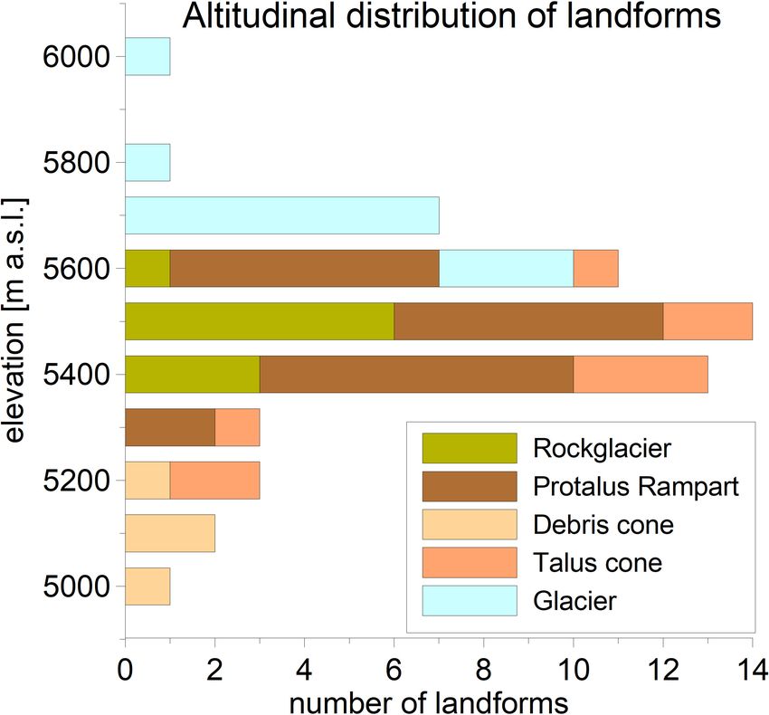
156                                                                           J. Buckel et al.: Insights into a remote cryosphere

Table 1. Summary of ISBAS processing parameters.

          Geometry        Observation period       Acquisitions    Interferograms   Temporal baseline     Coherence threshold
          Ascending    2015-06-05 to 2018-12-22         74              278             12 to 72 d                0.3
          Descending   2015-11-15 to 2018-12-29         63              257             12 to 96 d                0.3

it indicates that the multiannual LOS velocity results are re-
liable. We use this variation of ±2.4 mm yr−1 over likely sta-
ble areas as the precision of the mean LOS velocity during
our observation period. The precision of the creeping rates
was determined by dividing the precision of the LOS veloc-
ity by the sensitivity coefficient. It therefore varies between
2.4 and 12.0 mm yr−1 for areas with a sensitivity coefficient
of 1 and 0.2 (Reinosch et al., 2020).

4     Results and interpretation

4.1    The cryosphere of the Qugaqie basin

The geomorphological map in Fig. 6 shows features of
the mesoscale cryosphere in the Qugaqie basin: glaciers,
moraines, protalus ramparts and rock glaciers. The moraine
distribution suggests that former glaciers extended to the
present shoreline of the Nam Co at their largest size during
Marine Isotope Stage (MIS) 3 (Dong et al., 2014). Multi-
ple smaller moraines are displayed in closer proximity to to-
day’s glaciers (Fig. 6). Glacial landforms like valley glaciers,
cirque and wall glaciers increase in number and size towards
the south due to a higher elevation and shorter distance to
the main ridge (Fig. 6). Only the Genpu (1.56 km2 ) and the
Zhadang (1.41 km2 ) glaciers are considered valley glaciers;
most of the other glaciers are located in the head of the hang-
ing valleys as cirque glaciers. The northward orientation of
all glaciers is a result of the lee effect towards incoming
                                                                     Figure 6. Geomorphological map of the Qugaqie basin. The loca-
moisture from the southern direction. The topographic bar-
                                                                     tions of the ERT profiles are shown with purple lines. Periglacial
rier of the western Nyainqêntanglha Range detains precipita-
                                                                     landforms are greenish (rock glaciers and protalus ramparts). The
tion and causes an asymmetric and uneven north–south dis-            black rectangle represents the boundary of the map shown in Fig. 9.
tribution of glacier extents expressed by smaller extents in
the northern catchments draining in the Nam Co like Qugaqie
(compare Bolch et al., 2010). The glacial zone with a cu-
mulative glacier area of 4.07 km2 (Bing maps, 2013) extends          dating ice occurrence and the status of activity of these land-
from 5500 m a.s.l. to the highest elevation (6086 m a.s.l.) with     forms.
a mean elevation of 5770 m a.s.l.                                       Most rock glaciers are located in cirques, and three are
   The altitudinal (mean) landform distribution illustrates the      supplied by glacial meltwater resulting in greater extents
statistical analyses and displays a typical high-mountain pat-       compared to rock glaciers without a glacier in their catch-
tern (Fig. 7). Debris and talus cones can be found in lower al-      ment (Fig. 6, nos. 1, 2 and 3). Additionally, moraine deposits,
titudes. The periglacial landforms (i.e. protalus ramparts and       talus slopes and protalus ramparts provide the sediment ac-
rock glaciers) are located between elevations of 5300 and            cumulation at the base required for the formation of a rock
5600 m a.s.l., and the average number of periglacial land-           glacier besides water availability (Knight et al., 2019). The
forms is situated around 5500 m a.s.l. We conclude from this         altitudinal distribution of the rock glaciers extends from 5363
altitudinal distribution a probable occurrence of permafrost         to 5789 m a.s.l. with a mean elevation around 5500 m a.s.l.
higher than 5300 m a.s.l., which has to be supported by vali-        (Fig. 7, Table 2). Rock glacier surfaces display clear creep

The Cryosphere, 15, 149–168, 2021                                                          https://doi.org/10.5194/tc-15-149-2021
J. Buckel et al.: Insights into a remote cryosphere                                                                             157

                                                                    terms of material characteristics. Different studies show re-
                                                                    sistivity values of till in a range from 1 to 10 km (Reynolds,
                                                                    2011), from 5 to 10 km (Thompson et al., 2017) and from
                                                                    50 to 100 km (Vanhala et al., 2009). The diversity of resis-
                                                                    tivity ranges and the resulting non-uniqueness can be over-
                                                                    come by using additional methods to support the final con-
                                                                    clusions.
                                                                       Profile A (Fig. 8) ranges from 5090 to 5230 m and rep-
                                                                    resents subsurface conditions in the lower altitudinal areas
                                                                    of the catchment, for example in a lateral moraine. At the
                                                                    surface the profile has a length of 348 m, but the length in-
                                                                    formation in the following text refers to the x axis which
                                                                    corresponds to planar 2D view (the topographic effect is not
                                                                    displayed). From ∼ 120 m on, we observe a slope-parallel,
                                                                    highly resistive layer (highlighted by the black line in Fig. 8a)
                                                                    with resistivity values ranging between 5 and 100 km and
Figure 7. Altitudinal (mean) landform distribution of the Qugaqie
                                                                    an average thickness of 10 m. We interpret this layer as com-
basin derived from the landform inventory.                          pressed till without ice content, based on the resistivity range,
                                                                    the compressed glacial sediment accumulation and the ab-
                                                                    sence of creeping structures indicating ice. According to Yu
structures and rock-glacier-typical bulges, furrows and lobes       et al. (2019) the underlying bedrock consists of sandstone,
(Fig. 4a). There is no pronounced lichen growth, and the            which explains the low resistivity values below the resistive
uppermost material is extremely unstable. These field ob-           moraine deposits. Between 0 and 20 m along the profile, the
servations in combination with the observed creeping rates          electrodes were directly attached to the outcropping, weath-
(Fig. 9b) allow the conclusion of an active status of the rock      ered sandstone. The resistivity values around 5 km corre-
glaciers, which indicates ice occurrence and, thus, permafrost      spond to dry sandstone bedrock, which is exposed to strong
conditions (according to Barsch, 1996). The altitudinal distri-     solar radiation. The hydraulically impermeable till cover is
bution of protalus ramparts has a narrower range of min–max         not present between 20 and 120 m, and moisture infiltrates as
values, but they are located at a similar mean elevation. The       slope water saturating the sandstone bedrock underneath the
mean area of the individual protalus ramparts is only half          moraine and decreasing electrical resistivity.
of the mean area of the individual rock glaciers, i.e., pro-           Profile B (Fig. 8b) is located in hanging valley 3 on top of
talus ramparts are generally smaller than rock glaciers (Ta-        an old, terminal moraine crossing the stream, which drains
ble 2, Fig. 6), but there are twice as many. Protalus ramparts      the hanging valley (Fig. 6). Surrounding dead ice holes in-
are situated in front of rocky slopes and are characterized in      dicate former subsurface ice occurrence behind the former
contrast to rock glaciers by a shorter dimension downslope          moraine terminus. Complete vegetation cover of compresia
(Figs. 4 and 6).                                                    pygmea interspersed with individual rockstones suggests an
   The mesoscale periglacial landforms (mean elevation) are         old and stable surface. From the high resistivity anomalies
situated between 5300 and 5600 m a.s.l. This altitudinal dis-       of up to 150 km, we conclude that ice-poor permafrost in
tribution serves as one component of the three methods for          contrast to ice-rich permafrost in profiles C and D is present
assessing the probable occurrence of permafrost in the catch-       as an ice lens at 5450 m a.s.l.
ment.                                                                  Profiles C and D (possibly the highest-elevated ERT mea-
                                                                    surements worldwide) show the typical two-layer structure
4.2   ERT-based ice detection                                       of rock glacier no. 1 with equally high resistivity values
                                                                    (Fig. 8c, d). The first layer is characterized by lower re-
ERT is a common method to detect ground ice in the sub-             sistivity values (1–20 km), indicating the unfrozen active
surface, inferring permafrost conditions (Lewkowicz et al.,         layer during the summer months. The active layer thickness
2011), if ground ice is present for 2 consecutive years. With       varies between 2 and 5 m. The second layer shows high re-
the help of ERT we were able to provide evidence for the            sistivity values of up to 3500 km and covers the complete
existence of ground ice at specific test sites. Figure 6 dis-       section from below the active layer to the maximum depth
plays the locations and indicates an altitudinal increase in the    of investigation. No internal heterogeneities are visible due
four ERT profiles (A to D). The measured resistivity values         to the lack of current flow within this highly resistive unit,
were compared with tables by Hauck and Kneisel (2008) and           which we interpret as a mixture of ice and sediment. Accord-
Mewes et al. (2017). These studies also address ice detection       ing to Table 3, we interpret the second layer to be ice-rich
in high-altitude periglacial environments. Table 3 sums up          permafrost. Similar resistivity values of ice-rich rock glacier
our measured resistivity values and classifies the values in        material, reaching maximum values of 1000 k,m have been

https://doi.org/10.5194/tc-15-149-2021                                                       The Cryosphere, 15, 149–168, 2021
158 J. Buckel et al.: Insights into a remote cryosphere
Table 2. Statistical description of cryotic landforms based on DEM analyses.
No. Cumulative Area Elevation Elevation
area [m2 ] (mean) (min, max) (mean)
Protalus rampart 22 1 018 014 46 273 5292, 5685 5530
Rock glacier 10 830 185 83 019 5363, 5789 5523
Glacier 11 4 075 580 370 507 5504, 6086 5771
Figure 8. Electrical resistivity sections along the four ERT profiles recorded in July 2018 with a standard spacing of 2 m. Profiles C and D
are located on rock glacier no. 1. Note the increasing elevation between profiles A and D.
reported in several studies from Häberli and Vonder Mühll The relatively large altitudinal steps between our four ERT
(1996), Vanhala et al. (2009), and Mewes et al. (2017). Pro- profiles do not allow exclusion of the occurrence of subsur-
files C and D confirm the presence of subsurface ice at an face ice in other, lower parts of the valley. Therefore, we use
elevation around 5500 m a.s.l., which we use as evidence for the following perennial creeping rates to exclude this case.
the lower occurrence of probable permafrost. The detection of subsurface ice is the second component of
the three methods for estimating the probable occurrence of
The Cryosphere, 15, 149–168, 2021 https://doi.org/10.5194/tc-15-149-2021J. Buckel et al.: Insights into a remote cryosphere 159
Figure 9. (a) Sentinel-2 satellite image, recorded 30 January 2018. Triangles indicate stable reference points. Dashed lines indicate the
outlines of the periglacial landforms. (b) Creeping rates from periglacial landforms move in the slope direction over the observation period
2015–2018. The black rectangles mark the location of the two fastest rock glaciers in Fig. 10. The camera positions correspond to the
photographs in Fig. 4.
permafrost. Inferred by ERT data, subsurface ice can be ex- 96 d for ascending and descending data respectively. Long
pected at selected locations from an altitude of 5450 m and temporal baselines on relatively fast moving landforms may
higher. lead to aliasing effects if the displacement exceeds a quarter
of the wavelength of the satellite (Crosetto et al., 2016). This
4.3 Creeping rates of periglacial landforms would correspond to a LOS displacement of ∼ 14 mm for
Sentinel-1, which emits a wavelength of 56 mm. A total of
The creeping rates for rock glaciers and protalus ramparts, 14 mm in 72 d or 96 d corresponds to a LOS velocity of ap-
including statistical information, are shown in Table 4. The proximately 71 mm yr−1 for ascending and 53 mm yr−1 for
fastest moving areas of landforms display lower coherence descending data. Displacement values in areas with higher
values and small spatial data gaps. The low coherence values LOS velocities than these thresholds are likely to be under-
in those areas are likely connected to the long temporal base- estimated with the InSAR technique and display poor coher-
lines of interferograms in summer of 2016 of up to 72 and
https://doi.org/10.5194/tc-15-149-2021 The Cryosphere, 15, 149–168, 2021160 J. Buckel et al.: Insights into a remote cryosphere
Table 3. Resistivity values for different materials derived by field glaciers’ surface corroborate the mapped landforms’ classi-
measurement. The used terms of the interpreted material followed fication and indicate activity of the landform. By integrat-
Hauck and Kneisel (2008) and Mewes et al. (2017). ing the ERT results of detected subsurface ice occurrence, a
further component of the permafrost condition (subsurface
Material Resistivity below 0◦ ) is validated. Completing the permafrost definition
[km]
(of 2 or more consecutive years) the derived creeping rates by
Sandstone (moist–dry) 0.5–5 InSAR show a constant motion of more than 2 years, which
Till 20– 80 is attributed to the deformation of the debris ice matrix of
Unfrozen sediment (moist–dry) 1–20 the periglacial landforms. So, the active status, the altitudi-
Ice-poor permafrost (ice lenses, ice-interspersed till) 50–150
nal distribution of the periglacial landforms and validated ice
Ice-rich permafrost (massive ice body) 150–4000
occurrence by ERT suggest a lower limit of probable per-
mafrost between 5300–5450 m a.s.l. This range includes ice
lenses detected by ERT data as well as all creeping land-
ence values near or below the coherence threshold of 0.3. forms, indicating an active status and therefore an existence
Coherence values do not drop significantly in winter, which of ice.
is likely due to the semiarid climate and therefore relatively
thin snow cover.
Protalus ramparts in the Qugaqie basin display lower av- 5 Discussion
erage surface velocities than rock glaciers. The creeping rate
of protalus ramparts (11.0 mm yr−1 with an uncertainty from One critical issue for the estimation of the lower occurrence
6.8 to 16.7) is lower and shows more pronounced seasonal of probable permafrost by the used approach is the focus
variations than on rock glaciers (21.1 mm yr−1 with an un- on periglacial landforms. These landforms are characterized
certainty from 11.6 to 36.8). Rock glacier no. 1 of hanging by blocky material and a special thermal regime that low-
valley 3, which we also studied with ERT measurement, dis- ers the internal temperature in comparison to the thermal
plays creeping rates of up to 70 mm yr−1 in most areas, with regime outside of the blocky, rough surface (Gorbunov et
the fastest moving part reaching 153 mm yr−1 (Fig. 10b), al., 2004). This cooling effect of high-porosity, unconsol-
similar to rock glacier no. 2 (Fig. 10c). A time series of creep- idated debris is especially observed in lower mountain re-
ing rates of rock glacier no. 1 is shown in Fig. 10a (black line) gions by near-surface ground temperature measurements on
and of rock glacier no. 2 in Fig. 10a (grey line). The spatial rock glaciers (Onaca et al., 2020) and suggests a lowering
distribution of the creeping rates is relatively uniform in ar- of discontinuous and sporadic permafrost occurrence (Lam-
eas with good InSAR sensitivity, i.e. slopes with an east or biel and Pieracci, 2008; Otto et al., 2012). By using the ERT
west aspect, but displays significantly higher noise level in method we found ice-poor permafrost in ice lenses in min-
areas with poor InSAR sensitivity, i.e. slopes with a north or eral soils next to the rock glacier that corroborates the idea
south aspect. of permafrost conditions outside of blocky material at an el-
We do not observe a clear correlation between variations evation of 5450 m a.s.l. The extreme cold mean annual air
in creeping rates and possible seasonal forcing mechanisms temperature of −6.8 ◦ C at 5680 m a.s.l. (Zhang et al., 2013)
such as temperature or precipitation. Neither protalus ram- should minimize the effect of different regolith properties
parts nor rock glaciers display clear acceleration of creeping that favours permafrost conditions.
in summer compared to winter (Fig. 10a). The next critical issue for the estimation of the lower oc-
The third component for assessing the occurrence of per- currence of probable permafrost is the question of whether
mafrost is based on the movement rates of periglacial land- the huge resistivities observed on profile A (Fig. 8a, black
forms. Based on the assumption that a measurable movement lines) indicate ice or not. In general, subsurface material
rate is determined by perennial ice in the subsurface, the ob- determination without additional cross-validating techniques
served active status of the periglacial landforms allows the by other geophysical methods or borehole data remains un-
conclusion of permafrost occurrence in the corresponding certain (Hauck and Kneisel, 2008; Guglielmin et al., 2018).
landform. Therefore, the geomorphological knowledge of the study
area is essential for an interpretation of the subsurface: in this
4.4 Assessment of the lower permafrost limit of the case, the measured resistivity values of profile A (Fig. 8) of
Qugaqie valley up to 100 km are consistent with both till and ice-poor per-
mafrost (Schrott and Sass, 2008). From the resistivity values
The assessment of the lower permafrost limit consists of it is therefore not possible to determine whether the till con-
an integration of different results. The field-based mapping tains ice or not. However, field observations allow the conclu-
of periglacial landforms indicates the first precondition to sion that no ice was measured because clear creep structures
find permafrost conditions. Field observations like furrows, would have to be recognizable due to a significant slope. Fur-
ridges, coarse substrate and lichen coverage on the rock thermore, InSAR analysis of this location shows no clear
The Cryosphere, 15, 149–168, 2021 https://doi.org/10.5194/tc-15-149-2021J. Buckel et al.: Insights into a remote cryosphere 161
Table 4. Summary of InSAR-derived creeping rates for the periglacial landforms. The values represent the median of all data points over
the entire observation period (2015–2018) on the respective landform. Uncertainty is given by the interquartile range in round brackets.
The percentage of interpolated time periods describes how many interferograms are incoherent and therefore require interpolation with the
ISBAS algorithm.
Landform Creeping rate Summer Creeping rate Coherence Interpolated Data
[mm yr−1 ] acceleration [%] precision [mm yr−1 ] time period [%] points
Protalus ramparts 11.0 (6.8 to 16.7) −2 (−36 to 36) 5.2 (3.9 to 7.8) 0.74 (0.70 to 0.80) 2.5 (0.7 to 6.2) 7984
Rock glaciers 21.1 (11.6 to 36.8) −23 (−46 to 3) 5.1 (4.2 to 8.1) 0.66 (0.59 to 0.73) 7.9 (3.8 to 13.0) 5402
Figure 10. (a) Summer months with air temperatures >0 ◦ C (according to Zhang et al., 2013) are shown in red. Time series represent the
moving average of the 10 nearest values in time based on the median of time series points, located in (b) (black dots) and (c) (grey dots). The
black time series (rock glacier no. 1 in b) is based on ascending data and the grey time series (rock glacier no. 2 in c) on descending data.
perennial creep behaviour (Reinosch et al., 2020), making the extremely difficult logistical constraints in this remote lo-
the presence of subsurface ice unlikely. In order to uniquely cation, these methods could not be applied, and we thus rely
identify ice, it would have been desirable to apply additional on combining evidence from field observations with geo-
geophysical methods, like ground-penetrating radar, refrac- physical results.
tion seismic tomography or capacitively coupled resistivity The approach by Kneisel and Kääb (2007) uses a simi-
(Mudler et al., 2019). In particular, the combination of elec- lar combination of methods as used in this study to describe
trical and seismic methods allows the derivation of a petro- periglacial morphodynamics of a glacier forefield including a
physical four-phase model (Hauck et al., 2008; Mewes et al., rock glacier. ERT profiles show the same range of layer thick-
2017) and the estimation of the sediment-to-ice ratios from ness of 2–5 m as in our profiles in the summer months. They
electrical resistivity and seismic velocities. However, due to recommend the joint application of geoelectrical and surface-
https://doi.org/10.5194/tc-15-149-2021 The Cryosphere, 15, 149–168, 2021162 J. Buckel et al.: Insights into a remote cryosphere
movement data to investigate periglacial landforms and to as- pronounced the lower the mean annual air temperatures and
sess the permafrost distribution, because the combination of the shorter the time spans of positive air temperature are. It
both tools allows a more comprehensive characterization of seems that the magnitude of seasonal variations in the creep-
permafrost characteristics like ice-rich or ice-poor. Also, in ing rates also decreases with a lower availability of moisture,
our case, we believe the ground-based geophysical surveys because the strongest seasonality is observed in moist regions
are useful, as predicting subsurface ice content and deriving such as the Alps. Additionally, catchments in the Qugaqie
permafrost distribution maps only by modelling and/or using basin are quite small for sediment release, so the extent of our
remote sensing includes various sources of error. rock glaciers is limited by a small debris input. Probably for
similar reasons, protalus ramparts investigated in this study
– Low resolution (1 km gridded) of the permafrost-
creep with a median velocity of 11 mm yr−1 , while compara-
distribution models over the entire TP (Zou et al., 2017;
ble creeping rates for protalus ramparts range from 40 up to
Fig. 1c) prevents detailed analyses of permafrost occur-
100 cm yr−1 in the Swiss Alps (e.g., Scapozza, 2015).
rence at a mesoscale, especially in high-mountain relief.
The optical image-based process of rock glacier mapping
– Surface displacement patterns originate from different and outlining is subject to several uncertainties, like the
surface processes and take place in different time inter- quality of optical imagery and the rather subjective mapping
vals, such as freeze–thaw cycles, seasonal creeping or style (Brardinoni et al., 2019). However, rock glacier
constant, multiannual creep (Reinosch et al., 2020). inventories become increasingly important due to their
function as indicators of stored water resources (Azócar and
– Remote sensing approaches can only guess the ge- Brenning, 2010; Jones et al., 2018b, a) and their response
omorphological process behind the surface displace- to climate (Cicoira et al., 2019; Humlum, 1998). An IPA
ment. Surrounding landscape features, underlying mate- working group was installed to reduce the uncertainties of
rial and sediment source areas are essential factors that such inventories and to standardize mapping procedures
need to be considered during the interpretation of re- (Delaloye et al., 2018). This year (2020) standardized
mote sensing imagery. guidelines were published on https://www3.unifr.ch/geo/
geomorphology/en/research/ipa-action-group-rock-glacier/
– Without ground-based validation (e.g. ERT data) large-
(last access: 4 November 2020), which we followed in
scaled permafrost distribution maps cannot accurately
our mapping procedure (Delaloye and Echelard, 2020).
be used to predict permafrost occurrence in the remote,
Additionally with the opportunity to perform a field-based
high-mountain areas.
mapping, a decrease in these uncertainties is likely.
Geomorphological field evidence allows a small-scaled in- Using rock glaciers and their long-term ice content as in-
terpretation and, in combination with remote sensing data, an dicators for permafrost occurrence must be critically evalu-
extrapolation to larger scales. The periglacial landforms in ated because rock glaciers can overcome long distances and
this study show lower creeping rates than similar landforms the terminus is far away from the routing zone (Bolch and
of other regions. Other studies employing InSAR techniques Gorbunov, 2014). In this case rock glaciers are not suited for
observe creeping rates from centimetres to several metres per permafrost distribution assessment, because the ice-debris
year for rock glaciers in the western Swiss Alps (Strozzi et mass creeps out of the continuous permafrost zone, as the
al., 2020), in western Greenland (Strozzi et al., 2020) and rock glacier distribution in combination with modelled per-
in the Argentinian Andes (Villarroel et al., 2018; Strozzi et mafrost occurrence demonstrate in the northern Tien Shan
al., 2020). Furthermore, all of them clearly indicate seasonal (Bolch and Gorbunov, 2014). In our study, periglacial land-
variations in the rock glacier movement, with faster rates in forms are characterized by a small extent and a low altitudi-
summer and reduced creeping rates in winter months (Ci- nal range in extreme elevation. The rock glacier terminus is
coira et al., 2019; Delaloye et al., 2008, 2010). In our study close to the rooting zone, and they do not span a significant
area neither rock glaciers nor protalus ramparts display sig- elevation range. Temperature data (MAAT of – 6.8◦ ), ele-
nificantly accelerated creep in summer (Fig. 10a). The lack vated at Zhadang glacier (Zhang et al., 2013), and different,
of seasonality and the lower creeping rates compared to rock large-scaled permafrost distribution maps (Zou et al., 2017;
glaciers in the Alps (Cicoira et al., 2019; Kenner et al., 2017; Obu et al., 2019) suggest a high permafrost probability at
Wirz et al., 2016) and the semiarid Andes (Strozzi et al., elevations greater than 5400 m a.s.l. in the study area. Nev-
2020) might be related to the semiarid climate conditions ertheless a detailed, small-scaled model of permafrost dis-
(lack of moisture) and the short time span of 3 months with tribution would help to make a prognosis of permafrost oc-
positive air temperatures in the Qugaqie basin (Zhang et al., currence by localizing probabilities, especially in lower ar-
2013). Strozzi et al. (2020) figured out that their highest rock eas of the catchment. “Permakart” considers topographic pa-
glacier “Dos Lenguas” (4300 m a.s.l.) in the Andes is char- rameters and different slope characteristics by using a topo-
acterized by “less amplitude variations of the annual cycle climatic key to handle the heterogeneity of high-mountain
than observed for the Swiss Alps”. Hence, we hypothesize areas (Schrott et al., 2012).
that the seasonality of rock glacier creeping behaviour is less
The Cryosphere, 15, 149–168, 2021 https://doi.org/10.5194/tc-15-149-2021You can also read