PROCEEDINGS OF SPIE Thermal impact of the environment on the cables supplying electronic fire fighting devices

PROCEEDINGS OF SPIE
 SPIEDigitalLibrary.org/conference-proceedings-of-spie

 Thermal impact of the environment
 on the cables supplying electronic fire
 fighting devices

 Perka, Bogdan, Suproniuk, Marek, Piwowarski, Karol

 Bogdan Perka, Marek Suproniuk M.D., Karol Piwowarski M.D., "Thermal
 impact of the environment on the cables supplying electronic fire fighting
 devices," Proc. SPIE 11442, Radioelectronic Systems Conference 2019,
 114421D (11 February 2020); doi: 10.1117/12.2565128

 Event: Radioelectronic Systems Conference 2019, 2019, Jachranka, Poland

Downloaded From: https://www.spiedigitallibrary.org/conference-proceedings-of-spie on 05 Jun 2022 Terms of Use: https://www.spiedigitallibrary.org/terms-of-use

Thermal impact of the environment on the cables supplying electronic
 fire fighting devices
 Bogdan Perka*a , Marek Suproniuka , Karol Piwowarskia
 a
 Military Academy of Technology , Faculty of Electronic, Warsaw, Poland.

 ABSTRACT

 The article discusses a phenomenon of heat exchange between the environment and an electrical cable in temperature
 conditions exceeding the permissible values for commonly used non-flammable electrical cables. The method applying
 the thermal diffusivity coefficient of electrical cable structural elements was used for the model, which constitutes own
 research contribution of the author into studying the thermal phenomena in electrical cables. The correctness of the
 results generated by the developed temperature model was verified based on the experimental data obtained from an
 individually designed and constructed test stand. Comparing the proposed solution with experimental data has proven its
 usefulness for the adopted modelling purpose.

 Keywords: fire temperature, temperature model, safety, fire-fighting systems, electrical wiring, heating.

 1. INTRODUCTION
 Ensuring the safety of people, equipment and buildings with a risk resulting from a fire event depends on the correct
 operation of systems supporting such safety. The implementation of this task requires ensuring complete supply and
 controls of the systems and equipment, which should operate in the event of the appearance of technical conditions
 during a fire (200 °C÷1200 °C) [2]. Heating of power cables for fire-fighting equipment disturbs or even prevents their
 correct operation or control [11]. Such equipment includes, among others: emergency and rescue lighting, fire pump
 electric motors and fans, sound warning systems, guaranteed power supply sources (batteries, power generators). The
 correct operation of the entire fire-fighting system largely depends on the knowledge regarding the physical condition of
 the supply cable system. In order to determine this condition, it is necessary to develop an electric cable behaviour model
 within a fire thermal environment. The currently applied temperature model assumes a cable divided into two zones: hot
 and cold, and the cable functionality assessment depends on the percentage share of the hot zone in the total cable length
 [2]. This model assumes that the heating of the cable is concentrated only within the hot zone (or at one point of the
 zone), with the cable remaining within normal operating conditions outside of this zone (-40 °C÷90 °C) [2], [12], [15].
 Moreover, it is assumed that the effect of temperature disturbance in the hot zone of the cable (or at one point of the
 zone) is immediately experienced in all other points of the cable. This model satisfies the requirements of a typical
 thermal system with lumped parameters. Such a system does not take into account the presence of an intermediate zone,
 in which the conductors can have a higher temperature than the one specified as normal. The fact that the effects of a
 disturbances in one point of the cable will be visible in another point with some delay is omitted.
 The model of thermal conductivity in an electric cable discussed by the authors represents a new and original approach
 to the issue of temperature modelling. It takes into account the fact that the thermal parameters of a cable are distributed
 uniformly along its length, therefore, there is an intermediate zone between a hot and cold zone. It also enables
 calculating the cable temperature at any moment in time, in the course of the heating process. The model utilizes a
 thermal conductivity partial differential equation, with its solution using the operational calculus and Laplace transform.
 The independent variables in the model are: heating time t and the coordinate of distance x from the heat source. This
 enabled modelling a continuous conductor temperature waveform during heating, along the cable axis and on this basis
 determining the transmission capacity of the cable.
 In fire thermal conditions, the resistance of conductors in electric cables increase approximately fivefold relative to the
 resistance of the conductors in normal operating conditions, along the same cable section length. The effect is decreased

 *bogdan.perka@wat.edu.pl

 Radioelectronic Systems Conference 2019, edited by Piotr Kaniewski, Jan Matuszewski, Proc. of SPIE
 Vol. 11442, 114421D · © 2020 SPIE · CCC code: 0277-786X/20/$21 · doi: 10.1117/12.2565128

 Proc. of SPIE Vol. 11442 114421D-1
Downloaded From: https://www.spiedigitallibrary.org/conference-proceedings-of-spie on 05 Jun 2022
Terms of Use: https://www.spiedigitallibrary.org/terms-of-use

supply voltage in the cable which powers fire-fighting devices [4]. An attempt to run, e.g., a fire pump electric motor at
 the effective voltage Usk’ decreased by 10% induced an increase of the starting current I r’ in the stator circuit by 11%and
 a decrease of the starting torque Mr’ of the motor by 19% [1], [4]. The starting torque M r’ exceeding the minimum critical
 value and the starting current Ir increase make the start-up of a pump electric motor difficult or even impossible in the
 event of overcurrent protection trip.
 Determining the thermal condition of electrical cables (active range S żp

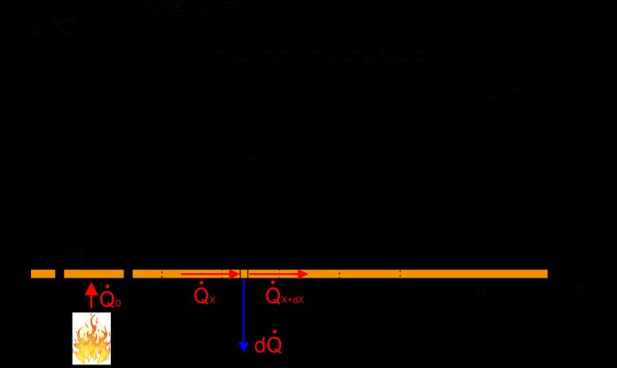
2.2 Temperature model design
 The procedure of determining a cable heating model can be divided into two stages: heating and steady state. Conductor
 temperature change rate depends on the physical conditions of the environment in the form of heat source temperature
 fields and the remaining space surrounding the cable, as well as thermal parameters of the insulating materials (thermal
 conductivity, thermal capacity).
 The manner of impact of a heat source on the cable may be determined by, e.g., fire curve or as a function of any
 temperature change waveform (e.g. step).
 Equation describing the system has the form of second order partial differential equation [1], [7]:

 2 
 ∇2 = 2 ∙ 2
 + + ( , )
 (1)
 where: k – material scale associated with thermal productivity

 The equation (1) is also called a thermal conductivity equation or a diffusion equation. The parameter φ in the
 comparison represents the temperature of cable conductors in a homogeneous environment (with constant properties in
 the set direction). It is also noted in the form:

 ∇2 = 
 (2)

 and

 2 1 
 =
 2 (3)
 the Laplace transform, we come to the operator domain. An operator form enables determining the cable conductor
 temperature T(x, t) as a response to an step function T0. For this purpose, a system with distributed parameters is replaced
 by a system with lumped parameters, described by transmittance H(x, s).
 Under the assumption that a function forcing the heat flux flow T(0, t) has the form of est, the temperature T(x, t), at any
 point with a coordinate x, is defined by a relationship:

 , = ( , ) ∙ (4)

 By substituting equation (4) to equation (3) we get:

 2 
 ∙ = ∙ ( , ) ∙ 
 2 (5)
 and
 
 − 
 , = + 
 (6)

 where A and B are constants.
 Due to the amplitude-wise finite response value, the constant A in the equation (6) must be equal to 0, otherwise the
 transmittance H(x, s) would adopt an infinite value at point x=∞, which is impossible due to the rules of physics. For this
 reason, the equation (6) takes the form:

 Proc. of SPIE Vol. 11442 114421D-3
Downloaded From: https://www.spiedigitallibrary.org/conference-proceedings-of-spie on 05 Jun 2022
Terms of Use: https://www.spiedigitallibrary.org/terms-of-use

 0 0
 − 
 , = ℒ −1 , = ℒ −1 ∙
 (7)

 Applying the inverse Laplace transform of the function included in the parentheses, we obtain an equation of a system
 with distributed parameters, in the form:

 erfc , = ∙ 0 erfc
 2 (8)

 where:
 α [W/m2 K] – thermal diffusivity coefficient, material constant
 x [m] – distance from the heat source,
 t [s] – elevated temperature impact time,
 T0 [℃] – excitation temperature (heat source).
 Notation of a cable conductor temperature model described by equation (10) contains a non-elementary supplemented
 function of the erfc error with parameters (x, t).
 A graphical representation of the T erfc(x,t) model equation solution is a temperature curve with an exponential waveform
 (Fig. 2.) [1], [12].

 Figure 2. Cooling curve theoretical waveform
 One temperature curve can be determined for each time moment.
 The impact of a fire temperature field on a cable can be divided into two stages: heating and steady state. The
 determination of the curve coefficients based on non-linear approximation of the experimental data is approximated
 more accurately, the more the temperature forcing cable heating is stabilized over time (steady state). Selecting a time
 constant τc value is of significance to the accuracy of a cable thermal model. Therefore, it is important for the results used
 to validate the model to be taken from a time moment, where the cable conductor temperature response is of a steady
 character.
 Table 1 shows the results of the heating curve time constant τop and delay time τc calculations using three different
 methods, as a response to an step excitation as a result to placing a cable in a heated-up heating chamber.

 Proc. of SPIE Vol. 11442 114421D-4
Downloaded From: https://www.spiedigitallibrary.org/conference-proceedings-of-spie on 05 Jun 2022
Terms of Use: https://www.spiedigitallibrary.org/terms-of-use

Table 1. Summary of heating time parameter calculation of studied cables
 Time
 Delay time τop
 No. Method constant τc
 [s] [s]

 1 tangent 401 62
 tangent
 2 165 62
 and point
 3 two points 127.5 84.5

 Figure 3. Cooling curve theoretical waveform

 An analytical [11] or graphical method (Fig. 3) can be used to determine a time constant. The temperature waveform
 recorded by the recorder should be used for that purpose. Due to a limited accuracy of tangent plotting, the graphical
 method is less accurate than the analytical one. It is assumed that a steady state occurs after 3÷5 time constants
 determined based on the response of a system to an excitation [5]. Cable conductor temperature response for the first
 thermocouple, counting from the cable outlet from the heating chamber, would reach 63.2% of the maximum response
 value after 1 622 seconds. Bearing in mind the results obtained through the graphical and analytical methods, we assume
 that the steady state of the heating process will occur after 1 600 seconds from the temperature excitation, with the time
 constant assumed for the calculations amounting to 400 seconds.

 3. STAND FOR TESTING CABLE HEATING

 A measuring system was constructed in order to verify the proposed model. A calculation system has to be additionally
 used in certain measuring systems, in order to obtain information about the condition of a given object. An example of
 such system in an application for testing semi-conductor materials is presented in research papers [9], [10]. The analysis
 of the electrical cable temperature measurement methods enables to select one, which would enable recording the
 temperature in the form of an electric signal, suitable for use in further calculations associated with the validation of the
 electrical cable heating mathematical model. The method utilizing thermo-elements is beneficial owing to the structural
 possibilities of thermocouple sensors, measurement accuracy and the option to utilize the obtained measurement results
 in further calculations. The test stand designed and constructed by the authors consists of: a laboratory furnace, a power
 supply system with adjusted temperature inside the heating chamber, a measuring system with temperature processing
 and recording, a supporting structure for a tested cable. Stand diagram is shown in figure 4.

 Proc. of SPIE Vol. 11442 114421D-5
Downloaded From: https://www.spiedigitallibrary.org/conference-proceedings-of-spie on 05 Jun 2022
Terms of Use: https://www.spiedigitallibrary.org/terms-of-use

Figure 4. Test stand diagram

 The furnace design enables reaching a temperature of approximately 400℃ inside the heating chamber. The hot zone
 length was 1.0m. The cable section with visible temperature changes was selected experimentally. For a cable installed
 in an open cable tray it amounted to 2.0 m. The tests involved a non-flammable (N)HXH 3x6mm2 FE180 PH90/E90
 cable, with CU ETP CW004 copper conductors, with copper content of 99.8%, which enables an assumption that the
 copper is pure in terms of material [3], [12].

 Measurements from thirteen thermocouples placed every 0.15cm along the cable, were recorded in a WRT-16M recorder
 via a RS236/USB interface and saved in a computer. The temperature recording time was 120min, which corresponds to
 the technical requirements for electrical systems powering fire-fighting equipment [14], [15], [16]. After entering into a
 computer algorithm, the measurement data were substituted into a mathematical model, and the calculation results shown
 in the form of a graph.

 4. CALCULATION RESULTS FOR THE PRESENTED MODEL

 A result of a numerical simulation of the Terfc(x, t) model is a family of exponential curves. Each curve represents a
 calculation result of conductor temperature changes along the cable within a single time moment, elapsed since the
 temperature excitation trip. The curves shown in figure 5 are derived from theoretical calculations not taking into
 account the measurement data, and are only a model simulation of the temperature waveform. The curves flatten over the
 heating time, which is a result of gradual setting of the temperature throughout the cable.

 Proc. of SPIE Vol. 11442 114421D-6
Downloaded From: https://www.spiedigitallibrary.org/conference-proceedings-of-spie on 05 Jun 2022
Terms of Use: https://www.spiedigitallibrary.org/terms-of-use

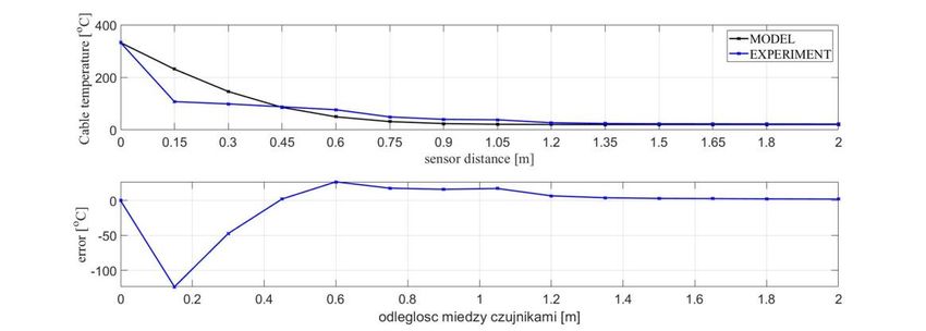
Figure 5. Model numerical simulation result.

 Inputting the measurement data into the model calculation algorithm makes the model approximate the model result to
 the experimental result of the temperature waveform. The model utilizes the classical method of least squares based on
 the Levenberg – Marquadt (algorithm L-M) algorithm to approximate the data [6], [13], [17]. The result of temperature
 calculations and approximation for any time moment equal to 2000 s from the temperature excitation trip is shown in
 figure 6a.

 Figure 6. The model approximation and calculation result: a) measurement data approximation; b) comparison
 of modelling results and experimental data.

 Using model calculation algorithm, we are able to determine the damping parameters of the temperature exponential
 curve within a studied power cable.

 ( , =2000 ) ℃ = a ∙ − (9)

 The result of the calculations for a selected time moment of 2000 seconds are coefficients a and b, which amount to: a=

 Proc. of SPIE Vol. 11442 114421D-7
Downloaded From: https://www.spiedigitallibrary.org/conference-proceedings-of-spie on 05 Jun 2022
Terms of Use: https://www.spiedigitallibrary.org/terms-of-use

328.3 [℃], b=4.637 [-], respectively.

 Parameter a is an instantaneous value of the forcing temperature. Whereas parameter b determines the slope of the
 temperature curve, which corresponds to the cable cooling rate. In the physical dimension, it represents the thermal
 diffusivity coefficient α of a conductor and electric insulation, as an entire thermal system.
 Increased coefficient α results in faster cooling of the cable. The value of coefficient α calculated by the algorithm is a
 resultant value for several insulation layers comprising the cable.
 Figure 6b shows the difference between the temperature value calculated by the model and the temperature measured
 during the experiment. The data approximation method used in the model provides satisfactory results thanks to fast
 convergences and easy implementation of the data in the model. The difference between the value calculated by the
 model relative to the experimental data is the biggest in the area of the cable closest to the heat source. This area exhibits
 the highest temperature increments, which is not beneficial for the model calculation algorithm, although, as the distance
 coordinate x increases, the algorithm generates results with an increasing accuracy.

 5. CONCLUSIONS

 The method for determining the temperature of electrical cable conductors discussed in the articles represents a new
 approach towards the determination of electrical cable heating in temperature conditions similar to a fire event. Based on
 the obtained calculation results, it is possible to determine the resistance of electrical cables, depending on the time of
 exposure to elevated ambient temperature and the distance from a heat source. This has a huge impact on the conditions
 of powering electrical equipment, especially the ones responsible for the safety of people and devices in the event of
 such dangerous phenomena as building fires. The moment of tripping of fire-fighting equipment has a large impact on
 the reliability of operation of the entire building protection system. The discussed temperature modelling method
 significantly helps the evaluation of the temperature condition of a cable system powering fire-fighting equipment. This
 method is a good tool for supporting designers of fire-fighting systems. Extending the hot zone results in a proportional
 growth of the transition zone. The scaling factors will be developed by the authors in the course of further research. The
 authors will try to expand the application range of the method onto other structural ways of laying cables than the system
 of open cable trays.

 REFERENCES

 [1] S. Zocholl, “A thermal models in power system protection”, Proceedings of the 26th Western Protective Relay
 Conferece, Spokane, WA 26-28 October 1999.
 [2] J. Wiatr and M. Orzechowski, “Instalacje elektryczne do zasilania urządzeń elektrycznych, których
 funkcjonowanie jest niezbędne w czasie pożaru”, [Electrical systems for powering electrical equipment,
 required to operate in the event of a fire], Wydanie I, Warszawa 2016.
 [3] G. Bontempi and A. Vaccaro and D. Villacci, “Power cables thermal protection by interval simulation of
 imprecise systems”, 2004 IEE Proc. Generat. Transm. Distrib.
 [4] Z. Hanzelka, “Jakość dostawy energii elektrycznej, zaburzenia wartości skutecznej napięcia”, [Electricity
 supply quality, effective voltage value disturbance]. Wydawnictwo Akademii Górniczo – Hutniczej, Kraków
 2013.
 [5] J. Kisilowski, “Podstawy technik pomiarowych”, [Basics of measurement techniques]. OBSERWACJE
 Wydawnictwo Naukowe, 2005.
 [6] S. Osowski and A. Cichocki and K. Siwek, “MATLAB w zastosowaniu do obliczeń obwodowych i
 przetwarzania sygnałów”, [MATLAB used for circuit calculations and signal processing]. Oficyna Wydawnicza
 Politechniki Warszawskiej, 2006.
 [7] T. Zaiczek and O. Enge – Rosenblatt, “Import of distributed parameter models into lumped parameter model
 libraries for the example of linearly deformable solid bodies, 3-rd International Workshop on Equation – Based
 Object – Oriented Languages and Tools”, October, 2010, Oslo, Norway.

 Proc. of SPIE Vol. 11442 114421D-8
Downloaded From: https://www.spiedigitallibrary.org/conference-proceedings-of-spie on 05 Jun 2022
Terms of Use: https://www.spiedigitallibrary.org/terms-of-use

[8] M. Suproniuk and P. Kamiński and R. Kozłowski and M. Pawłowski, “Effect of deep-level defects on transient
 photoconductivity of semi-insulating 4H-SiC”, Acta Physica Polonica A, vol. 125, pp. 1042 – 1048, 2014,
 [9] M. Suproniuk and P. Kamiński and M. Pawłowski and R. Kozłowski and M. K. Pawłowski, “An intelligent
 measurement system for characterisation of defect centres in semi-insulating materials”, Przegląd
 Elektrotechniczny, vol. 86, pp. 247 – 252, 2010,
 [10] M. Suproniuk and P. Kamiński nad M. Miczuga and M. Pawłowski and C. Longeaud and J. Kleider, “An
 intelligent measurement system for diagnosing of semi-insulating materials by photoinduced transient
 spectroscopy”, Przegląd Elektrotechniczny, vol. 86, pp. 93 – 98, 2009,
 [11] Z. Skibko, “Wpływ temperatury granicznej dopuszczalnej długotrwale i temperatury otoczenia na obciążalność
 prądową długotrwałą przewodów”, [The impact of long-term permissible limit temperature and ambient
 temperature on long-term ampacity of cables]. Wiadomości Elektrotechniczne Vol. 10/2009.
 [12] G. Angers, “Rating of Electric Power Cables in Unfavorable Thermal Environmental”, New York 2005 IEEE
 Press Series on Power Engineering.
 [13] M. Pawlowski and M. Suproniuk, “The effect of model adequacy error of the correlation method for studies of
 defect centres by photoinduced transient spectroscopy”, Przeląd Elektrotechniczny, vol. 87(10), 2011, pp. 230-
 235
 [14] Standard N SEP E-005, “Dobór przewodów elektrycznych do zasilania urządzeń przeciwpożarowych których
 funkcjonowanie jest niezbędne w czasie pożaru”, [Selection of power cables for fire-fighting equipment,
 required to operate in the event of a fire].
 [15] Catalogue of cable manufacturer TF Kable (edition IX 2009).
 [16] M. Suproniuk, P. Kamiński, P. Pawłowski, M., and Kozłowski, R., “Baza wiedzy w inteligentnym systemie
 pomiarowym do badania centrów defektowych w półprzewodnikowych materiałach półizolujących”, Przegląd
 Elektrotechniczny. 86, 247-252 (2010)
 [17] Suproniuk M., and Pawłowski M., “The effect of model adequacy error of the correlation method for studies of
 defect centres by photoinduced transient spectroscopy”, Przegląd Elektrotechniczny. 87. 230-235 (2011)

 Proc. of SPIE Vol. 11442 114421D-9
Downloaded From: https://www.spiedigitallibrary.org/conference-proceedings-of-spie on 05 Jun 2022
Terms of Use: https://www.spiedigitallibrary.org/terms-of-use