On the choice of finite element for applications in geodynamics
←
→
Page content transcription
If your browser does not render page correctly, please read the page content below
Solid Earth, 13, 229–249, 2022
https://doi.org/10.5194/se-13-229-2022
© Author(s) 2022. This work is distributed under
the Creative Commons Attribution 4.0 License.

On the choice of finite element for applications in geodynamics
Cedric Thieulot1 and Wolfgang Bangerth2
1 Department   of Earth Sciences, Utrecht University, Utrecht, the Netherlands
2 Department   of Mathematics, Department of Geosciences, Colorado State University, Fort Collins, CO, USA

Correspondence: Cedric Thieulot (c.thieulot@uu.nl)

Received: 3 June 2021 – Discussion started: 15 June 2021
Revised: 24 November 2021 – Accepted: 26 November 2021 – Published: 28 January 2022

Abstract. Geodynamical simulations over the past decades          ear systems (e.g., Donea and Huerta, 2003). This velocity–
have widely been built on quadrilateral and hexahedral fi-        pressure pair is often referred to as the Q1 × P0 Stokes el-
nite elements. For the discretization of the key Stokes equa-     ement and sometimes as the Q1 × Q0 element (Gresho and
tion describing slow, viscous flow, most codes use either the     Sani, 2000). It is used, for example, in the ConMan (King
unstable Q1 × P0 element, a stabilized version of the equal-      et al., 1990), SOPALE (Fullsack, 1995), SLIM3D (Popov
order Q1 × Q1 element, or more recently the stable Taylor–        and Sobolev, 2008), CitcomCU (Moresi and Gurnis, 1996;
Hood element with continuous (Q2 × Q1 ) or discontinuous          Zhong, 2006), CitcomS (Zhong et al., 2000; McNamara and
(Q2 × P−1 ) pressure. However, it is not clear which of these     Zhong, 2004; Zhong et al., 2008), Ellipsis (Moresi et al.,
choices is actually the best at accurately simulating “typical”   2003; O’Neill et al., 2006), UnderWorld (Moresi et al.,
geodynamic situations.                                            2003), DOUAR (Braun et al., 2008), and FANTOM (Thieu-
   Herein, we provide a systematic comparison of all of these     lot, 2011) codes and has therefore been used in hundreds of
elements for the first time. We use a series of benchmarks        publications.
that illuminate different aspects of the features we consider        The popularity of this element can be explained by its very
typical of mantle convection and geodynamical simulations.        small memory footprint and ease of implementation and use.
We will show in particular that the stabilized Q1 × Q1 el-        On the other hand, it has a rather low convergence order that
ement has great difficulty producing accurate solutions for       makes it difficult to achieve high accuracy; maybe more im-
buoyancy-driven flows – the dominant forcing for mantle           portantly, the element is known not to satisfy the so-called
convection flow – and that the Q1 × P0 element is too unsta-      Ladyzhenskaya–Babuška–Brezzi (LBB) condition condition
ble and inaccurate in practice. As a consequence, we believe      (e.g., Donea and Huerta, 2003) and is therefore unstable.
that the Q2 × Q1 and Q2 × P−1 elements provide the most           This instability noticeably manifests itself through oscilla-
robust and reliable choice for geodynamical simulations, de-      tory pressure modes (e.g., Fig. 18 of Thieulot et al., 2008
spite the greater complexity in their implementation and the      or Fig. 36 of Thieulot, 2014) and makes it not suited for
substantially higher computational cost when solving linear       large-scale three-dimensional simulations coupled to itera-
systems.                                                          tive solvers (May and Moresi, 2008). The unreliability of the
                                                                  pressure also makes this element a dubious choice for mod-
                                                                  els in which some of the parameters – e.g., the density or the
                                                                  viscosity – depend on the pressure.
1   Introduction                                                     The more modern alternative to this choice is the Taylor–
                                                                  Hood element that uses (continuous) polynomials of degree
For the past several decades, the geodynamics community’s         k for the velocity and of degree k − 1 for the pressure, where
workhorse for numerical simulations of the incompressible         k ≥ 2.1 This element is not only LBB-stable, but owing to its
Stokes equations has been the use of (continuous) piecewise
bilinear and/or trilinear velocity and piecewise constant (dis-       1 Strictly speaking, Taylor and Hood (1973) only introduced the
continuous) pressure finite elements, often in combination        Q2 × Q1 element on quadrilaterals. However, finite-element practi-
with the penalty method for the solution of the resulting lin-    tioners use the term “Taylor–Hood” for both the 2D and 3D cases,

Published by Copernicus Publications on behalf of the European Geosciences Union.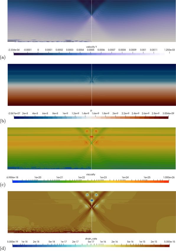
230                                                                        C. Thieulot and W. Bangerth: Q1 × Q1 -stab in geodynamics

higher polynomial degree is also convergent of higher order.                  lowing for the numerical solution of whole Earth models at
It is therefore widely used in commercial flow solvers and                    high resolutions (Stadler et al., 2010; Alisic et al., 2012).
is also the default element for the A SPECT code in geody-                    Another example of the use of this method is the work of
namics (Kronbichler et al., 2012; Heister et al., 2017). This                 Leng and Zhong (2011), also using AMR, to study thermo-
element is obviously more difficult to implement, and build-                  chemical mantle convection. Both the ELEFANT code with
ing efficient solvers and preconditioners is also more com-                   an application to the 3D thermal state of curved subduction
plicated (Kronbichler et al., 2012; Clevenger et al., 2020).                  zones (Plunder et al., 2018) and the GALE code (Moresi
However, these drawbacks can be mitigated by building on                      et al., 2012), with application to the 3D shapes of metamor-
one of the widely available finite-element libraries that have                phic core complexes (Le Pourhiet et al., 2012) or oceanic
appeared over the past 20 years; for example, A SPECT in-                     plateau subduction (Arrial and Billen, 2013), use the stabi-
herits all of its finite-element functionality from the deal.II               lized Q1 × Q1 method. Finally the ADELI code was cou-
library (see Bangerth et al., 2007; Arndt et al., 2020). We                   pled to a stabilized Q1 × Q1 flow solver in the context of
will note that one can also use a number of variations of the                 lithosphere–asthenosphere interaction studies (Cerpa et al.,
underlying idea of the Taylor–Hood element, for example on                    2014, 2015, 2018).
quadrilaterals and hexahedra by using Qk ×P−(k−1) (see, for                      The availability of all of these options leads us to the main
instance, May et al., 2015, Lechmann et al., 2011, and Thiel-                 question of this paper: which element should one use in geo-
mann and Kaus, 2012) in which the pressure is discontinuous                   dynamics computations based on the Stokes equations? Or,
and of (total) polynomial degree k − 1, but missing the part                  in the absence of clear-cut conclusions, which ones should
of the finite-element space on every cell that distinguishes the              not be used? On the face of it, this seems like a simple
space Qk on quadrilaterals and hexahedra from the space Pk                    question: the consensus in the computational science com-
that is typically used on triangles and tetrahedra.2 Another                  munity is that using moderately high-degree elements (say,
variation is to enrich the pressure space by a constant shape                 k = 3 or k = 4) yields the best accuracy for a given compu-
function on each cell (see, for example, Boffi et al., 2011,                  tational effort (measured in CPU cycles) unless one wants
and the references therein). All of these alternatives are sta-               to change the solver technology to use matrix-free methods
ble for k ≥ 2, and in keeping with common usage of the term,                  whereby even higher polynomial degrees become more ef-
we will also refer to all of these variations as Taylor–Hood                  ficient. This conclusion is based on the higher convergence
or Taylor–Hood-like elements even though they are strictly                    order of higher-degree methods but balanced by the rapidly
speaking not what Taylor and Hood proposed in Taylor and                      growing cost of matrix assembly and linear solver effort for
Hood (1973).                                                                  higher-degree methods. On the other hand, the recommen-
   A third option is the use of Q1 × Q1 elements with both                    dation to use higher-degree methods is predicated on the as-
velocity and pressure using bilinear or trilinear shape func-                 sumption that the solution is smooth enough – say, the ve-
tions. This combination of elements is not LBB-stable by                      locity is in the Sobolev space H k+1 of functions that have,
default, but numerous stabilization techniques – typically                    loosely speaking, at least k + 1 derivatives – that one can
adding a pressure-dependent term to the mass conservation                     actually achieve a convergence rate of O(hk ) in the energy
equation – have been proposed in the literature (see, e.g.,                   norm and O(hk+1 ) in the L2 norm, where h is the mesh size.
Norburn and Silvester, 2001; Elman et al., 2014; Gresho                       This assumption generally requires that all coefficients, such
et al., 1995). Herein, we will discuss in particular the vari-                as density and viscosity, are sufficiently smooth on length
ation by Dohrmann and Bochev (2004) that is simple to im-                     scales resolvable by the mesh. This may not be the case in
plement and does not involve any tunable parameter. This ap-                  realistic geodynamics problems given that density and vis-
proach is used in the Rhea code (Burstedde et al., 2009, 2013)                cosity often depend discontinuously on the solution variables
in conjunction with adaptive mesh refinement (AMR), al-                       (velocity or strain rate, pressure, temperature, and composi-
                                                                              tional variables); indeed, in many models, the viscosity may
for the case of both simplex and quadrilateral–hexahedral meshes,             vary by orders of magnitude on short length scales.
and for all cases with k ≥ 2. See also John (2016, p. 98).                       Such considerations put into question whether higher-
    2 The discontinuous space P
                                  −(k−1) for the pressure can be inter-       order methods are really worth the effort for actual geo-
preted in two incompatible ways: first, one can map the correspond-           dynamics simulations. Given these divergent theoretical
ing space from the reference cell to each of the cells of the mesh,           thoughts, the only way to resolve the question is by way of
as one also does for the velocity; or, one can define shape functions         numerical comparisons. We have consequently extended A S -
directly in the global coordinate system, without mapping from the
                                                                              PECT so that it can use all of the element combinations above,
reference cell. The two agree on cells that are parallelograms but not
on more general meshes. Since our experiments are all on meshes
                                                                              and we will use these implementations in the comparisons in
where all cells are rectangles, the distinction does not matter for the       this paper.
current paper, but we point out that the error estimates (Eq. 4) stated          Goals of this paper. Having outlined the conflict between
in Sect. 3.1 only hold for the latter definition. See Boffi and Gastaldi      the expected superiority of higher-degree elements for the
(2002), Matthies and Tobiska (2002), and John (2016, Sect. 3.6.4)             Stokes equation on the one hand and the expected lack of
for more information.

Solid Earth, 13, 229–249, 2022                                                                     https://doi.org/10.5194/se-13-229-2022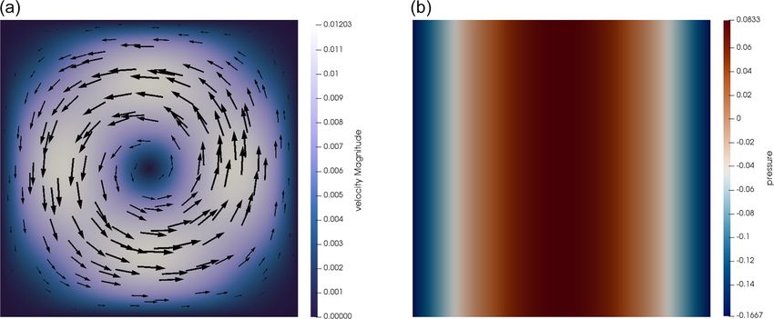
C. Thieulot and W. Bangerth: Q1 × Q1 -stab in geodynamics                                                                        231

smoothness of solutions in realistic geodynamic cases, our               driven by buoyancy variations (May et al., 2015).
goals in the paper are as follows.                                       In geophysical flow models this yields unphysical
                                                                         pressure artifacts for cases where both the free sur-
 1. Quantitatively compare the solution accuracy of the var-             face of the Earth and mantle flow are considered,
    ious options (Q1 × P0 , Qk × Qk−1 , Qk × P−(k−1) and                 because the driving density contrast between cold
    stabilized Q1 × Q1 ) using a variety of analytical bench-            sinking plates and the warmer surrounding Earth’s
    marks for which the exact solution is known. As we                   mantle is much smaller than the density difference
    will see below, there is little point working with k > 2             between rocks and air (Kaus et al., 2010; Popov
    in geodynamics applications, and so the only cases we                and Sobolev, 2008; Mishin, 2011). In our experi-
    consider for Taylor–Hood-like elements are Q2 × Q1                   ence, this results in artificial “compaction” of the
    and Q2 × P−1 .                                                       Earth’s mantle if Q1 × Q1 /stab element is used,
                                                                         which makes them unsuitable for these purposes.
 2. Extend these numerical comparisons to cases in which it
    is known that the stabilized Q1 ×Q1 demonstrates prob-           Indeed, our numerical experiments will encounter a simi-
    lematic behavior that may make it unusable in many            lar issue; see Sect. 6.
    practical situations. In particular, we will consider the        We are not aware of any other significant publications in
    case of buoyancy-driven flows.                                the geodynamics literature that specifically discuss the rel-
                                                                  ative trade-offs between the elements we consider herein,
 3. Conclude our considerations by comparing the available        specifically between the Q1 ×P0 and Taylor–Hood elements,
    options using a realistic geodynamical application. This      and consequently believe that our discussions here are useful
    will allow us to draw conclusions as to what element          for the community.
    one might want to recommend for geodynamics appli-
    cations.
                                                                  2     The governing equations
   While we have approached this study with an open mind
and without a strong prior idea of which element might be         For the purpose of this paper, we are concerned with the ac-
the best, let us end this Introduction by noting that mem-        curate numerical solution of the incompressible Stokes equa-
bers of the crustal dynamics and mantle convection commu-         tions:
nities have occasionally expressed a dislike of the stabilized
Q1 ×Q1 element for its inability to deal with large lithostatic   −∇ · [2ηε(u)] + ∇p = ρg                     in ,              (1)
pressures and free surfaces absent special modifications of                       −∇ · u = 0                  in ,              (2)
the formulation. For example, Arrial and Billen (2013) com-
ment on the need to modify the physical description of the        where η is the viscosity, ρ the density, g the gravity vec-
problem due to the stabilization (with references replaced by     tor, ε(·) denotes the symmetric gradient operator defined by
ones listed at the end of this paper).                            ε(u) = 21 (∇u+∇uT ), and  ⊂ Rd , d = 2 or 3 is the domain
                                                                  of interest. Both the viscosity η and the density ρ will, in
     All the models were run with the open source code            general, be spatially variable; in applications, this is often
     Gale. [. . . ] Gale uses Q1 –Q1 elements to describe         through nonlinear dependencies on the strain rate ε(u) or the
     the pressure and the velocity. However, this formu-          pressure, but the exact reasons for the spatial variability are
     lation is unstable and a slight compressible term            not of importance to us here: what matters is that these coef-
     is added in the divergence equation to stabilize it          ficients may vary strongly and on short length scales.
     (Dohrmann and Bochev, 2004). Ideally, this term                 In applications, the equations above will be augmented by
     should be applied on the dynamic pressure and not            appropriate boundary conditions and will be coupled to addi-
     on the full pressure. To fix this, a hydrostatic term        tional and often time-dependent equations, such as ones that
     corresponding to the reference density and temper-           describe the evolution of the temperature field or of the com-
     ature profile, is subtracted from the full pressure          position of rocks (see, for example, Schubert et al., 2001;
     and the body force vector.                                   Turcotte and Schubert, 2012). This coupling is also not of
                                                                  interest to us here.
  Few other negative comments concerning the Q1 × Q1 el-
ement appear on record in the published literature, although
one can find the following quote in Lehmann et al. (2015).        3     Discretization using finite-element methods
     We do not consider the Q1 × Q1 /stab element                 3.1    Formulation and basic error estimates
     (Dohrmann and Bochev, 2004; Bochev et al.,
     2006; Burstedde et al., 2009), as stabilization of           For the comparisons we intend to make in this paper,
     this element is achieved by introducing an artificial        Eqs. (1)–(2) are discretized using the finite-element method.
     compressibility that dominates for flows mainly              A straightforward application of the Galerkin method yields

https://doi.org/10.5194/se-13-229-2022                                                           Solid Earth, 13, 229–249, 2022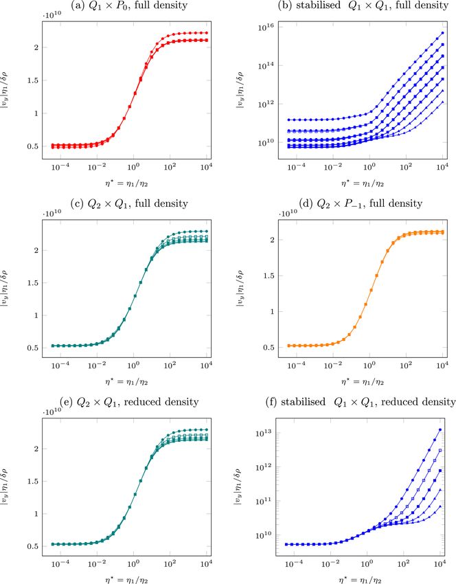
232                                                                     C. Thieulot and W. Bangerth: Q1 × Q1 -stab in geodynamics

the following finite-dimensional variational problem: find                 Here, I is the identity operator and π0 is the projection onto
uh ∈ Uh , ph ∈ Ph so that                                                  piecewise constant functions – i.e., π0 f is the function that
                                                                           on each cell is equal to the mean value of f on that cell. For
(ε(v h ), 2ηε(uh )) − (∇ · v h , ph ) = (v h , ρg),                        this element, the rates one might hope for are as follows (see
                    −(qh , ∇ · uh ) = 0,                         (3)       again Dohrmann and Bochev, 2004):

R all test functions v h ∈ Uh , qh ∈ Ph . Here, (a, b) =
for                                                                        k∇(u − uh )kL2 = O(h),
   a(x)b(x) dx. For simplicity, we have omitted terms in-                       ku − uh kL2 = O(h2 ),
troduced through the treatment of boundary conditions. The
finite-dimensional, piecewise polynomial spaces Uh and Ph                        kp − ph kL2 = O(h).                                          (7)
can be chosen in a variety of ways, as discussed in the In-
troduction. In particular, if they are chosen as Uh = Qk and               Dohrmann and Bochev (2004) report that for some test cases,
Ph = Qk−1 – i.e., the Taylor–Hood element – then the dis-                  one might in fact obtain kp − ph kL2 = O(ht ) with t ≈ 1.5,
crete problem is known to satisfy the LBB condition and the                though it is not clear whether this rate can be obtained for all
solution is stable (Elman et al., 2014). Here, Qs is the space             possible applications. We also observe this improved rate in
of continuous functions that are obtained on each cell K of                one of our benchmarks in Sect. 5.
a mesh T by mapping polynomials of degree at most s in                        We end this section by noting that in many of the setups
each variable from the reference cell [0, 1]d . Likewise, the              we use in Sect. 5, the boundary conditions we impose lead
problem is stable if one chooses Uh = Qk and Ph = P−(k−1) ,                to a problem in which the pressure is only determined up
where now P−s is the space of discontinuous functions ob-                  to an additive constant. The same is then true for the lin-
tained by mapping polynomials of total degree at most s from               ear system one has to solve after discretization. As a conse-
the reference cell. In both of these cases, we expect from                 quence, we can only meaningfully compute quantities such
fundamental theorems of the finite-element method (see, for                as kp − ph kL2 if both the exact and the numerical solution
example, Elman et al., 2014) that the convergence rates are                are normalized; a typical normalization is to ensure that their
optimal, i.e., that the errors satisfy the relationships                   mean values are zero. A SPECT enforces this normalization
                                                                           after solving the linear system.
k∇(u − uh )kL2 = O(hk ),
                                                                           3.2    A closer look at the error estimates
      ku − uh kL2 = O(hk+1 ),
    kp − ph kL2 = O(hk ),                                        (4)       A comparison of Eq. (4) with Eqs. (5) and (7) would suggest
                                                                           that the Taylor–Hood element can obtain substantially bet-
where h is the maximal diameter over all cells in the mesh T.              ter rates of convergence if one only chooses the polynomial
   On the other hand, if one chooses Uh = Q1 and Ph = P0 ,                 degree k large enough.
i.e., the unstable Q1 × P0 element with piecewise linear con-                 However, this is an incomplete understanding because the
tinuous velocities and piecewise constant discontinuous pres-              O(hm ) notation hides the fact that the constants in this be-
sure, then the best convergence rates one can hope for would               havior depend on the solution. More specifically, a complete
satisfy the following relationships based solely on interpola-             description of the error behavior would replace Eq. (4) by the
tion error estimates:                                                      following statement: there are constants C1 , C2 , C3 < ∞ so
                                                                           that
k∇(u − uh )kL2 = O(h),
      ku − uh kL2 = O(h2 ),                                                k∇(u − uh )kL2 ≤ C1 hk k∇ k+1 ukL2 ,
    kp − ph kL2 = O(h).                                          (5)             ku − uh kL2 ≤ C2 hk+1 k∇ k+1 ukL2 ,

In practice, if the numerical solution shows pressure oscil-                     kp − ph kL2 ≤ C3 hk k∇ k pkL2 .                              (8)
lations (see for instance Sani et al., 1981a, b), one will not
                                                                           The validity of these statements clearly depends on the so-
even observe the rates shown above but might in fact obtain a
                                                                           lution being regular enough so that ∇ k+1 u and ∇ k p actu-
worse pressure convergence rate, for example kp − ph kL2 =
                                                                           ally exist and are square-integrable – in other words, that u ∈
O(h1/2 ).
                                                                           H k+1 and p ∈ H k , where H k represents the usual Sobolev
   Finally, if one uses Uh = Q1 and Ph = Q1 , then this unsta-
                                                                           function spaces. 3 On the other hand, all that is guaranteed by
ble element combination can be made stable if one replaces
the discrete formulation (3) by the following stabilized ver-                 3 For a concise definition of the Lebesgue space L and the
                                                                                                                                   2
sion due to Dohrmann and Bochev (2004):                                    Sobolev spaces of functions H k , see Elman et al. (2014). Loosely
                                                                           speaking, L2 is the set of all Rfunctions f for which the integral
              (ε(v h ), 2ηε(uh )) − (∇ · v h , ph ) = (v h , ρg),          of the square over the domain,  |f (x)|2 dx, is finite. We say that
                                                                           such functions are “square-integrable”. H k is the set of all functions

                                 1
(qh , ∇ · uh ) − (I − π0 )qh , (I − π0 )ph = 0.                   (6)      whose kth (weak) derivatives are square-integrable.
                                 η

Solid Earth, 13, 229–249, 2022                                                                    https://doi.org/10.5194/se-13-229-2022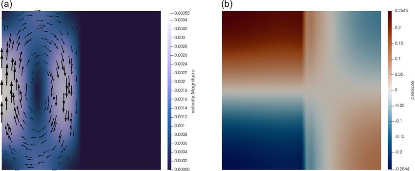
C. Thieulot and W. Bangerth: Q1 × Q1 -stab in geodynamics                                                                      233

the existence theory for partial differential equations is that    convergence rates between the minimal theoretically guar-
u ∈ H 1 and p ∈ L2 = H 0 ; any further smoothness should           anteed and the optimal ones – for some elements even if the
only be expected if, for example, the domain  is convex           solution lacks regularity. Actually observing the minimal the-
and if viscosity η and right-hand side ρg are also smooth.         oretically guaranteed convergence rate for solutions lacking
Indeed, this is the case for many artificial benchmarks for        regularity often requires choosing randomly arranged meshes
which these functions are chosen a priori; on the other hand,      – a case we will not consider herein.
in “realistic” geodynamics applications, one might expect η
and ρ to be discontinuous at phase boundaries and poten-
tially vary widely. In such cases, one needs to accept that the    4   Comments about the use of the Q1 × Q1 element in
solutions only satisfy u ∈ H q and p ∈ H q−1 with q ≥ 1 but            geodynamics computations
possibly q < k + 1. Numerical analysis predicts that in such
cases, the best-case rates in Eq. (8) will be replaced by the      Before delving into the details of numerical experiments,
following:                                                         let us consider one other theoretical aspect. An interesting
                                                                   complication of geodynamics simulations compared to many
k∇(u − uh )kL2 ≤ C1 hmin{q−1,k} k∇ min{q,k+1} ukL2 ,               other applications of the Stokes equations is that the hydro-
    ku − uh kL2 ≤ C2 hmin{q,k+1} k∇ min{q,k+1} ukL2 ,              static component of the pressure is often vastly larger than
                                                                   the dynamic pressure, even though only the dynamic com-
   kp − ph kL2 ≤ C3 hmin{q−1,k} k∇ min{q−1,k} pkL2 .        (9)    ponent is responsible for driving the flow. As we will dis-
   Similar considerations apply for the Q1 × P0 and the sta-       cuss in the following, this has no importance when using the
bilized Q1 × Q1 combinations; a closer examination yields          Q1 × P0 or the Taylor–Hood elements, but it turns out to be
the following rates that would replace Eqs. (5) and (7):           rather inconvenient when using a stabilized formulation that
                                                                   contains an artificial compressibility term. This issue is also
k∇(u − uh )kL2 ≤ C1 hmin{q−1,1} k∇ min{q,2} ukL2 ,                 mentioned in the quote from Arrial and Billen (2013) repro-
    ku − uh kL2 ≤ C2 hmin{q,2} k∇ min{q,2} ukL2 ,                  duced in the Introduction and in May et al. (2015).
                                                                      To illustrate the issue, consider the force balance equation
   kp − ph kL2 ≤ C3 hmin{q−1,1} k∇ min{q−1,1} pkL2 .       (10)    (Eq. 1). We can split the pressure into hydrostatic and dy-
   In other words, we will only benefit from the added ex-         namic components, p = ps +pd , where we define the hydro-
pense of the Taylor–Hood element with k ≥ 2 if the solution        static pressure via the relationship
is sufficiently smooth, namely if at least q > k ≥ 2. The ques-    ∂
tion of whether q > 2 indeed for a given situation is one of          ps = ρref (z)gz (z),                                    (11)
                                                                   ∂z
partial differential equation (PDE) theory and difficult to an-
swer in general without using particular knowledge of η, ρg,       coupled with the normalization that ps = 0 at the top of
and . On the other hand, one can observe convergence rates        the domain. In defining ps this way, we have made the as-
experimentally for a number of cases of interest, so in some       sumption that the vertical component gz of the gravity vector
sense, it would be legitimate to ask the following question:       dominates its other components. Furthermore, we have intro-
what is the regularity index q of typical solutions in geody-      duced a reference density ρref that somehow reflects a depth-
namics applications? At the same time, this requires careful       dependent profile. As we will discuss below, there is really
convergence studies on problems that are already typically         no unique or accepted way to define this profile, though one
quite challenging to solve on any reasonable mesh, let alone       should generally think of it as capturing the bulk of the three-
several further refined ones. As a consequence, we cannot          dimensional variation in the density via a one-dimensional
answer this question in the generality stated above. Instead,      function.
we will approach it below by considering a number of bench-           By splitting the pressure in this way, Eq. (1) can then be
marks that illustrate typical features of geodynamic settings      rewritten as follows:
in an abstracted way (in Sect. 5), followed by a model ap-
plication (in Sect. 6). In particular, the examples in Sect. 5.2   −∇ · [2η(u)] + ∇pd = ρg − ρref gz ez      in .
and 5.3 will illustrate cases in which the exact solution is not
smooth enough to achieve the optimal convergence rate.             Since this is the only equation in which the pressure ap-
   We end this section by noting that all of the estimates         pears, it is obvious that the velocity field so computed is
shown above guarantee that the error on the left of an in-         the same whether or not one uses the original formulation
equality decreases at least at the rate shown on the right side,   solving for u and p or the one solving for u and pd . More
but they do not state that on a given sequence of meshes,          concisely, the observation shows that the velocity field so
the rate might not in fact be better. Indeed, this often hap-      computed does not depend on how one chooses the refer-
pens: for example, if one aligns meshes with a discontinu-         ence density ρref . The original formulation is recovered by
ity in coefficients (as we do for the SolCx benchmark dis-         using the simplest choice, ρref = 0. As a consequence, many
cussed in Sect. 5.2), one often observes optimal rates – or        geodynamics codes use formulations that only compute the

https://doi.org/10.5194/se-13-229-2022                                                          Solid Earth, 13, 229–249, 2022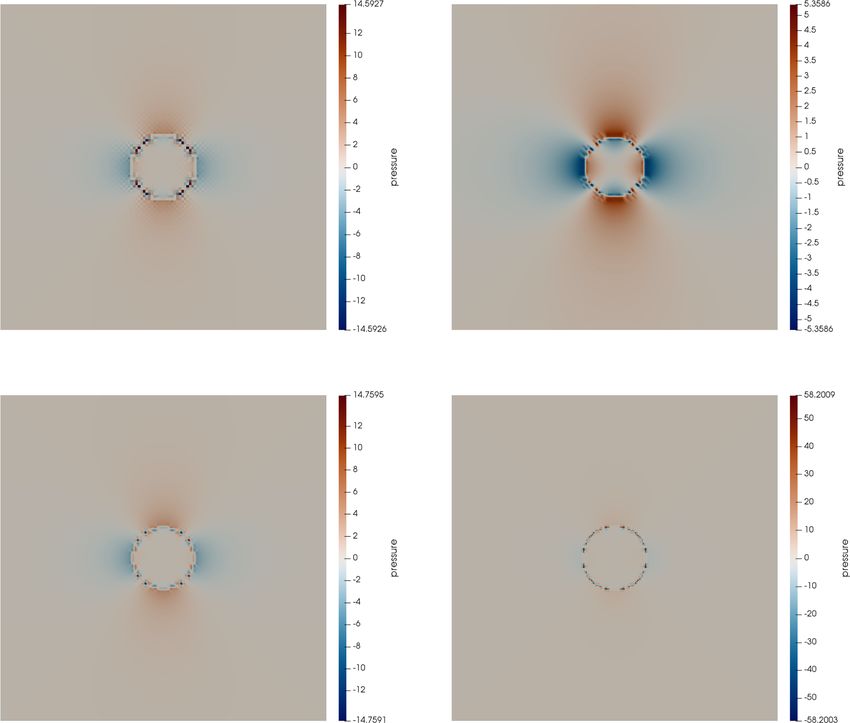
234                                                                     C. Thieulot and W. Bangerth: Q1 × Q1 -stab in geodynamics

dynamic pressure pd using a reference density ρref (z). Im-                driven by buoyancy effects but by inflow and outflow bound-
portantly, however, there is no canonical way for this defini-             ary conditions (e.g., Turek, 1999; Zienkiewicz and Taylor,
tion: one might choose a constant reference density, a depth-              2002). Indeed, in those conditions both the density and the
dependent adiabatic profile, or one computed at each time                  gravity vector are generally considered spatially constant,
step by laterally averaging the current three-dimensional den-             and the choice of reference density and hydrostatic pressure
sity field ρ(x, y, z, t); each of these options – and likely more          is then obvious and unambiguous. In these cases, computa-
– have been used in numerical simulations one can find in                  tions are always performed with only the dynamic pressure
the literature. In any case, pressure-dependent coefficients               because the hydrostatic pressure does not enter the prob-
such as the density or viscosity are then evaluated by using               lem at all except in the rare cases of fluids with pressure-
ps + pd , where pd is computed as part of the solution of the              dependent viscosities.
Stokes problem and ps is the hydrostatic pressure defined                     Second, while we have here considered the stabilization
by Eq. (11) using the particular choice of reference density               first introduced in Dohrmann and Bochev (2004), earlier sta-
used by a code. On the other hand, the A SPECT code no-                    bilized formulations used a pressure Laplacian in place of the
tably always computes the full pressure instead of splitting it            operator 5 above. (See, for example, Brezzi and Pitkäranta,
in hydrostatic and dynamic components (see the discussion                  1984, or the variation in Silvester and Kechkar, 1990, as well
in Kronbichler et al., 2012) corresponding to the particular               as the analysis in Bochev et al., 2006.) That is, instead of
choice ρref = 0.                                                           Eq. (12) they used a formulation of the form
   The problem with the stabilized Q1 × Q1 formulation –
different from the use of the other element choices – is that              −∇ · u − ch2 1p = 0,                                       (13)
the velocity field computed from the Stokes solution is not
                                                                           where c is a tuning parameter that also incorporates the vis-
independent of the choice of the reference density. This is
                                                                           cosity. If one uses this formulation for cases in which the ref-
because the mass conservation equation is modified by the
                                                                           erence density is chosen as a function that is constant in depth
stabilization term and – in the simple case of a constant vis-
                                                                           – as was often done in earlier mantle convection codes con-
cosity – reads
                                                                           sidering the Boussinesq approximation – and if one computes
        1                                                                  in a Cartesian box with a constant gravity vector g = gez ,
−∇ · u − 5pd = 0.                                               (12)       then ps is a linear function, and consequently 1ps = 0. In
        η
                                                                           other words, 1p = 1(p−ps ) = 1pd , which implies that the
Here, 5 = (I − π0 ) is the operator that corresponds to the                computed velocity field again did not depend on the exact
stabilization term in Eq. (6). 4                                           choice of ρref as long as it was chosen constant. This property
   The point of these considerations is that different choices             does not hold for the formulation of Dohrmann and Bochev
of ρref (including the choice ρref = 0 that leads to the orig-             because 5p 6 = 5(p − ps ) = 5pd for linear pressures ps be-
inal formulation) do have an effect here because they lead                 cause 5ps 6 = 0: 5 subtracts from ps the average value on
to different pd = p − ps for which 5pd is different: that                  each cell, leaving a piecewise linear discontinuous function.
is, the amount of artificial compressibility depends on the                   Of course, whether one uses the Dohrmann–Bochev for-
splitting of the pressure into static and dynamic pressures.               mulation (Eq. 12) or the addition of a pressure Laplace as in
In other words, the discretization errors ku − uh kL2 and                  Eq. (13), the formulation is consistent. That is, as the mesh
k∇(u − uh )kL2 discussed in the previous section will in gen-              size h goes to zero, the added stabilization term also goes to
eral depend on the choice of the reference density profile, and            zero. In the limit, the numerical solution therefore satisfies
the latter will need to be carefully defined in order to lead to           the original mass conservation equation. In other words, the
acceptable error levels. As we will show in the benchmarking               limit is independent of the choice of ρref , even though the
section, the specific choice of ρref in fact has a rather large ef-        solutions on a finite mesh are not.
fect. This is in line with the previously quoted comments in
Arrial and Billen (2013).
                                                                           5   Numerical results for artificial benchmarks
   Let us end this section by commenting on two aspects of
why this issue may not be as relevant in other contexts in                 In this section, let us present computational results for three
which stabilized formulations have been used. First, in many               analytical problems and a buoyancy-driven flow community
important applications of the Stokes equations, the flow is not            benchmark. While the first of these (Sect. 5.1) is simply used
   4 To                                                                    to establish the best convergence rates one can hope for in
             arrive at this form for the operator, one needs             the case of smooth solutions, the remaining test cases were
to rewrite Eq. (6) using               (I − π0 )qh , η1 (I − π0 )ph =
                                                                         chosen because they illustrate aspects of what we think “typ-
  qh , η1 (I − π0 )∗ (I − π0 )ph , where the asterisk denotes the          ical” solutions of geodynamic applications look like in an
adjoint operator. One then shows (I − π0 )∗ = (I − π0 ) and finally        abstracted, controlled way. In particular, the “SolCx” bench-
that 5 = (I − π0 )2 = I − π0 , which follows by recalling that             mark in Sect. 5.2 demonstrates features of solutions in which
projection operators are idempotent.                                       the mesh can be aligned with sharp features in the viscos-

Solid Earth, 13, 229–249, 2022                                                                  https://doi.org/10.5194/se-13-229-2022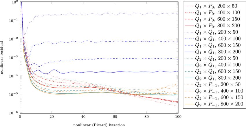
C. Thieulot and W. Bangerth: Q1 × Q1 -stab in geodynamics 235
ity, and the “SolVi” benchmark in Sect. 5.3 does so in the Finally, we also investigate the cost associated with solv-
more common case in which the mesh cannot be aligned. Fi- ing this problem using the various elements. Fig. 3 shows
nally, the “sinking block” case in Sect. 5.4 shows a buoyancy- the number of outer FGMRES iterations (Kronbichler et al.,
driven situation in which all of the discussions of the previ- 2012) iterations of the Stokes solver as a function of the mesh
ous section on the choice of a reference density will come size.5 This number is nearly constant with increasing reso-
into play. All of these cases are simple enough that we know lution for the stable or stabilized elements, while it becomes
(quantitative or qualitative features of) the solution to suffi- exceedingly large for the unstable Q1 ×P0 element, reflecting
cient accuracy to investigate convergence rigorously. the fact that lack of LBB stability corresponds to the smallest
While these benchmarks provide us with insight that al- eigenvalue of the system matrix tending to zero – and thereby
lows us to conjecture which elements may or may not work in driving the condition number to infinity. Indeed, our linear
practical application, they still are just abstract benchmarks. solver does not converge in the 1000 iterations we chose as a
As a consequence, we will consider an actual geodynamic limit for the smallest mesh sizes.
application in Sect. 6.
All models are run with the A SPECT code. We have lim- 5.2 The SolCx benchmark
ited ourselves to two-dimensional cases as we do not expect
that three-dimensional models would shed any more light on The SolCx benchmark is a common benchmark found in
the conclusions reached. Although A SPECT is built for adap- many geodynamical papers (e.g., Zhong, 1996; Duretz et al.,
tive mesh refinement (AMR), we have chosen not to use this 2011; Kronbichler et al., 2012; Thielmann et al., 2014). It
feature in order to reflect the fact that the majority of existing uses a discontinuous viscosity profile with a large jump in
codes use structured meshes. the viscosity value along the middle of the domain, result-
ing in a discontinuous pressure field. The domain is a unit
5.1 The Donea and Huerta benchmark square, boundary conditions are free-slip on all edges, and
the gravity vector points downwards with |g| = 1. The den-
Let us start our numerical experiments with the simple 2D sity for SolCx is given by ρ(x, y) = sin(πy) cos(π x) and the
benchmark presented in Donea and Huerta (2003). The ex- viscosity field is such that
act definition involves lengthy formulas not worth repeat-
1, if 0 ≤ x ≤ 0.5
ing here, but in short it consists of the following ingredients: η(x, y) =
106 if 0.5 < x ≤ 1.
(i) the domain is a unit square, (ii) the viscosity and density
are set to 1, and (iii) velocity and pressure fields are cho- We show the velocity and pressure fields in Fig. 4. The
sen to correspond to smooth polynomials describing circular discontinuous jump of the viscosity field by a factor of 106
flow with no-slip boundary conditions. We then choose an results in separate convective cells on the left and right sides
(unphysical) gravity vector field that produces these velocity of the domain, though with vastly different strengths. The
and pressure fields. This setup produces the smooth solution pressure also reflects this disjoint behavior.
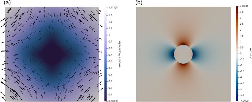
shown in Fig. 1 for which we would expect that the higher- As in the Donea and Huerta benchmark, we compute the
order Taylor–Hood element is highly accurate. velocity and pressure error convergence for all four elements.
We verify this in Fig. 2 for the four element choices of Those are shown in Fig. 5. As documented in Kronbich-
interest in this work: Q1 × P0 , stabilized Q1 × Q1 , Q2 × Q1 , ler et al. (2012), the second-order element with discontinu-
and Q2 × P−1 . Looking at the velocity error, we recover a ous pressure Q2 × P−1 performs better (pressure error con-
cubic convergence rate (q = 3) for the Q2 ×Q1 and Q2 ×P−1 vergence is O(h2 )) than its continuous pressure counterpart
elements and a quadratic convergence rate (q = 2) for those Q2 × Q1 (convergence is only O(h1/2 ), but the better con-
choices using the Q1 elements for the velocity. The pressure vergence order with the discontinuous pressure can only be
error is of linear rate for the Q1 ×P0 element and of quadratic obtained if the discontinuity in the viscosity is aligned with
rate for the Q2 ×Q1 and Q2 ×P−1 elements. All of these are cell boundaries – which is the case here. Also of interest here
as expected. For the stabilized Q1 ×Q1 , we obtain the better- is the fact that the Q1 × P0 outperforms the Q1 × Q1 ele-
than-expected rate of 1.5 already mentioned in Dohrmann ment for both velocity and pressure. All of these observa-
and Bochev (2004); see also Sect. 3. tions are readily explained by the fact that a discontinuous
Figure 3 shows the root mean square velocity as a function pressure can only be approximated well when using discon-
of the mesh size as obtained with the four elements in ques- tinuous pressure elements with cell interfaces aligned with
tion. Again, the second-order elements are more accurate. the discontinuity in the viscosity.
These results are not surprising: the solution is smooth, Figure 6 shows the number of outer FGMRES iterations of
and consequently one would expect to obtain optimal order the Stokes solver as a function of the mesh size. We find this
convergence in all cases. One can carry out similar experi- 5 The concrete number of iterations of course depends on the
ments for the SolKz benchmark (Zhong, 1996), which also preconditioner used – here the one described in Kronbichler et al.
has a smooth solution; we have obtained identical error con- (2012). The important point of the figure, however, is how the num-
vergence rates. ber of iterations changes (or does not) with the mesh size h.
https://doi.org/10.5194/se-13-229-2022 Solid Earth, 13, 229–249, 2022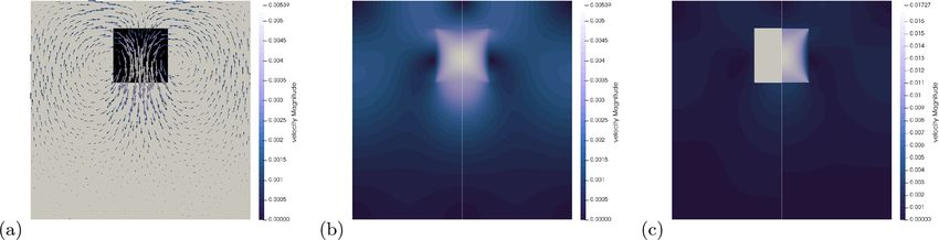
236                                                                  C. Thieulot and W. Bangerth: Q1 × Q1 -stab in geodynamics

Figure 1. Donea and Huerta benchmark. Velocity (a) and pressure (b) fields obtained on a 32 × 32 mesh with Q2 × Q1 elements.

Figure 2. Donea and Huerta benchmark. Error convergence as a function of the mesh size h. (a) Velocity error ||u − uh ||L2 . (b) Pressure
error ||p − ph ||L2 . The two leftmost points are missing for Q1 × P0 since the solver failed to converge; the data points for Q2 × Q1 and
Q2 × P−1 are on top of each other.

time that this number is nearly constant with increasing res-           cult to represent accurately. Using the regular meshes used
olution for all four elements. Unsurprisingly the Q1 × P0 el-           by a majority of codes, the discontinuity in the viscosity and
ement requires more iterations than all the others but by less          pressure then never aligns with cell boundaries. Even though
than a factor of 2. The quadratic elements require the same             A SPECT can use arbitrary unstructured meshes (and can also
number of iterations, while the stabilized Q1 × Q1 requires             use curved cell edges), we will honor the setup of this bench-
only half their number: this is surprising, but the conclusions         mark by only considering regular meshes.
from the previous paragraph remain about it being the least                Schmid and Podlachikov (2003) derived a simple analyti-
accurate of all four elements here.                                     cal solution for the pressure and velocity fields for such a cir-
                                                                        cular inclusion under pure shear, and this benchmark is show-
5.3   The SolVi (circular inclusion) benchmark                          cased in many publications (Deubelbeiss and Kaus, 2008;
                                                                        Suckale et al., 2010; Duretz et al., 2011; Kronbichler et al.,
The SolCx benchmark in the previous section allows for                  2012; Gerya et al., 2013; Thielmann et al., 2014). The veloc-
aligning mesh interfaces with the discontinuity in the vis-             ity and pressure fields are shown in Fig. 7.
cosity. This is an artificial situation that will, in general, not         A characteristic of the analytic solution is that the pres-
happen in actual large-scale geodynamics applications for               sure is zero inside the inclusion, while outside it follows the
which the interfaces between materials may be at arbitrary              relation
locations and orientations in the domain and may also move                        ηm (ηi − ηm ) ri2
with time. An example is the simulation of a cold subducting            p = 4˙                     cos(2θ ),                        (14)
                                                                                    ηi + ηm r 2
slab (with correspondingly large viscosity) surrounded by
hot low-viscosity mantle material. Consequently, it is worth            where ηi = 103 is the viscosity of the inclusion,
                                                                                                                        p ηm = 1 is
considering a situation in which it is impractical to align             the viscosity of the background medium, r = x 2 + y 2 , θ =
mesh and viscosity interfaces. This is done by the SolVi in-            arctan(y/x), and ˙ = 1 is the applied strain rate if one were
clusion benchmark, which solves a problem with a viscosity              to extend the domain to infinity. The formula above makes it
that is discontinuous along a circle. This in turns leads to            clear that the pressure is discontinuous along the perimeter
a discontinuous pressure along the interface, which is diffi-           of the disk, with the jump largest at θ = 0, ± π2 , π .

Solid Earth, 13, 229–249, 2022                                                                 https://doi.org/10.5194/se-13-229-2022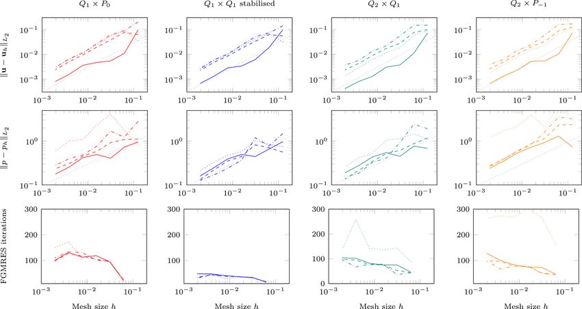
C. Thieulot and W. Bangerth: Q1 × Q1 -stab in geodynamics                                                                         237

Figure 3. Donea and Huerta benchmark. (a) Root mean square velocity as a function of the mesh size h. The dotted line is the analytical
value. (b) Number of FGMRES solver iterations as a function of the mesh size h.

Figure 4. SolCx benchmark. Velocity (a) and pressure (b) fields obtained on a mesh with a resolution of 32 × 32 grid with the Q2 × Q1
element.

   Deubelbeiss and Kaus (2008) thoroughly investigated this           experiments such as the current one that these elements will
problem with various numerical methods (FEM, FDM), with               not yield better convergence orders despite their additional
and without tracers, and conclusively showed how various              cost.
schemes of averaging the density and viscosity lead to differ-           Since harmonic averaging yields the lowest errors we se-
ent results. Heister et al. (2017) also come to this conclusion       lect this averaging and now turn to the pressure field for all
and also considered how averaging the coefficient on each             elements as shown in Fig. 9. We find that the recovered pres-
cell affects the number of iterations necessary to solve the          sures on the line y = 1 follow the analytical solution outside
linear systems. We repeat these experiments here but with our         the inclusion but are less accurate inside the inclusion where
larger set of different elements. Specifically, results obtained      it should be identically zero (Fig. 10).
with no averaging inside the element (“No”), arithmetic av-
eraging (“Arith”), geometric averaging (“Geom”), and har-             5.4   The sinking block
monic averaging (“Harm”) are shown in Fig. 8. We see that
(i) all four elements show the same rate of convergence: O(h)
for velocity errors and O(h0.5 ) for pressure errors; (ii) har-       As discussed in Sect. 4, the stabilized Q1 × Q1 element is
monic averaging always yields lower errors, validating the            sensitive to the choice of a reference density profile as not
findings of Heister et al. (2017); (iii) the number of iterations     only the computed pressure, but also the computed veloc-
in the Stokes solver is the lowest for the stabilized Q1 × Q1         ity field, depends on this choice. This is only relevant for
element; and (iv) this number is not strongly affected by the         buoyancy-driven flows, but because none of the benchmarks
method of averaging (with the exception of the Q2 × P−1 el-           shown previously are driven by buoyancy effects in the pres-
ement). The observation that none of the elements reach their         ence of a background lithostatic pressure to any significant
optimal convergence rate also supports our decision, briefly          degree, let us next consider a setup in which this is the dom-
mentioned in the “Goals of this paper” part of the Introduc-          inant effect. To this end, we perform an experiment based
tion, to not further investigate higher-order Taylor–Hood ele-        on a benchmark similar or identical to the ones presented in
ments Qk ×Qk−1 or Qk ×P−(k−1) with k > 2: we know from                May and Moresi (2008), Gerya (2019), Thieulot (2011), and
                                                                      Schuh-Senlis et al. (2020).

https://doi.org/10.5194/se-13-229-2022                                                              Solid Earth, 13, 229–249, 2022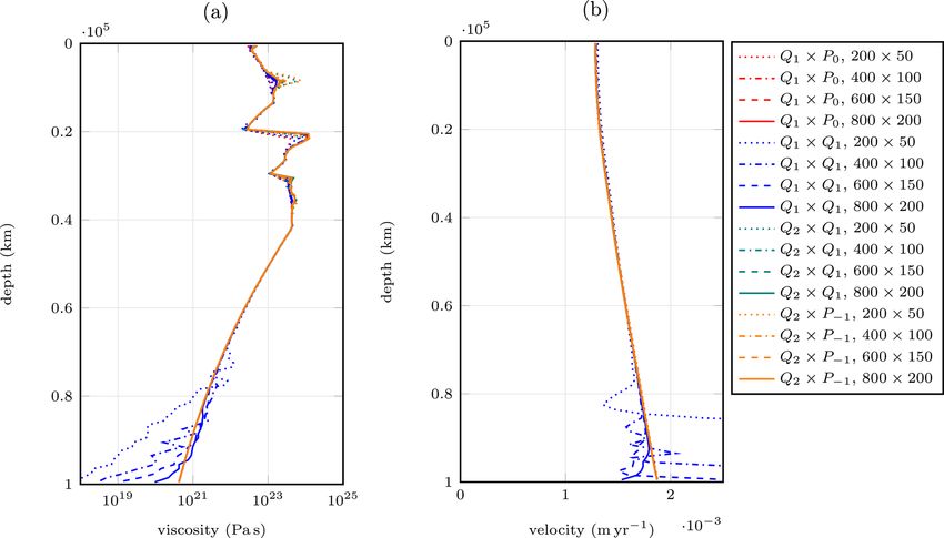
238                                                                  C. Thieulot and W. Bangerth: Q1 × Q1 -stab in geodynamics

Figure 5. SolCx benchmark. Error convergence as a function of the mesh size h. (a) Velocity error; (b) pressure error.

                                                                           In the following, we will denote as Method 1 the approach
                                                                        whereby we do calculations with the density field as specified
                                                                        above. Method 2 consists of a “reduced” density field from
                                                                        which the quantity ρ1 has been uniformly removed so that
                                                                        the block has a density δρ, while the surrounding fluid has
                                                                        zero density. As discussed above, the two choices will result
                                                                        in different pressure but the same velocity fields.
                                                                           We have carried out measurements for all four elements
                                                                        with η? ∈ [10−4 : 106 ] and δρ/ρ1 ∈ {0.25 %, 1 %, 4 %} cor-
                                                                        responding to δρ ∈ {8, 32, 128} kg m−3 . Results for ν =
                                                                        f (η? ) for all elements, the three block density values, and
Figure 6. SolCx benchmark. Number of FGMRES solver iterations           five different mesh resolutions are shown in Fig. 11 for the
as a function of the mesh size h.                                       two methods.
                                                                           When using the full density, we see that all elements, with
                                                                        the exception of the stabilized Q1 ×Q1 element, yield results
    It consists of a two-dimensional 512 × 512 km do-                   which align on a single curve on the plots once sufficient res-
main filled with a fluid (the “mantle”) of density ρ1 =                 olution is reached. We find that measurements pertaining to a
3200 kg m−3 and viscosity η1 = 1021 Pa s. A square block of             given resolution but different δρ are always collapsed onto a
size 128 × 128 km is placed in the domain and is centered at            single line. It is worth noticing that the Q2 ×P−1 element re-
location (xc , yc ) = (256, 384 km) so as to ensure that its sides      sults seem to be the least resolution-dependent. On the other
align with cell boundaries at all resolutions, avoiding cases           hand, the stabilized Q1 × Q1 element yields very anomalous
in which the quadrature within one element corresponds to               results which are orders of magnitude off at all resolutions,
different density or viscosity values. It is filled with a fluid        especially for η1 /η2  1. In addition, we find that for this
of density ρ2 = ρ1 + δρ and viscosity η2 . The gravity vector           element, the value of δρ strongly affects the measurements,
points downwards with |g| = 10 m s−2 . Boundary conditions              as expected based on the discussions in Sect. 4; as a result,
are free-slip onR all sides. The pressure null space is removed         the curves for the same mesh resolution but different δρ2 no
by enforcing  p dV = 0, and only one time step is carried              longer coincide (see Fig. 11b).
out. The benchmark then solves for the instantaneous pres-                 When reduced densities are used results are unchanged
sure and velocity field for this setup.                                 for the stable elements (only Q2 × Q1 results are shown in
    In a geodynamical context, the block could be interpreted           Fig. 11e), and the results for the stabilized Q1 × Q1 results
as a detached slab (δρ > 0) or a plume head (δρ < 0). As                are substantially improved. For values η1 /η2 < 1 we see that
such its viscosity and density can vary (a cold slab has a              all results align on the expected curve, but this is far from
higher effective viscosity than the surrounding mantle, while           true for η1 /η2  1 even at high resolution.
it is the other way around for a plume head). The block den-               In Fig. 12 we show the velocity field in the case η? =
sity difference δρ can then vary from a few to several hun-             10−4 (i.e., the viscosity of the block is 10 000 times smaller
dred kilograms per cubic meter (kg m−3 ) to represent a wide            than the surrounding mantle) and δρ = 8 kg m−3 . When the
array of scenarios. As shown in Appendix A.2 of Thieulot                Q2 × Q1 element is employed in conjunction with Method
(2011), one can independently vary η1 , ρ2 , and η2 and mea-            1 we see in Fig. 12a that the velocity field is strongest in-
sure |vz | for each combination: the quantity ν = |vz |η1 /δρ is        side the block with a maximum value of about 5 mm yr−1 in
then found to be a simple function of the ratio η? = η2 /η1 .           its center. We see that the Q2 × Q1 and Q2 × P−1 elements
At high enough mesh resolution all data points collapse onto            yield nearly identical results (Fig. 12b), so we consider this to
a single line.

Solid Earth, 13, 229–249, 2022                                                                https://doi.org/10.5194/se-13-229-2022
C. Thieulot and W. Bangerth: Q1 × Q1 -stab in geodynamics 239 Figure 7. SolVi benchmark with inclusion of radius 0.2. Velocity (a) and pressure (b) fields obtained on a 256 × 256 mesh using Q2 × Q1 elements. Figure 8. SolVi benchmark. Left to right: Q1 × P0 , stabilized Q1 × Q1 , Q2 × Q1 , and Q2 × P−1 . Top to bottom: velocity error, pressure error, and number of FGMRES iterations for the Stokes solve. The individual lines in each graph correspond to different ways of averaging coefficients on each cell: dotted lines use the correct unaveraged values of coefficients at each quadrature point; dash-dotted lines compute the arithmetic average of the values at the quadrature points on a cell and use the average for all quadrature points; dashed lines use the geometric average; solid lines use the harmonic average. The gray dotted line in the first two rows indicates O(h) convergence for velocity and O(h0.5 ) for pressure. be the correct solution of the physical experiment. The same would probably yield the expected curve, but such resolu- setup with the stabilized Q1 ×Q1 (left half of Fig. 12c) yields tions are intractable in three dimensions and better results can a velocity field that is also maximal in the middle of the block be obtained at much lower resolutions with other elements. but nearly 1000 times larger in amplitude. If we now switch Finally, in Fig. 13 we plot the normalized pressure p ? = to Method 2 (right half of Fig. 12c) the amplitude of the ve- p/(δρ g Lb ) at the center of the block (where Lb is the size locity is reduced by 2 orders of magnitude, but it is still much of the block) as a function of the viscosity ratio η? in the case too large compared to the true solution. in which a reduced density field is used. For the Q2 ×Q1 and These observations illustrate the unreliable nature of the the stabilized Q1 × Q1 elements, the pressure at this point is results obtained with stabilized Q1 ×Q1 elements in the con- uniquely defined since the elements have continuous pres- text of buoyancy-driven flows. Looking at Fig. 11f we see sures. For the other two elements the pressure is discontinu- that increasing the resolution to 512 × 512 or 1024 × 1024 ous across element edges, and it is therefore not uniquely de- https://doi.org/10.5194/se-13-229-2022 Solid Earth, 13, 229–249, 2022
240                                                                   C. Thieulot and W. Bangerth: Q1 × Q1 -stab in geodynamics

Figure 9. SolVi benchmark. Pressure field for the Q1 × P0 , stabilized Q1 × Q1 , Q2 × Q1 , and Q2 × P−1 elements from left to right and
top to bottom at resolution 128 × 128 with no averaging. Note the different color scales, illustrating the differing size of overshoots and
undershoots for the different discretizations.

                                                                         only slowly and, matching the observation in Sect. 5.1, at the
                                                                         cost of not only a fine mesh but also very large numbers of
                                                                         linear solver iterations.
                                                                            In addition to the slow convergence of the Q1 × P0 el-
                                                                         ement, the most striking conclusion of this benchmark is
                                                                         that for buoyancy-driven flows, the solution obtained using
                                                                         the stabilized Q1 × Q1 element on typical meshes not only
                                                                         strongly depends on the choice of the otherwise arbitrary ref-
                                                                         erence density, but is also almost entirely unreliable even on
                                                                         meshes that are already quite fine.

Figure 10. SolVi benchmark. Pressure on the horizontal ray starting
from the center of the inclusion at x = 1.
                                                                         6   Numerical results for a model application

                                                                         While the previous sections have built our intuition for which
fined at our measurement point. We have then chosen to mea-              element may actually work in the context of geodynamics
sure it at four locations corresponding to (xc ± δx, yc ± δy),           applications, they have only done so through abstract and
where δx = δy = 0.1 m, and show the normalized pressures                 idealized benchmarks. It is therefore interesting to investi-
at all four of these locations in the figure. For the Q2 × P−1           gate what one would find in more realistic setups, and conse-
element, the difference between these values is negligible but           quently we have also investigated convergence for a situation
not so for the Q1 × P0 for which the pressure is a stairstep             still sufficiently simple that numerical simulations can reach
function with very different values depending on which step              reasonably high accuracy but that has more of the complex-
an evaluation point is on. The distance between the two lines            ity one would generally find in “real” simulations. Given that
for the Q1 × P0 element decreases with mesh refinement (in-              the previous examples have highlighted the fact that the sta-
dicating convergence of the pressure to the true value), but             bilized Q1 × Q1 element has difficulties with the pressure

Solid Earth, 13, 229–249, 2022                                                                https://doi.org/10.5194/se-13-229-2022
C. Thieulot and W. Bangerth: Q1 × Q1 -stab in geodynamics 241
mation based on dislocation creep flow laws:
−1/n −1+1/n Q + pV
ηdisl = A ε̇ exp , (15)
nRT
where A is a material constant, n is an index typically be-
tween 3 and 4, Q is the activation energy, V is the activation
volume, R the gas constant, T the temperature, and ε̇ is the
effective strain rate (the square root of the second invariant of
the corresponding tensor). Stresses are limited plastically at a
yield stress σy = C cos(φ) + P sin(φ) via a Drucker–Prager
criterion where C is the cohesion and φ the angle of fric-
tion. We use distinct values for some of these parameters in
the initially 20 km thick upper crust (wet quartzite), an ini-
tially 10 km thick lower crust (wet anorthite), and the mantle
(dry olivine), which initially occupies the remaining 70 km
in depth. Deformation is seeded by a weak area within the
mantle lithosphere. We only carry out a single time step as
obtained with a CFL number of 0.5.
A complete and concise description of this setup has more
parameters than are worth spelling out in detail here. For a
detailed description, see Naliboff and Buiter (2015) and the
section of the A SPECT manual along with the corresponding
input files. For the purposes of this paper, the important part
is that both the yield stress and the dislocation creep rheology
depend on the pressure; as a consequence, we can anticipate
that elements that result in poor pressure accuracy may not
yield accurate simulations in general.
Figure 11. Sinking block benchmark. (a–d) ν = |vz |η1 /δρ as a This setup produces localized shear zones that accommo-
function of η? = η2 /η1 as obtained with the four elements with date the majority of the deformation. Figure 14 illustrates
full density; (e, f) same with reduced density for only two element the structure of the resulting solution. Each panel of the fig-
types. Legend: • 16×16 resolution, 32×32 resolution, 64×64
ure shows in its left half the solution produced by the stabi-
resolution, 4 128 × 128 resolution, N 256 × 256 resolution. Colors
represent the element used. For each mesh resolution, we show sep-
lized Q1 ×Q1 element and its right half that produced by the
arate curves for δρ/ρ1 ∈ {0.25 %, 1 %, 4 %}; for all but the stabilized Taylor–Hood Q2 ×Q1 element. Because the solution is sym-
Q1 × Qq element, these curves coincide. Note the different y axis metric, the two halves should be mirror images. It is, how-
used for the stabilized Q1 × Q1 element in (b) and (f). ever, clear from several of the panels that this is not the case:
the Q1 × Q1 element produces large artifacts at depth where
the pressure is large and the pressure dependence of the ma-
terial strong.
approximation, we are specifically interested in a situation in This effect is also demonstrated in a different way in
which the material behavior is pressure-dependent. Fig. 15 where we show laterally averaged quantities for
To this end, we consider an example of continental ex- the different elements and different mesh resolutions. Even
tension here. The setup is similar to ones that can be found though it is clear from Fig. 14 that lateral averaging should
in Huismans and Beaumont (2002), Jammes and Huismans result in a better approximation (than pointwise evaluations)
(2012), Naliboff and Buiter (2015), and Brune et al. (2017), of the correct quantities for a given depth, Fig. 15 shows that
and we specifically use the one that can be found in the “con- even the average is far from correct. On the other hand, the
tinental extension” cookbook of the manual of the A SPECT figure shows that with increasing mesh resolution, the solu-
code (Bangerth et al., 2022). The situation we model here tions produced by the Q1 × Q1 seem to converge to the so-
is characterized by the following building blocks: on a do- lutions generated by the other elements – albeit very slowly
main of size 400 km × 100 km, we impose an extensional and at what one might consider an unacceptable cost.
horizontal velocity component of ±0.25 cm yr−1 on the sides To investigate the origin of these convergence problems of
and a vertical upward velocity of 0.125 cm yr−1 at the bot- the Q1 ×Q1 element, one should recall that the model is non-
tom. The tangential components are left free. At the top, linear. As a consequence, the artifacts may be related to the
we allow for a free boundary. More interestingly, we use a discretization or to a failure of the nonlinear iteration – and
pressure- and temperature-dependent viscoplastic rheology the two may be connected. All of the solutions we show were
of Drucker–Prager type with parameters for viscous defor- taken after 100 Picard iterations to resolve the nonlinearity
https://doi.org/10.5194/se-13-229-2022 Solid Earth, 13, 229–249, 2022You can also read


