National Scale 3D Mapping of Soil pH Using a Data Augmentation Approach - MDPI
←
→
Page content transcription
If your browser does not render page correctly, please read the page content below
remote sensing
Article
National Scale 3D Mapping of Soil pH Using a Data
Augmentation Approach
Pierre Roudier 1,2,∗ , Olivia R. Burge 3 , Sarah J. Richardson 3 , James K. McCarthy 3 ,
Gerard J. Grealish 1 and Anne-Gaelle Ausseil 4
 1   Manaaki Whenua—Landcare Research, Private Bag 11052, Manawatū Mail Centre,
     Palmerston North 4442, New Zealand; GrealishG@landcareresearch.co.nz
 2   Te Pūnaha Matatini, A New Zealand Centre of Research Excellence, Private Bag 92019,
     Auckland 1142, New Zealand
 3   Manaaki Whenua—Landcare Research, P.O. Box 69040, Lincoln 7640, New Zealand;
     BurgeO@landcareresearch.co.nz (O.R.B.); RichardsonS@landcareresearch.co.nz (S.J.R.);
     McCarthyJ@landcareresearch.co.nz (J.K.M.)
 4   Manaaki Whenua—Landcare Research, P.O. Box 10, Wellington 6143, New Zealand;
     AusseilA@landcareresearch.co.nz
 *   Correspondence: roudierp@landcareresearch.co.nz

 Received: 11 August 2020; Accepted: 1 September 2020; Published: 4 September 2020

 Abstract: Understanding the spatial variation of soil pH is critical for many different stakeholders
 across different fields of science, because it is a master variable that plays a central role in many soil
 processes. This study documents the first attempt to map soil pH (1:5 H2 O) at high resolution (100 m)
 in New Zealand. The regression framework used follows the paradigm of digital soil mapping, and a
 limited number of environmental covariates were selected using variable selection, before calibration
 of a quantile regression forest model. In order to adapt the outcomes of this work to a wide range
 of different depth supports, a new approach, which includes depth of sampling as a covariate,
 is proposed. It relies on data augmentation, a process where virtual observations are drawn from
 statistical populations constructed using the observed data, based on the top and bottom depth of
 sampling, and including the uncertainty surrounding the soil pH measurement. A single model
 can then be calibrated and deployed to estimate pH a various depths. Results showed that the
 data augmentation routine had a beneficial effect on prediction uncertainties, in particular when
 reference measurement uncertainties are taken into account. Further testing found that the optimal
 rate of augmentation for this dataset was 3-fold. Inspection of the final model revealed that the most
 important variables for predicting soil pH distribution in New Zealand were related to land cover
 and climate, in particular to soil water balance. The evaluation of this approach on those validation
 sites set aside before modelling showed very good results (R2 = 0.65, CCC = 0.79, RMSE = 0.54),
 that significantly out-performed existing soil pH information for the country.

 Keywords: digital soil mapping; soil pH; data augmentation; quantile regression forest

1. Introduction
      Soil pH indicates the relative acidity or alkalinity of the soil, and is a master variable in soil science,
both in managed and un-managed landscapes [1]. It plays a central role in numerous soil functions,
soil quality, and fertility processes, impacting on physical structure, carbon, nitrogen, and phosphorus
cycling, biological activity and regulation, bioavailibility of a range of nutrients, mobility and uptake
of some trace elements such as cadmium [2,3]. This translates to soil pH being a parameter that
is critical for a wide range of applications and stakeholders, such as the fertiliser industry, the soil

Remote Sens. 2020, 12, 2872; doi:10.3390/rs12182872                         www.mdpi.com/journal/remotesensing
Remote Sens. 2020, 12, 2872                                                                           2 of 22

ecology community, and soil quality initiatives. Freshwater wetlands can be classified according to
their edaphic properties [4], with pH being one of the key elements distinguishing wetland classes
such as bogs and marshes. Land use evaluation is another application where soil pH is an important
proxy for toxicity or sufficiency of nutrients [5]. As soil pH is spatially variable, it has been used as a
spatial input layer to assist mapping wetland types [6], or crop suitability [7,8]. Soil pH has also been
identified as one of the key indicators for monitoring soil quality [9,10] and soil security [11].
      In New Zealand, spatially explicit soil pH estimates are mostly available through one of
the Fundamental Soil Layers (FSL [12]). The FSL is a polygon-based soil information product.
It was developed across 30 years from a combination of stereoscopic analysis of aerial photographs,
pedological knowledge, and field verification. The coverage is consistent across most of the country,
at a nominal scale of 1:50,000, although it does not provide estimates for Stewart Island/Rakiura.
For each of the 100,000+ polygons, an estimated modal soil pH value was interpreted by pedologists
familiar with the region, based either on previous soil surveys or on landscape analysis. The soil depth
corresponding to those pH estimates is the 20–60 cm interval. FSL is widely regarded as outdated
and inaccurate by soil scientists, but is still commonly used across the country. The other soil pH
product currently available for New Zealand is SoilGrids [13], which used digital soil mapping (DSM)
to map soil pH at the global scale. The SoilGrids predictions are generated at a resolution of 250 m,
and for six different depth intervals. So far, no formal comparison has been made between the FSL
and SoilGrids products specifically for New Zealand, but studies in other countries suggest that a
national DSM model, trained using local data, could provide more accurate results than the global
model used by SoilGrids [14].
      Most of the methodologies in the DSM literature use a combination of individual models,
that are fitted for different fixed depth intervals, covering different parts of the soil profile. Typically,
the standard set of six depth intervals proposed by the GlobalSoilMap initiative [15] are used.
Before modelling, the depth support of the point observations are generally changed to these depth
intervals using the mass-preserving spline function proposed by Bishop et al. [16]. This so-called
2.5D approach is prevalent in the literature; however, 3D methods, which take the depth dimension
into account more explicitly, have been proposed more recently, and acknowledge the true three
dimensional nature of the soil [17]. Earlier attempts to represent the variation of soil properties with
depth were hand-drawn depth functions and indicatrix [18]. Quantitative approaches were then
developed, and included the use of exponential decay [19], and peak [20] functions to statistically
produce a continuous representation of soil properties down the soil profile. Malone et al. [21] used
the mass-preserving spline proposed by Bishop et al. [16] after a 2.5D DSM modelling exercise to
re-construct the predicted values for a suite of different soil depth intervals.
      Soil depth is a parameter that is easy to measure, and impacts most if not all soil properties,
due to its tight links with a range of pedogenetic processes [18]. In order to include the depth support
of the observed data into the final model, Orton et al. [22] proposed a 3D area-to-point kriging
method. More recently, several authors have suggested using specific points in the sampled horizons
(often, the mid-point of the horizon) to include depth as covariate [13,23,24]. Brus et al. [25] also tested
using soil depth as a covariate in a small region of China, both as a continuous or as a categorical
variable. They found that those 3D models were outperformed by 2.5D models fitted on the same
dataset. Nauman and Duniway [26] compared 3D and 2.5D approaches in the upper catchment of the
Colorado River in the United States of America. They found that the best model would often depend
on the characteristics of the soil attribute modelled, and that 3D models, while out-performing 2.5D
models for some attributes, could exhibit larger prediction uncertainties.
      Using a single 3D model with soil depth as a covariate presents several advantages, the model can
be fitted across the wide range of sampled depths present in the soil pH database, which removes the
need to harmonise the depth support of the measurements present in the database prior to modelling.
While the mass-preserving spline approach proposed by Bishop et al. [16] has been widely applied,
there are associated issues with its use, such as the automated handling of abrupt property changes
Remote Sens. 2020, 12, 2872                                                                          3 of 22

across very distinct horizons, or the inclusion of uncertainties affecting the observations. The other
advantage of a 3D approach is that the final predictions can be dynamically re-aggregated in different
soil depth supports (for example, to serve the needs of different stakeholders) without having to re-fit a
different model. In the case of New Zealand, this is an important advantage, as the soil grids produced
using DSM need to address the needs of a variety of stakeholders who use different soil depths in
their analyses.
      The objectives of this study were to (1) calibrate a soil pH DSM model for New Zealand that
uses the best set of observations available for the country; (2) test the potential of a novel 3D DSM
approach that augments the amount of depth and attribute information using a resampling strategy;
(3) evaluate the results of this model with those of a more traditional 2.5D approach; and (4) compare
the accuracy of our model against existing soil pH products available for New Zealand.

2. Materials and Methods

2.1. Study Area
     The study area is the terrestrial land mass of New Zealand. Three main islands make up most New
Zealand: North Island/Te Ika-a-Māui, South Island/Te Waipounamu, and Stewart Island/Rakiura.
The latter represents a significant area (1683 km2 ); however, it is very sparsely populated, and is mainly
covered in conservation land. Due to the lack of data coverage, smaller islands and archipelagoes,
such as the Chatham Islands Group, located 800 km east of South Island/Te Waipounamu, and the
sub-Antarctic islands such as the Auckland Islands, were excluded from this study.

2.2. Data
     The approach used to map soil pH at national level follows the paradigm of digital soil
mapping (DSM [27]), which relates point observations of soil properties with environmental
variables representing soil-forming factors [18]. DSM has become a major framework in the
generation of new soil information grids, often underpinned by national or international initiatives
such as GlobalSoilMap [15].

2.2.1. Soil pH Data
     Soil pH data were collated by merging a variety of disparate datasets from a wide range
of soil surveys, soil quality programmes, wetland monitoring programmes, and soil biodiversity
research programmes. The primary dataset was sourced from the National Soil Data Repository
(NSDR, n = 5874, [28]). Soil pH in the NSDR was measured indifferent solutions: in calcium chloride
(CaCl2 ), in water at a 1:5 ratio, and in water at a 1:1 ratio. All pH measurements were converted to soil
pH measured in a 1:5 water solution using a pedo-transfer function based on a simple linear model [29].
The spatial distribution of samples in the NSDR is biased towards productive land, so additional
soil pH data were sourced from a plot-based national survey of forests and shrublands [30], and a
series of site-specific studies in forest ecosystems around New Zealand. These datasets are hereafter
collectively referred to as the “Forests” dataset (n = 3576). Additional points were sourced from the
wetlands soils monitoring program (“Wetlands”, n = 850). Finally, soil pH data were also collated
from Topoclimate South, an intensive soil survey program that took place across the Southland region
(n = 1644). The statistical distribution of soil pH was inspected in order to detect potential outliers.
Samples with pH lower than 2 or higher than 11 were removed from the dataset, as such values were
considered unrealistic for New Zealand conditions.
     The spatial coverage of the point dataset for 1:5 H2 O soil pH (Figure 1) shows that most regions
of New Zealand were well covered by the collated dataset. There were several exceptions: the region
of Canterbury, on the East Coast of the South Island, was poorly covered. However, these are mostly
recent soils, formed on Quaternary gravels, which typically show a lower magnitude of spatial
variation. In the North Island, the most notable data gaps were located in the lower East Coast, in the
Remote Sens. 2020, 12, 2872 4 of 22
regions of Hawke’s Bay and Wairarapa. For the deeper layers, the bias against conservation land was
evident, because samples from the “Forests” and “Wetlands” were collected only in the first 10 cm.
0−5 cm 5−15 cm 15−30 cm
35°S
40°S
45°S
0 250 500km 0 250 500km 0 250 500km
30−60 cm 60−100 cm 100−200 cm
35°S
40°S
45°S
0 250 500km 0 250 500km 0 250 500km
170°E 175°E 180° 170°E 175°E 180° 170°E 175°E 180°
Provenance Forests NSDR Topoclimate South Wetlands
Figure 1. Point data used to model soil pH. The dataset was collated from four different data sources:
the forest soils dataset, the national soil data repository (NSDR), Topoclimate South, and the wetlands
monitoring programme.
A suite of 498 soil profiles (representing 1,520 individual samples) were set aside from the soil
pH dataset before any model calibration, in order to evaluate the predictions of the different models
tested in this study. They are hereafter referred to as the validation set, as opposed to the calibration
set. Entire soil profiles were set aside for validation, in order to account for the autocorrelation of
soil pH observations within soil profiles. Soil profiles in the validation set were selected by using
spatially balanced sampling, as implemented by the pivotal method [31] using the BalancedSampling
R package [32]. All available sites were given the same probability to be included in the validation
set. The selected samples were balanced spatially, but also against the average pH value within
each soil profile.
2.2.2. Environmental Covariates
A large number of spatial layers (n = 29) were pre-selected as potential covariates for soil pH
modelling. They were initially selected on expert basis, following the assumption that all these layersRemote Sens. 2020, 12, 2872 5 of 22
could provide a certain degree of control of soil pH at the national scale. The different layers are listed
on Table 1, and are organised following the common conceptual frameworks that are SCORPAN [27]
and CLORPT [18]. Some of the covariates, such as rainfall or erosion yield, represent direct observations
of a specific soil-forming factor, while others, such as latitude or northerness, represent a proxy for a
wider range of soil-forming factors. The covariate data were processed in SAGA GIS [33] and GRASS
GIS [34], then collated and interpolated to a common grid in GRASS GIS. The final resolution of the
prediction grid was 100 m, and uses the New Zealand Transverse Mercator 2000 projection system.
Finally, as no reliable model of soil depth is available for New Zealand, the SoilGrids layer “depth to
bedrock” [13] was used to censor the depth of soil pH predictions.
Table 1. Covariates short-listed for soil pH modelling.
Name Original Scale/Resolution Reference/Formula
Climate
Mean annual evapotranspiration 2005–2014 500 m Running et al. [35]
Mean annual water deficit 1950–1980 25 m Leathwick et al. [36]
Mean annual rainfall 1972–2014 5110 m Tait et al. [37]
Mean annual temperature 1950–1980 25 m Leathwick et al. [36]
Monthly water balance 25 m Leathwick et al. [36]
Potential evapotranspiration deficit 1972–2014 5096 m Porteous et al. [38]
Annual global solar radiation 25 m Neteler and Mitasova [34], Hofierka et al. [39]
Organisms
Mean annual net primary production 2005–2014 500 m Running et al. [35]
Land cover (2012) 1:50,000 Landcare Research [40]
Potential vegetation 100 m Leathwick [41]
Landscape position
Elevation 25 m Landcare Research [42,43]
Aspect 25 m Neteler and Mitasova [34]
Northerness 25 m cos( aspect) [34]
Easterness 25 m sin( aspect) Neteler and Mitasova [34]
Latitude 25 m Neteler and Mitasova [34]
Distance from coast 25 m Neteler and Mitasova [34]
Relief/Topography
Distance from drainage channels 25 m Olaya and Conrad [33]
Multi-resolution valley bottom floor (MRVBF) 25 m Olaya and Conrad [33]
Multi-resolution ridge top floor (MRRTF) 25 m Olaya and Conrad [33]
Normalised height 25 m Olaya and Conrad [33]
SAGA wetness index (SWI) 25 m Olaya and Conrad [33]
Slope 25 m Neteler and Mitasova [34]
Slope height 25 m Olaya and Conrad [33]
Standard height 25 m Olaya and Conrad [33]
Topographic position index (TPI) 25 m Olaya and Conrad [33]
Valley depth 25 m Olaya and Conrad [33]
Wind exposition index 25 m Olaya and Conrad [33]
Underlying geology and erosion
New Zealand Land Resources Inventory 1:50,000 Landcare Research [44]
Peat 1:50,000 Minasny et al. [45]
2.3. Depth as a Covariate Using Data Augmentation
In statistics, data augmentation refers to the artificial augmentation of the number of observed
data points in order to improve the analysis of the dataset [46]. The augmented dataset is a simulated
dataset, and the augmentation procedure makes use of the characteristics of the observed dataset used
to generate it. This concept has been recently adapted to machine learning, when a suite of subtle
variations to the original dataset are used to increase the size of the calibration set, and improve the
robustness of the generated models [47]. Data augmentation is typically used when the calibration set
presents some deficiencies that might otherwise impair the analysis (missing values, few samples),
or when it does not represent enough variability, and could therefore produce biased results. Here we
propose a method using data augmentation to more rigorously include (i) soil depth as an explanatory
variable, and (ii) soil pH measurement uncertainties in the pH prediction model.Remote Sens. 2020, 12, 2872 6 of 22
2.3.1. Augmenting Depth Information
In soil databases, soil depth is usually recorded using the top and the bottom of the sampled
horizon. Most 3D DSM models published to date take the horizon mid-point as a depth
measurement [13,26]. Here, we improve on this by explicitly acknowledging that these measurements
correspond to material sampled over a depth interval, as opposed to a specific point. The soil pH
measurements in our dataset have been made on samples extracted using a variety of methods,
including coring, augering, or pit sampling, and most have been collected from pedological
horizons—either pedogenetic or functional horizons. An implicit assumption in those cases is that the
sample collected for a given horizon (along with its associated measurements) is representative of all
depths contained in this horizon. Thus, we propose that for a given horizon bounded by the depths
top and bottom, a k-fold data augmentation of the soil depth can be achieved by randomly sampling k
values from a uniform distribution U (min, max ), where min and max are the top and bottom depths of
the horizon (Figure 2a).
2.3.2. Augmenting Attribute Information
Data augmentation can also aim at improving the representativeness of the dataset used to
calibrate a predictive model, and better represent the subtle variations that exist in the real world
phenomena that are being modelled. In our case, we propose to include information about the
uncertainty in soil pH measurement in the way the soil pH values are included in the different
augmented datasets. In the absence of a more accurate alternative, we propose that the soil pH
measurement associated with a given horizon can be described by a normal distribution N (µ, σ ),
where µ is the measured pH value for that horizon, and σ is a standard deviation describing the
uncertainty of the pH measurement method (Figure 2b). Replication analysis at the laboratory
responsible for most of our measurements (Manaaki Whenua—Landcare Research Environmental
Chemistry Laboratory, Palmerston North, New Zealand) suggest that this standard deviation would
be around 0.1.
Combining the augmentation of depth and soil pH information allows to convert the original
dataset (Figure 2c, left) into a k-augmented, virtual dataset (Figure 2c, right). While Figure 2c shows a
4-fold data augmentation, the effects of using different values of k have been tested in this study.
2.4. Modelling Framework
In this study, random forest (RF [48]) was the main tool used at different steps of the modelling,
i.e., for feature selection of the final soil pH predictors, and then to calibrate the soil pH prediction
model. A RF is an ensemble of regression trees that have been generated through bootstrapping.
For a regression problem, a large number of decision trees are generated (the “forest”, with a number
of trees ntrees between 500 and 2000 typically being grown for most RF applications). Each tree
is generated from an independent bootstrap of the calibration dataset, until the size of the nodes
reaches a minimum size limit (node size). Unlike other similar algorithms, no pruning is done on the
trees, however, at each node of the trees, a random subset of the available predictors (of cardinality
mtry, where mtry ≤ n and n is the number of predictors) is chosen. The default value of mtry is
√
arbitrarily chosen as n or n/3 by most RF implementations, but it is a parameter which, like node
size, needs hyper-parameterisation [49]. Finally, every tree generates an individual prediction, and the
RF prediction is an average of all individual tree predictions. In that sense, RF is considered an
ensemble model. Samples left out by the bootstrap sampling are used to evaluate the predictions of
each tree, and are referred to as “out-of-the-bag” (OOB).Remote Sens. 2020, 12, 2872 7 of 22
4
1
2
=
...
=
=
k
k
k
0
6.36
15
5.91
30
5.81 μ
60
75 σ
depth (cm)
5.08
140
170
4.53
200
6.36 pH
227 6.38 6.58
6.30 6.43
(a) (b)
site depth ph
SB08459 3 6.43
SB08459 7 6.38
SB08459 10 6.30
SB08459 14 6.58
SB08459 16 5.89
SB08459 22 5.77
SB08459 24 5.96
site top bottom ph
SB08459 29 5.79
SB08459 0 15 6.36
SB08459 33 5.98
SB08459 15 30 5.91
SB08459 45 5.84
SB08459 30 60 5.81
SB08459 52 5.86
SB08459 75 140 5.08
SB08459 59 5.72
SB08459 170 227 4.53
SB08459 83 5.29
SB08459 86 5.03
SB08459 102 5.12
SB08459 131 5.09
SB08459 178 4.38
SB08459 182 4.54
SB08459 189 4.44
SB08459 196 4.56
(c)
Figure 2. Data augmentation of both depth and attribute information contained in the observation
data set. (a) k-fold data augmentations of soil depth (k = 1, 2, and 4 respectively). Note that for k = 1,
soil depth is a single value picked randomly between the top and bottom depths of each horizon in
the dataset. (b) 4-fold data augmentation of a soil pH measurement. Four different values (in dark
green) are sampled from a normal distribution of mean µ, the measured pH value, and of standard
deviation σ, whose value is estimated by the expert. (c) 4-fold data augmentation of the observed data
of a soil profile containing five horizons.
The RF implementation used throughout the analysis was ranger [50], which is computationally
efficient and easily parallelisable. To generate the final pH predictions, the quantile regression forest
method was used (QRF [51]). QRF infers conditional quantiles by generalising the RF algorithm to
conditional distributions (as opposed to just the mean), and therefore can derive prediction intervals,
along with a median prediction [52]. All modelling was done in R version 3.6.3 [53].
2.4.1. Variable Selection
The number of environmental covariates selected for soil pH modelling was substantial,
and numerous variables presented significant levels of correlation. While there was discussionsRemote Sens. 2020, 12, 2872 8 of 22
on the ability of RF to handle a large number of correlated variables, and while the environmental
covariates have been pre-selected using expert knowledge about the soil-forming factors associated
with soil pH differences across New Zealand, the choice was made in this study to use variable selection
to restrict the number of input variables, and combine the performance of RF with the interpretability
of a parsimonious model [54,55].
The variable selection approach used was Variable Selection Using Random Forests (VSURF) [56],
as implemented in the eponymous package for R [57]. The VSURF approach works in two steps,
corresponding to two different, but complementary, goals. The first step aims at finding all the
important variables for interpretation, even where there is redundancy within the selected set of
variables. The second step reduces the number of variables further, and aims to restrict the predictors
to a parsimonious suite of important variables, avoiding redundancy so as to get the best prediction
model possible. The VSURF algorithm uses an iterative procedure with ranking and permutation of
the variables in a large number of RF runs. The ranking itself is done based on the mean OOB error
rate, defined as the sum of squared errors:
1
errOOB =
n ∑ (yi − ŷi )2 (1)
i ∈{1,...,n}
where ŷi is the predicted value of yi by trees belonging to the OOB samples.
We used repeated 10-fold cross-validation (with 30 repeats) to find the optimal parameters for
the RF with all the potential environmental predictors in order to determine which parameters to use
with VSURF. The set of parameters minimising the root mean squared error (RMSE) were mtry = 6
and node size = 5. Following Genuer et al. [56], the number of trees in the RF was set to ntree = 2000,
since using RF for variable selection requires more trees than the number typically used in regression
so to give stable results [49].
2.4.2. Calibration of the Soil pH Model
A predictive model for soil pH from the selected variables was calibrated for different values of
the augmentation factor (k ∈ {2, 3, 4, 5, 6, 7, 8, 10}) and different levels of uncertainty associated with
the reference soil pH measurement (σ ∈ {0, 0.01, 0.05, 0.1, 0.15, 0.20, 0.25, 0.30}), in order to test the
effects of these two factors. Additionally, strategies of (i) taking the mid-point of the horizon depths,
and (ii) using a random depth between the top and the bottom of each horizon (which corresponds to
k = 1) were also tested.
The hyper-parameterisation of each model (mtry and node size) was done on the calibration
set using repeated spatial cross-validation using the CAST package [58] with 10 folds and 50 repeats.
Spatial cross-validation was used in order to avoid the impact of spatial auto-correlation during the
cross-validation [55]. The number of trees per forest was set to ntree = 500, since using more trees did
not improve the accuracy of the model (results not shown), and following the suggestion that using
too many trees might be detrimental in some cases [49]. Optimal hyper-parameters of the models were
chosen to minimise the root mean square error (RMSE).
Soil pH predictions were then generated for the 100-m resolution grid supporting the
environmental covariates. The optimal prediction model was used to develop predictions for each
centimetre of soil depth between 0 and 200 cm (depth ∈ {0, 1, . . . , 200 } cm). The median predictions
of soil pH were generated alongside the 5th, 25th, 75th, and 95th quantiles, so that the 50% and 90%
prediction intervals could be calculated. Finally, maximum soil depth was used to prevent producing
any values deeper than the depth to bedrock. The maximum soil depth estimates from SoilGrids
250 m [13] were used as there is currently no such national estimates for New Zealand.Remote Sens. 2020, 12, 2872 9 of 22
2.5. Evaluation and Comparison to Existing Products
The generated soil pH maps were inspected visually for consistency with what is known in
terms of soil pH distribution across New Zealand soils [59,60]. Then, the validation sites were
used to evaluate the performance of the pH predictions, and compared with the other existing
information products covering New Zealand: the soil pH layer from the Fundamental Soil Layers
(FSL [12]), and SoilGrids 250 m [13]. The proposed approach was also compared with the more
common 2.5D DSM approach, which involves (i) harmonising the observed soil data to predefined
depth intervals using a mass-preserving spline, then (ii) fitting an independent prediction model
for each of these depth intervals. The GlobalSoilMap intervals were used as the predefined depth
intervals, since they are the de facto standard for this type of soil information product, and cover the
entire soil profile [15]. Our calibration soil pH data were splined using the methodology originally
proposed by Bishop et al. [16] to fit the six standard GlobalSoilMap depths. Then, at each depth
interval, a predictive model was calibrated using the methodology presented above—but excluding
soil depth from the covariates.
The respective predictions of both methodologies were aggregated back to the original depth
support of the validation samples. To do so, soil pH estimates were re-aggregated on the depth support
used by the different validation profiles. The integration method detailed in the following section
was used to adapt the soil pH of our approach, while results from the 2.5D DSM approach, FSL and
SoilGrids predictions were adapted using weighted averaging based on 1 cm slices, using the method
of Beaudette et al. [61]. Performance metrics were then computed by comparing the predicted and
observed values for the different approaches and products: R2 , RMSE, bias, and Lin’s Concordance
Correlation Coefficient (CCC).
2.6. Adaptation of the Predictions to Suit Different End-Users
The dynamic re-aggregation of predictions to tailor the needs of different stakeholders was
demonstrated for different end-users: (i) the GlobalSoilMap project, that uses a set of six standard
depth intervals (depth intervals {0–5, 5–15, 15–30, 30–60, 60–100, 100–200} cm [15]); (ii) the New
Zealand fertiliser industry, which uses a single {0–7.5} cm depth interval; and (iii) both the soil ecology
community and the New Zealand soil quality reporting system, that uses a {0–10} cm depth interval.
To aggregate the pH value Qk , corresponding to the kth quantile estimate for a given horizon H,
bounded by the depths dtop and dbottom , the following formula was used:
R dbottom
dtop qk (dtop , dbottom )
Qk (dtop , dbottom ) = (2)
dtop − dbottom
where qk (dtop , dbottom ) is the depth profile of predicted soil pH, generated using a linear interpolation
of the predicted pH values estimated every centimetre between dtop and dbottom . This approach was
used to aggregate the {5th, 25th, 50th, 75th, 95th} quantiles predicted using QRF.
3. Results
3.1. Soil Data
The summary statistics of the data collated across New Zealand (n = 11,944) for the study
are presented in Table 2. In order to showcase more clearly the impact of soil depth on soil pH,
horizon depths were classified using the GlobalSoilMap depth intervals using a majority rule.
Generally, soil pH increases with depth, with the 0–15 cm interval (corresponding to topsoil in
most NZ regions) being more acidic (mean soil pH < 5 in the upper 15 cm, and >5 below 15 cm).
Many samples (almost half the total number of samples) were collected in the top 15 cm, which again
is explained by past studies that have focused on the uppermost horizons (the forest and wetlands data
in particular). The number of samples available past 100 cm depth was much smaller (884 samples,Remote Sens. 2020, 12, 2872 10 of 22
representing 7.4% of the total number of samples), and the deepest samples (past 200 cm) were very few
(52 samples, representing 0.43% of the total number of samples). The observed variability, as assessed
by the inter-quartile range (IQR), shows the 100–200 cm horizon to be the most variable, which can be
explained by the differences in parent material that contribute to variations deeper in the soil profile.
The topsoil depths (0–15 cm) also show a pronounced variability. Skewness of the data was small,
and the data did not require transformation prior to modelling.
Table 2. Descriptive statistics of soil pH (1:5 H2 O), and a break-down of the statistics for the six
GlobalSoilMap depth intervals. N: number of samples. Min.: minimum. Qn : nth quantile. Max.:
maximum. IQR: inter-quartile range. Skew.: skewness.
Depth N Min. Q5 Q25 Mean Median Q75 Q95 Max. IQR Skew.
0–5 cm 2,297 3.04 3.73 4.11 4.72 4.60 5.23 6.08 8.12 1.12 0.75
5–15 cm 2,997 3.04 3.80 4.20 4.86 4.80 5.40 6.16 8.12 1.20 0.51
15–30 cm 1,660 3.30 4.30 5.20 5.53 5.60 5.91 6.46 8.30 0.71 −0.02
30–60 cm 2,296 2.74 4.53 5.20 5.64 5.63 6.09 6.70 8.98 0.89 0.29
60–100 cm 1,810 2.58 4.60 5.24 5.78 5.70 6.20 7.20 9.30 0.96 0.75
100–200 cm 831 3.07 4.60 5.20 5.92 5.70 6.50 8.01 9.30 1.30 0.76
>200 cm 52 4.35 4.77 4.99 5.57 5.40 6.09 6.74 7.80 1.10 0.75
All depths 11,944 1.48 3.90 4.63 5.29 5.30 5.85 6.70 9.30 1.22 0.41
3.2. Selected Predictors and Variable Importance
After the two steps of the VSURF variable selection algorithm, 13 covariates (out of 29) were
retained for modelling. Figure 3 shows the variables selected by the algorithm, sorted by their
respective average OOB error rate. The most important covariate for prediction was land cover,
followed by covariates related to moisture status (potential evapotranspiration, annual water deficit,
monthly water balance, mean annual rainfall). This was not surprising, because the relationships
between both land cover and soil-water balance with soil pH are well documented [9,62,63]. Then,
soil depth and latitude were also selected. Position within the soil profile has an obvious impact on
soil pH (Table 2), with the impact of water flows and various organisms being more pronounced near
the surface. Latitude, on the other hand, is a compounding factor: due to the shape of New Zealand,
which spans from sub-tropical latitudes (32◦ ), down to latitudes nearing 50◦ on Rakiura/Stewart Island,
latitude encompasses a range of climatic effects. The last group of selected variables is composed of
terrain variables (elevation, SAGA wetness index), climatic variables (solar radiation, mean annual
temperature, observed evapotranspiration), and biological input (net primary production).
The absence of parent material information in the final model is surprising, but the quality
of the main source of parent material information (the “top rock” field of the New Zealand Land
Resource Inventory, [44]) is limited, and work is currently underway to better represent the pattern
of parent material across New Zealand. Moreover, other variables, such as latitude, and climatic
factors, such as rainfall and temperature, might be already capturing the spatial patterns of parent
material (e.g., volcanic material in the north of the country, Quaternary gravel deposits in the south).
Further inspection of the covariates shows strong correlations between parent material and land cover,
or potential evapotranspiration, for example. As for all data-driven DSM exercises, care should be
taken when trying to infer knowledge about the drivers of soil properties solely from an analysis of
variable importance [64]. Variables were selected and used by the model in order to produce the best
possible prediction, and the model does not reflect their relative importance in terms of soil processes.
It also does not distinguish whether selected variables are impacting soil pH, or affected by soil pH.Remote Sens. 2020, 12, 2872 11 of 22
0.5
0.4
Mean OOB error rate
0.3
0.2
0.1
0.0
er
ET
e
th
n
Ba it
ce
n.
p.
P
x
.
ET
ad
de
ic
ud
io
l S NP
m
ep
ai
ov
an
ef
at
R
t.
d
In
R
Te
tit
C
D
D
Po
ve
ev
l
d
ar
La
al
t.
ve
nd
al
er
El
er
ea We
ol
nu
nu
er
at
er
La
bs
An
lW
at
An
bs
A
O
ba
W
G
O
n
n
a
n
lo
SA
ea
nu
ly
ea
n
G
ea
th
M
An
M
M
t.
on
M
Po
M
Variable
Figure 3. The final set of covariates retained by the VSURF prediction step, and their mean contribution
to the out-of-the-bag (OOB) error rate. Explanatory variables with high mean OOB error rates have
more impact on the model. Pot. ET: Potential evapotranspiration. Mean Annual Rain.: Mean Annual
Rainfall. Mean Annual Temp.: Mean Annual Temperature. Mean Observed NPP: Mean observed
net primary production. Pot. Global Solar Rad.: Potential global solar radiation. SAGA Wet. Index:
SAGA wetness index. Mean Observed ET: Mean observed evapotranspiration.
3.3. Impact of Data Augmentation on Predictions
Figure 4 shows the impact of (i) the data augmentation strategy and (ii) the magnitude of
the uncertainty of the pH measurement technique on the performance of the model. Results are
shown both on the OOB samples, which are set aside during the RF training, and on the validation
samples. On the OOB samples, and with low uncertainty around the pH values used for modelling,
data augmentation was beneficial, up to about 5-fold, from which there was no marginal gain. However,
when uncertainties around pH values in the calibration set increase over 0.1, data augmentation was
optimal around a 3-fold augmentation rate, after which the benefits of augmentation on RMSE
were more limited, but still yielded better results than no augmentation. There was no difference
between the mid-point and the random depth strategies in terms of OOB RMSE. On the validation set,
data augmentation was not beneficial compared with no augmentation when pH uncertainties were
either very low or ignored. For pH uncertainties over 0.1 however, it was beneficial on validation RMSE,
up to a level of 3-fold, from which no marginal gains were observed. Following these observations,
an augmentation rate of k = 3 was used for the rest of the modelling, along with the standard deviation
of pH values σ = 0.1 that was provided by the laboratory processing our datasets.
3.4. Model Evaluation
Results for the 498 soil profiles set aside for validation (n = 1520 samples) were used to assess
the pH prediction performance. Overall, the validation statistics showed that the model performed
well (R2 = 0.65, CCC = 0.79). The RMSE of the model across all depths was 0.54. Moreover, the model
showed negligible bias (bias = −0.03). The distributions for predicted and observed pH values
(compared in Figure 5a) showed very minor differences. Most of the divergences between both
distributions occurred around the 90% quantile, and suggest some under-prediction of the highest pH
values. However, the 95% confidence intervals of the distributions were still overlapping, showing
this had minor effects on the overall distribution.Remote Sens. 2020, 12, 2872 12 of 22
Analysis of model residuals showed that they were normally distributed for most validation
sites, and no significant trend could be detected (red line, Figure 5b). Heavy tails on the Q-Q plot
(presented Figure 5c) and a slight deviation from normality can be noted on the Q-Q plot of those
residuals, though. This confirms what was observed in Figure 5a, and this deviation from normality
corresponds to the most alkaline soils (pH > 7). Such alkaline soils, however, are rare in New Zealand,
and represent less than 2% of the measurements that were collated for this study.
OOB
0.30
0.25 pH uncertainty
(standard deviation)
0.3
0.20
RMSE
Validation 0.2
0.57 0.1
0.56
0.0
0.55
0.54
ra int
om
3− d
4− d
5− d
6− d
7− d
8− d
9− d
10 ld
d
l
l
l
l
l
l
l
ol
fo
fo
fo
fo
fo
fo
fo
fo
o
−f
nd
2−
−p
id
m
Augmentation
Figure 4. Influence of the data augmentation strategy and of the magnitude of the pH uncertainty
on the uncertainty of the model predictions. Results are shown for both the OOB samples, and the
validation samples.
a
Observed Predicted
1.0
0.9
Cumulative probability
0.8
0.7
0.6
0.5
0.4
0.3
0.2
0.1
0.0
3 4 5 6 7 8 9
pH
b c
Model residual quantiles
2 2
1 1
Residuals
0 0
−1 −1
−2 −2
4 5 6 7 8 −2 0 2
pH (predicted values) Theoretical normal quantiles
Figure 5. Evaluation of the model’s performance. (a) Cumulative probability function of predicted and
observed pH values. The shaded area surrounding the functions shows their 95% confidence calculated
using Kolmogorov-Smirnov’s D. (b) Residual plot for the model residuals, on the validation samples,
with the red line showing the best linear fit. (c) Normal quantile-quantile plot for the model residuals,
on the validation samples, with the red line showing a normal fit.Remote Sens. 2020, 12, 2872 13 of 22
3.5. Generated Products
3.5.1. Depth Profiles
Depth profiles were generated for 20 validation sites, at a 1-cm resolution from the soil surface,
down to 2 m, or maximum recorded soil depth—whichever occured first (Figure 6). These profiles
were picked at random from validation sites that had more than six horizons sampled, so as to better
study how the model performed throughout the whole profile. Uncertainty of predictions is shown
using the 50% (dark blue band) and 90% (light blue band) prediction intervals, which surround the
median prediction (dark blue line). The reference laboratory measurements are shown in red, and are
surrounded by their 90% confidence interval (red band). Some profiles showed excellent results,
and the prediction does follow the measured pH values, with narrow prediction intervals surrounding
the predictions (e.g., SB08337, SB09355, SB09799). Other examples do follow the reference pattern of
values as they evolve with depth, but present much wider prediction intervals (SB07653, SB09446).
For some profiles, prediction intervals get to a width that make it difficult to use, such as SB09897,
although these do carry useful information from a modelling perspective. Predictions for profiles such
as SB08730 and SB09377 are unsatisfactory: in these specific cases, they correspond to profiles located
in dry climate regions that are less represented in the original datasets. However, most of the inspected
profiles did present a good result.
3.5.2. Maps
Figure 7 shows the pH product aggregated for three different depth intervals that are often
used for topsoil: 0–5 cm (first GlobalSoilMap depth interval), 0–7.5 cm (widely used by the fertiliser
industry in New Zealand), and 0–10 cm (used for national reporting on soil quality in New Zealand,
and widely used by the ecological research community). The differences between these maps are small,
with absolute differences mostlyRemote Sens. 2020, 12, 2872 14 of 22
{7C223A... SB07653 SB08337 SB08471 SB08730
0
50
100
150
200
SB08943 SB09213 SB09214 SB09355 SB09377
0
50
100
150
Depth (cm)
200
SB09446 SB09667 SB09755 SB09799 SB09800
0
50
100
150
200
SB09897 SB09957 SB10029 SB10080 SB10105
0
50
100
150
200
4 5 6 7 8 4 5 6 7 8 4 5 6 7 8 4 5 6 7 8 4 5 6 7 8
pH
Figure 6. Depth profiles of soil pH generated using the quantile regression model for a subset of the
validation locations. The median prediction is represented by the blue line, and is bounded by the 50%
and 90% prediction intervals. In red is shown the reference pH values at these sites, along with their
confidence intervals.Remote Sens. 2020, 12, 2872 15 of 22
Figure 7. Predicted soil pH maps for three widely used topsoil depth intervals specifications, generated
from the same model: 0–5 cm, 0–7.5 cm and 0–10 cm. Grey areas represent parts of the landscape
without soil at that depth.
Figure 8. Predicted soil pH maps for the six GlobalSoilMap depth intervals. Grey areas represent parts
of the landscape without soil at that depth.Remote Sens. 2020, 12, 2872 16 of 22
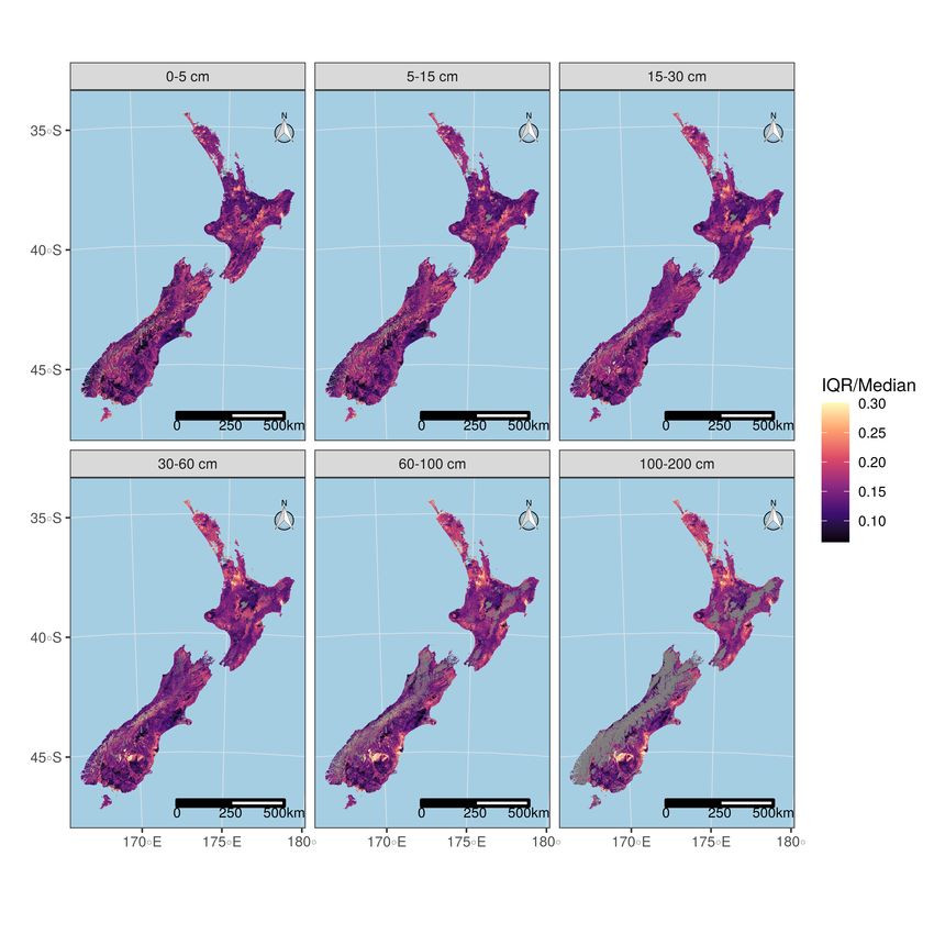
3.6. Uncertainty of the Predictions Across the Country
The uncertainties associated with the soil pH predictions were assessed using the ratio between
the inter-quartile range (IQR, i.e., the 50% prediction interval) and the median, and are mapped for each
GlobalSoilMap depth interval (Figure 9). Higher values of that ratio correspond to wider prediction
intervals (so to predictions that are more uncertain). The spatial distribution of these uncertainties is
not random across two dimensional space and depth. Overall, prediction uncertainties increase with
soil depth: this is an expected outcome, given the number of calibration points dramatically decreases
with soil depth (Table 2). These maps also outline specific areas where the model is not performing
well. For the topsoil depths (above 30 cm), the most uncertain predictions are encountered for the
peatlands in the Waikato, in hill country under native vegetation (Northland forests, Central Plateau,
Urewera and Kaimanawa ranges), and in the main mountain ranges (Ruahine, Tararua, and Southern
Alps). The prediction intervals for the semi-arid soils of Central Otago—arguably the most alkaline
soils in the country [60]—are widening very substantially for subsoil depths (below 30 cm). This is
also the case for other dry areas of the country, such as the southern East Coast of the North Island,
or South Canterbury.
Figure 9. Prediction uncertainties, represented using the IQR/Median ratio, at the different
GlobalSoilMap depth intervals. Grey areas represent parts of the landscape without soil at that depth.Remote Sens. 2020, 12, 2872 17 of 22
4. Discussion
4.1. Comparison with 2.5D DSM
The comparison between the results of our approach and of the 2.5D DSM models shows that
they both yield very similar results (Table 3). Validation R2 and CCC were slightly higher for the 2.5D
models (R2 = 0.65 vs. 0.68 and CCC = 0.79 vs. 0.8 respectively). The RMSE between both approaches
was almost identical, and much smaller than the standard deviation of the reference pH laboratory
method (RMSE = 0.54 vs. 0.53 respectively). Finally, the 2.5D models produced predictions that were
slightly more biased (bias = −0.03 vs. −0.05 for our approach), although arguably that amount of bias
could be considered negligible.
Table 3. Comparison of the performance of our approach with existing pH products (Fundamental
Soil Layers and SoilGrids) on the validation samples.
RMSE R2 CCC Bias
Our approach 0.54 0.65 0.79 −0.03
2.5D approach 0.53 0.68 0.80 −0.05
Fundamental Soil Layers 0.76 0.31 0.49 0.28
SoilGrids 250 m 0.79 0.37 0.51 0.22
To compare the uncertainties associated with both 2.5D and 3D DSM models, Nauman and
Duniway [26] introduced the Relative Prediction Interval (RPI), expressed as the ratio between the
95% prediction interval and the median of the training data. It was adapted to our study, where the
90% prediction interval was used to express model uncertainty, and calculated as the ratio between the
90% prediction interval and the median of pH in the training dataset. The statistical distribution of RPI
values calculated on the validation set for both approaches are compared in Figure 10. In contrast to
the results reported by Nauman and Duniway [26] for soil organic carbon, we did not observe higher
RPI values for our 3D approach, and overall the prediction widths for both methods were very similar.
2.5D approach our approach
2.0
Probability density
1.5
1.0
0.5
0.0
0.0 0.5 1.0
RPI
Figure 10. Comparison of the distribution of the Relative Prediction Interval (RPI) values for the 2.5D
approach and the 3D approach tested in this study.
4.2. Comparison with Other Soil pH Products for New Zealand
Validation samples were also used to assess our approach against the currently available
soil pH products for New Zealand, i.e., the Fundamental Soil Layers (FSL), a national legacy
soil information product, and SoilGrids, the main global soil information product currently
available. The results are presented in Table 3, and show that our model and the 2.5D approachRemote Sens. 2020, 12, 2872 18 of 22
significantly out-performs both existing products. The FSL and SoilGrids showed similar level of
prediction performance (R2 = 0.31 and 0.37, CCC = 0.49 and 0.51, RMSE = 0.76 and 0.79 respectively).
The scatterplots of predicted vs. observed values for our model, FSL, and SoilGrids are compared
in Figure 11, and outline in more detail the differences between the three pH products. The FSL is
a polygon-based, expert-driven soil information product, as evidenced by the binning effects in the
predicted values. Low values of pH, in particular, are poorly predicted by the FSL, possibly because
these values correspond to regions of New Zealand where expertise is less developed (i.e., soils
under native vegetation). Predictions for SoilGrids also suffer from censoring extreme values of
pH, at both ends of the spectrum (i.e., for observed pH < 4.8 or pH > 7). The predictions from the
approach used in this study produce more accurate predictions, with points closer to the grey 1:1 line.
The more acidic soils are well predicted, unlike the FSL and SoilGrids; however, as suggested by the
residuals plots (Figure 5), the alkaline soils seem to be systematically under-predicted. New Zealand
soils are generally quite acidic, a general phenomenon of southern hemisphere, temperate soils [65],
so strong model performance in the low pH range is reassuring. However, exceptional soils with
high pH, which include salt pans, some recent, sandy soils, and those derived from schist in arid
climates, can foster distinctive biological communities in New Zealand [66,67] and greater precision in
predicting these sites would be desirable for biodiversity modelling and conservation planning.
In absolute terms, the performance of our approach was satisfactory, and shows levels of
uncertainties comparable or better than published DSM-based pH maps at regional or national scale in
other parts of the world [24,26,52,68,69]. Most importantly, it represents a significant improvement on
existing soil pH maps for New Zealand.
FSL SoilGrids 250 m our approach
8
pH (observed)
6
4
4 5 6 7 8 4 5 6 7 8 4 5 6 7 8
pH (predicted)
Figure 11. Comparison of the predicted vs. observed values for the FSL and SoilGrids products, and for
the proposed approach. Results shown were calculated on the validation samples. The red line shows
the best linear fit for each model.
4.3. Limitations and Potential Improvements
The data augmentation step allowed for the inclusion of uncertainty about the soil pH
measurements: in our case, we represented this uncertainty by the standard deviation σ = 0.1,
which was derived by the laboratory using replication experiments over the recent years. There is
potential to use this mechanism to include uncertainties associated with the large range of soil
attributes measurement techniques that are now available; not only reference laboratory techniques,
but also estimates made using pedo-transfer functions, or using proximal soil sensing (such as visible
near-infrared and mid-infrared spectroscopy, portable X-ray fluorescence). In some cases, it may
require further work to derive appropriate uncertainty estimates alongside those measurements.
Furthermore, it does assume that the soil attribute value affected to the horizon is representative:
this may only be the case when sampling has been done based on pedogenetic horizons, and when the
soil property is reflected in soil morphology.Remote Sens. 2020, 12, 2872 19 of 22
There are several ways both the prediction results and the conceptual modelling framework could
be improved. Some covariates were not available for the study, but will soon be available for New
Zealand landscape, in particular a better parent material map that includes pumice and tephra deposits,
which are critical to many soil-forming processes, in particular in the North Island. Other covariates
that could potentially improve the model are related to the management effects that are affecting
soil pH distribution: better land use information could improve estimates on productive land, where
liming is practised. Similarly, the collection of more observation data to compensate for imbalance in
the calibration dataset should be aimed towards alkaline soils and non-productive land, in particular
for deeper horizons.
Other issues are inherent to the method itself: in particular, using data augmentation inflates the
number of data points to process, so computational requirements to calibrate the model are often higher
than for a 2.5D approach, unless the latter uses a very large number of horizons. The computational cost
is also very large when using the trained model to generate products, as predictions are (i) generated
for every centimetre between the soil surface and the maximum soil depth, and then (ii) an integral
is calculated from this suite of estimates to calculate values for specific depth intervals. Kriging of
residuals was not tested in this study for this reason, but should be tested in the future. Nevertheless,
we found the benefits associated with a 3D model (in particular the ability to adapt to different depth
supports depending on the stakeholder’s needs) to outweigh these issues: the use of high-performance
computing will allow to by-pass most, if not all, the computational challenges.
5. Conclusions
This study presented the first mapping of a soil attribute for New Zealand—in this instance,
soil pH—at 100 m resolution. To do so, we introduced a novel prediction method that draws virtual
samples from the actual soil observations recorded from a depth interval, which artificially augment
the training dataset. This allowed us to represent a wider range of depths associated with any given
pH measurement, but also the uncertainties associated with that measurement. The augmented dataset
was then used to train a single, 3D prediction model based on a quantile regression forest. This 3D
DSM approach to soil pH modelling had similar performance to the more established 2.5D methods,
and out-performed significantly all the existing soil pH information products currently available for
New Zealand. However, compared with the 2.5D approaches, our model was also able to cater for
the needs of a wide range of stakeholders, and we demonstrated the generation of soil pH grids for
different depth intervals.
Author Contributions: P.R. analysed the data and wrote the paper; O.R.B., S.J.R., and J.K.M. collated additional
datasets, O.R.B., S.J.R., J.K.M., A.-G.A., and G.J.G. contributed to reviewing and editing of the manuscript.
All authors have read and agreed to the published version of the manuscript.
Funding: This research was supported by Strategic Science Investment Funding for Crown Research Institutes
from the Ministry of Business, Innovation and Employment’s Science and Innovation Group.
Acknowledgments: The wetland data were sourced from the New Zealand Wetland database held by Manaaki
Whenua—Landcare Research. The authors would like to thank Anne Austin and John Drewry for their comments
on the manuscript. P.R. is member of the Research Consortium GLADSOILMAP, supported by LE STUDIUM
Loire Valley Institute for Advanced Studies.
Conflicts of Interest: The authors declare no conflict of interest.
References
1. Sparks, D.L. Environmental Soil Chemistry; Elsevier: Amsterdam, The Netherlands, 2003.
2. Neina, D. The role of soil pH in plant nutrition and soil remediation. Appl. Environ. Soil Sci. 2019, 2019, 5794869.
[CrossRef]
3. Cavanagh, J.A.E.; Yi, Z.; Gray, C.; Munir, K.; Lehto, N.; Robinson, B. Cadmium uptake by onions, lettuce and
spinach in New Zealand: Implications for management to meet regulatory limits. Sci. Total Environ. 2019,
668, 780–789. [CrossRef]Remote Sens. 2020, 12, 2872 20 of 22
4. Johnson, P.; Gerbeaux, P. Wetland Types in New Zealand; Department of Conservation: Wellington,
New Zealand, 2004.
5. Webb, T.; Wilson, A. A Manual of Land Characteristics for Evaluation of Rural Land; Landcare Research Science
Series 10; Manaaki Whenua Press: Lincoln, New Zealand, 1995.
6. Ausseil, A.G.; Lindsay Chadderton, W.; Gerbeaux, P.; Theo Stephens, R.; Leathwick, J.R. Applying systematic
conservation planning principles to palustrine and inland saline wetlands of New Zealand. Freshw. Biol.
2011, 56, 142–161. [CrossRef]
7. Ringrose-Voase, A.; Grealish, G.; Thomas, M.; Wong, M.; Glover, M.; Mercado, A.; Nilo, G.; Dowling, T.
Four Pillars of digital land resource mapping to address information and capacity shortages in developing
countries. Geoderma 2019, 352, 299–313. [CrossRef]
8. Kidd, D.; Webb, M.; Malone, B.; Minasny, B.; McBratney, A.B. Digital soil assessment of agricultural
suitability, versatility and capital in Tasmania, Australia. Geoderma Reg. 2015, 6, 7–21. [CrossRef]
9. Sparling, G.; Schipper, L. Soil quality at a national scale in New Zealand. J. Environ. Qual. 2002, 31, 1848–1857.
[CrossRef]
10. Ministry for the Environment; Statistics New Zealand. New Zealand’s Environmental Reporting Series:
Our Land 2018; Ministry for the Environment: Wellington, New Zealand; Statistics New Zealand: Wellington,
New Zealand, 2018.
11. Kidd, D.; Field, D.; McBratney, A.B.; Webb, M. A preliminary spatial quantification of the soil security
dimensions for Tasmania. Geoderma 2018, 322, 184–200. [CrossRef]
12. Landcare Research. New Zealand Fundamental Soil Layers, Soil pH. 2000. Available online: https:
//lris.scinfo.org.nz/layer/48102-fsl-ph/ (accessed on 15 July 2020).
13. Hengl, T.; de Jesus, J.M.; Heuvelink, G.B.; Gonzalez, M.R.; Kilibarda, M.; Blagotić, A.; Shangguan, W.;
Wright, M.N.; Geng, X.; Bauer-Marschallinger, B.; et al. SoilGrids250m: Global gridded soil information
based on machine learning. PLoS ONE 2017, 12, e0169748. [CrossRef]
14. Chen, S.; Mulder, V.L.; Heuvelink, G.B.; Poggio, L.; Caubet, M.; Dobarco, M.R.; Walter, C.; Arrouays, D.
Model averaging for mapping topsoil organic carbon in France. Geoderma 2020, 366, 114237. [CrossRef]
15. Arrouays, D.; Leenaars, J.G.; Richer-de Forges, A.C.; Adhikari, K.; Ballabio, C.; Greve, M.; Grundy, M.;
Guerrero, E.; Hempel, J.; Hengl, T.; et al. Soil legacy data rescue via GlobalSoilMap and other international
and national initiatives. GeoResJ 2017, 14, 1–19. [CrossRef]
16. Bishop, T.; McBratney, A.; Laslett, G. Modelling soil attribute depth functions with equal-area quadratic
smoothing splines. Geoderma 1999, 91, 27–45. [CrossRef]
17. Zhang, G.l.; Feng, L.; Song, X.D. Recent progress and future prospect of digital soil mapping: A review.
J. Integr. Agric. 2017, 16, 2871–2885. [CrossRef]
18. Jenny, H. Factors of Soil Formation: A System of Quantitative Pedology; McGraw-Hill: New York, NY, USA, 1941.
19. Minasny, B.; McBratney, A.B.; Mendonça-Santos, M.; Odeh, I.; Guyon, B. Prediction and digital mapping of
soil carbon storage in the Lower Namoi Valley. Soil Res. 2006, 44, 233–244. [CrossRef]
20. Myers, D.B.; Kitchen, N.R.; Sudduth, K.A.; Miles, R.J.; Sadler, E.J.; Grunwald, S. Peak functions for modeling
high resolution soil profile data. Geoderma 2011, 166, 74–83. [CrossRef]
21. Malone, B.P.; McBratney, A.; Minasny, B.; Laslett, G. Mapping continuous depth functions of soil carbon
storage and available water capacity. Geoderma 2009, 154, 138–152. [CrossRef]
22. Orton, T.; Pringle, M.; Bishop, T. A one-step approach for modelling and mapping soil properties based on
profile data sampled over varying depth intervals. Geoderma 2016, 262, 174–186. [CrossRef]
23. Pejović, M.; Nikolić, M.; Heuvelink, G.B.; Hengl, T.; Kilibarda, M.; Bajat, B. Sparse regression interaction
models for spatial prediction of soil properties in 3D. Comput. Geosci. 2018, 118, 1–13. [CrossRef]
24. Ramcharan, A.; Hengl, T.; Nauman, T.; Brungard, C.; Waltman, S.; Wills, S.; Thompson, J. Soil property
and class maps of the conterminous United States at 100-meter spatial resolution. Soil Sci. Soc. Am. J. 2018,
82, 186–201. [CrossRef]
25. Brus, D.; Yang, R.M.; Zhang, G.L. Three-dimensional geostatistical modeling of soil organic carbon: A case
study in the Qilian Mountains, China. Catena 2016, 141, 46–55. [CrossRef]
26. Nauman, T.W.; Duniway, M.C. Relative prediction intervals reveal larger uncertainty in 3D approaches to
predictive digital soil mapping of soil properties with legacy data. Geoderma 2019, 347, 170–184. [CrossRef]
27. Minasny, B.; McBratney, A.B. Digital soil mapping: A brief history and some lessons. Geoderma 2016,
264, 301–311. [CrossRef]You can also read