Evaluation of river flood extent simulated with multiple global hydrological models and climate forcings
←
→
Page content transcription
If your browser does not render page correctly, please read the page content below
LETTER • OPEN ACCESS

Evaluation of river flood extent simulated with multiple global
hydrological models and climate forcings
To cite this article: Benedikt Mester et al 2021 Environ. Res. Lett. 16 094010

View the article online for updates and enhancements.

                               This content was downloaded from IP address 82.83.228.19 on 24/08/2021 at 09:23
Environ. Res. Lett. 16 (2021) 094010 https://doi.org/10.1088/1748-9326/ac188d
LETTER
Evaluation of river flood extent simulated with multiple global
OPEN ACCESS
hydrological models and climate forcings
RECEIVED
17 February 2021 Benedikt Mester1,2,∗, Sven Norman Willner1, Katja Frieler1 and Jacob Schewe1
REVISED 1
16 July 2021 Potsdam Institute for Climate Impact Research, Potsdam, Germany
2
Institute of Environmental Science and Geography, Potsdam University, Potsdam, Germany
ACCEPTED FOR PUBLICATION ∗
Author to whom any correspondence should be addressed.
28 July 2021
PUBLISHED
E-mail: benedikt.mester@pik-potsdam.de
13 August 2021
Keywords: global flood model, validation, model intercomparison, flood risk, global hydrological model
Original content from
Supplementary material for this article is available online
this work may be used
under the terms of the
Creative Commons
Attribution 4.0 licence. Abstract
Any further distribution Global flood models (GFMs) are increasingly being used to estimate global-scale societal and
of this work must
maintain attribution to economic risks of river flooding. Recent validation studies have highlighted substantial differences
the author(s) and the title
of the work, journal in performance between GFMs and between validation sites. However, it has not been
citation and DOI. systematically quantified to what extent the choice of the underlying climate forcing and global
hydrological model (GHM) influence flood model performance. Here, we investigate this
sensitivity by comparing simulated flood extent to satellite imagery of past flood events, for an
ensemble of three climate reanalyses and 11 GHMs. We study eight historical flood events spread
over four continents and various climate zones. For most regions, the simulated inundation extent
is relatively insensitive to the choice of GHM. For some events, however, individual GHMs lead to
much lower agreement with observations than the others, mostly resulting from an overestimation
of inundated areas. Two of the climate forcings show very similar results, while with the third,
differences between GHMs become more pronounced. We further show that when flood
protection standards are accounted for, many models underestimate flood extent, pointing to
deficiencies in their flood frequency distribution. Our study guides future applications of these
models, and highlights regions and models where targeted improvements might yield the largest
performance gains.
1. Introduction Continental-scale changes in flood discharge have
been observed recently, in line with theoretical
Of all natural disasters worldwide, fluvial (river) expectations about the effects of global warming on
flooding is among the most frequent and devastating the hydrological cycle (IPCC 2014, Blöschl et al 2019).
hazards (Jha et al 2012). In the recent years of 2010– This poses the question to what extent the soci-
2018, it caused 115 million human displacements etal impacts of floods have already been shaped by
(IDMC 2019), 49 595 fatalities, and US$ 360 billion anthropogenic climate change. However, displace-
in economic losses (Munich Re 2020). For example, ments, damages and losses associated with floods are
11 million displacements (IDMC 2019), 1985 deaths, a function not only of the physical flood hazard, but
and US$ 9.5 billion in economic losses (EM-DAT also of socioeconomic factors. The latter, in partic-
2020) were recorded in the aftermath of the Pakistan ular, determine exposure—the number of people or
floods in 2010. Flooding killed 6054 people in India in the value of assets potentially affected by flooding—,
2013 (EM-DAT 2020) and caused an estimated US$ and vulnerability—the susceptibility of exposed ele-
33 billion losses in China in 2016, with only 2% of ments to the hazard (IPCC 2012, Jongman et al
losses insured (Floodlist 2016). Beyond these records, 2015). Together, these controlling risk factors form
one can expect further losses such as of cultural her- a dynamic, spatially and temporally variable balance
itage and ecosystem services, which are, however, dif- used for risk assessment. Since not all three factors
ficult to assess (Hurlbert 2018). are generally known, it is challenging to quantify their
© 2021 The Author(s). Published by IOP Publishing Ltd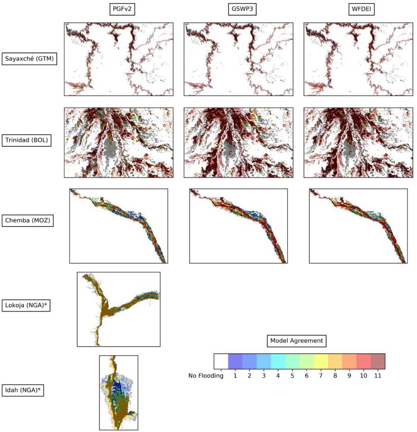
Environ. Res. Lett. 16 (2021) 094010                                                                     B Mester et al

relative contributions to the ultimate impacts of his-      simulation ensemble against satellite-derived flood
torical floods.                                             extent observations for eight recent large flood events
     Global flood models (GFMs) can be used to              on four continents, covering different climatic and
estimate historical flood extents based on observed         hydraulic environments, and assess the influence of
weather, and could thereby provide the physical flood       the choice of both climate forcing and GHM on the
hazard component for such assessments when dir-             performance of the GFM simulations. We do this
ect observations of flood extent are lacking. This          under different assumptions about flood protection,
approach is increasingly being used, for instance, to       to also assess the realism of simulated return intervals.
estimate past changes in vulnerability (Tanoue et al
2016) or attribute trends in reported flood-induced         2. Data and methodology
damages (Sauer et al 2021). However, the degree to
which such studies can explain the observed vari-           2.1. Models
ations in damages and affected population varies sub-       We use the GFM CaMa-Flood (Yamazaki et al 2011),
stantially, and can be fairly low for many parts of the     driven by an ensemble of 11 GHMs and three grid-
world. It is unclear to what extent this is due to short-   ded climate forcing datasets, leading to 33 combin-
comings in the simulated flood hazard, exposure, or         ations in total. The climate forcing datasets used to
assumptions about vulnerability.                            drive the GHMs are the Princeton Global Forcing
     This highlights that a thorough understanding          data set version 2 (PGFv2) (Sheffield et al 2006), the
of the reliability of global flood hazard estimates is      Global Soil Wetness Project phase 3 forcing data set
important. However, validation and benchmarking             (GSWP3) (Hyungjun 2014) and the WATCH forcing
studies are rare (Hoch and Trigg 2019), which is            data methodology applied to ERA-Interim reana-
mainly due to the scarce availability of reference flood    lysis data (WFDEI) (Weedon et al 2011, 2014). All
maps outside of some high-income countries and              three datasets are based on reanalysis products (ERA-
regions such as the European Union, North Amer-             Interim for WFDEI; 20CR for GSWP3; NCEP/N-
ica, or Australia (Dottori et al 2016). A compar-           CAR for PGFv2) that assimilate information from
ison of several GFMs to satellite imagery in three          local weather stations, and subsequently apply cor-
African river sections showed considerable differ-          rections to the precipitation data and other variables
ences between models in terms of how accurately they        using station-based observational data; two datasets
reproduced observed flood extent; most models both          (WFDEI and GSWP3) also correct for precipita-
missed flooding in some areas and falsely simulated         tion undercatch by rain gauges. Given these meth-
flooding in others (Bernhofen et al 2018). The agree-       odologies, and the gridded nature of the forcing
ment between these models in simulated flood extent         products, direct comparison with local station data is
was shown to be only 30%–40%, with considerable             not straightforward, but existing validation exercises
differences in hazard magnitude and spatial patterns        show reasonable agreement with station data as well
(Trigg et al 2016).                                         as with gridded observational datasets (Weedon et al
     It is hardly known to what extent such differences     2014, Essou et al 2017).
between GFM simulations and their predictive capa-               The set of GHMs comprises CLM4.0 (Leng et al
cities are related to the GFMs themselves, for instance,    2015), DBH (Tang et al 2007), H08 (Hanasaki et al
due to differences in model structure or the underly-       2008), JULES-W1 (Best et al 2011), LPJmL (Sitch
ing digital elevation models; and to what extent they       et al 2003), MATSIRO (Pokhrel et al 2014), MPI-HM
are related to the boundary conditions used to force        (Stacke and Hagemann 2012), ORCHIDEE (Traore
the GFMs. Depending on the modelling framework,             et al 2014), PCR-GLOBWB (Wada et al 2014), VIC
these boundary conditions consist either of gauged          (Liang et al 1994) and WaterGAP2 (Müller Schmied
river flow datasets, or—for the majority of GFMs—           et al 2016). An overview of the GHMs’ main char-
of gridded runoff estimates from global hydrological        acteristics, e.g. evaporation and runoff schemes, is
model (GHM) or land-surface models (Trigg et al             available in the supplementary material—table S1.
2016). Those runoff simulations in turn need meteor-        All GHM simulations follow a common protocol
ological variables as input, which come from global         (ISIMIP2a, www.isimip.org) to ensure a standard-
climate reanalyses or climate models. Most global           ized input scheme for CaMa-Flood. Simulations are
flood hazard simulations thus are the result of a cas-      performed under naturalized conditions, i.e. storage
cade of different models and data products, with mul-       in man-made reservoirs or agricultural water with-
tiple options available at each step in the cascade. The    drawal are not included.
influence of choices in the upstream steps of this cas-          The runoff of the respective GHM then consti-
cade on the resulting flood extent estimate has hardly      tutes the input for CaMa-Flood v3.6.2 which yields
been systematically investigated (Zhou et al 2021).         discharge as well as flood depth on a 0.25◦ resolution
     In this study we address this research gap. We run     grid. The underlying river network in CaMa-Flood
a state-of-the-art GFM with runoff forcing from 11          has been derived by the model author based on the
different GHMs, each in turn forced by three dif-           flow direction maps HydroSHEDS (Lehner et al 2008)
ferent climate reanalyses. We evaluate the resulting        and GDBD (Masutomi et al 2009) as well as the digital

                                               2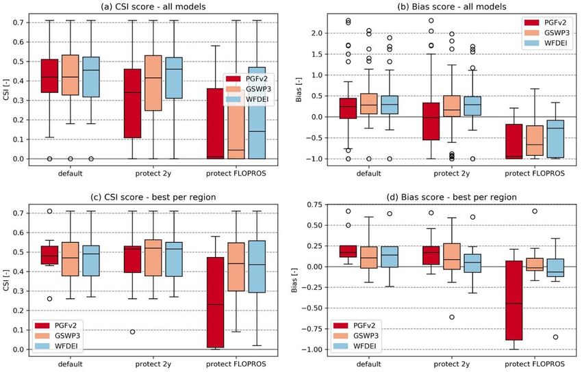
Environ. Res. Lett. 16 (2021) 094010 B Mester et al
elevation model SRTM3 (Farr et al 2007) using their models evaluated here are likely inferior to more
FLOW method (Yamazaki et al 2009). Using these complex, locally-informed flood prediction mod-
same data, we downscale flood depth to 18 arc sec. els where those exist, the global models nonetheless
i.e. the daily flood volume in a low-resolution (0.25◦ ) are important tools widely used in continental- or
grid cell is distributed onto the underlying high- global-scale applications (Bates et al 2021).
resolution (18 arc sec) grid cells according to their
elevation. We then assign to each high-resolution grid 2.2. Observational data
cell the annual maximum daily value, resulting in an For the comparison of our simulated flood extent
annual flood depth timeseries. The event duration we use satellite imagery from the archive of the
according to the satellite imagery matches with the Dartmouth Flood Observatory (DFO), which is
rising limb or the peak of the flood simulations for based on NASA MODIS satellite sensors (https://
most regions of interest; and coincides with no second floodobservatory.colorado.edu/) (Brakenridge 2006),
flood event in the year of investigation, which legit- and from the UNOSAT Flood Portal (UFP) providing
imizes this approach (figures S22–S33 in the supple- flood extent maps derived from a variety of satellite
mentary material (available online at stacks.iop.org/ sensors (http://floods.unosat.org/geoportal/catalog/
ERL/16/094010/mmedia)). This dataset is used to main/home.page). The number of eligible events is
produce figure 2. Finally, we calculate the flooded limited, because consistent geospatial imagery starts
fraction on an intermediate-resolution (2.5 arc min) in 2010 for DFO and 2006 for UFP, respectively,
grid, i.e. the fraction of flooded high-resolution grid and most the climate reanalysis products used here
cells within each intermediate-resolution grid cell. extend only until 2010 or (for PGFv2) 2012. Only
This flood fraction dataset is used to calculate the per- large-scale disasters with a large river size are taken
formance scores (see below). into account to ensure that the inundated areas can
Whereas this constitutes our default simulation be adequately captured given the spatial resolution
setup (‘default’), we also assess setups assuming pro- of the GFM. It is essential that observational valida-
tection against floods with an average recurrence tion data is available, consistent and comprehensive
interval (ARI) of 2 years (‘protect 2y’ setup), and for the entire area of interest. Additionally, a spread
assuming flood protection standards according to the across different climate zones and continents is desir-
FLOPROS database (Scussolini et al 2016) (‘protect able for a comprehensive global comparison study
FLOPROS’ setup). FLOPROS incorporates modelled (Dottori et al 2016). We exclude flash flood events,
protection, infrastructure, and policy measures in a storm surge flooding, as well as floods caused by
best estimate (‘merged’ layer) on a sub-national level. mismanagement or failure of man-made structures,
Fitting, for each climate forcing and GHM, a general- since these types of floods cannot be modelled by the
ized extreme value (GEV) distribution to the annual GFM.
maximum discharge for each cell and in the simu- We identify ten regions of particular interest in
lation period available for all models (1971–2010), the context of eight major flood events, as shown
we obtain the return period in dependence of dis- in figure 1. The following regions, named after the
charge. We then compare the return period for each central city or town affected, are used for valida-
studied event to the protection level for the respective tion: Huainan in China (year of flood event: 2007),
cell; i.e. either 2 years, or the protection level given by Sayaxché in Guatemala (2008; the westernmost part
FLOPROS. In the ‘protect’ settings, we thereby only is located in Mexico), Trinidad in Bolivia (2008),
account for flood events in cells in which this pro- Alipur and Ghotki in Pakistan (2010), Phimai in
tection level is exceeded and assume no flooding for Thailand (2010), Dalby in Australia (2010), Chemba
events with lower return period. in Mozambique (2007), as well as Lokoja and Idah
It should be noted that there are well-established in Nigeria (2012). Chemba (MOZ; we will indicate
practices used in floodplain planning processes each location’s ISO3 country code throughout the
internationally (World Meteorological Organization paper for ease of reference), Lokoja (NGA), and Idah
2009) that do not rely on GFMs but instead use more (NGA) are studied in a recent GFM intercompar-
complex, locally calibrated hydrodynamic models ison study, thus facilitating comparison of our results
(Raadgever and Hegger 2018). However, these tech- with that study (Bernhofen et al 2018). The selected
niques require elaborate calibration for each indi- areas are located in monsoon climates, tropical savan-
vidual catchment (Canning and Walton 2014), and nas and rainforests, subtropical climates, and deserts,
rely on local observational data that is not commonly on four continents (Peel et al 2007). The selection
available in all parts of the world. For instance, in covers a variety of hydraulic characteristics, ranging
a new, comprehensive global streamflow database from confined watercourses of the Niger River and
(Do et al 2018, Gudmundsson et al 2018), local the anabranching Condamine River in Queensland to
gauge records are available for only one of the events highly braided and slow sections of the Indus River.
studied in this paper (the 2010 flood in Dalby, Aus- A more detailed description of the chosen events and
tralia; see below), and are entirely unavailable for the river hydraulics can be found in the supplement-
some of the study regions. Thus, while the global ary material—table S2.
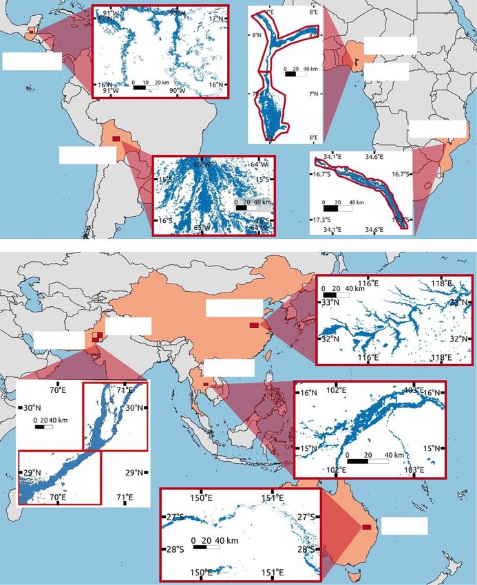
3Environ. Res. Lett. 16 (2021) 094010 B Mester et al
Figure 1. Satellite imagery of flood extent (blue) in the study areas (red). Note: the outlines of Chemba (MOZ), Lokoja (NGA)
and Idah (NGA) follow the flood shape and are not rectangular. Country shapes reproduced from https://gadm.org/data.html.
The satellite imagery of flood extents for the (NGA) are derived from Research Data Leeds (http://
regions Alipur (PAK), Ghotki (PAK), Phimai (THA), archive.researchdata.leeds.acuk/411/), which is inten-
and Dalby (AUS) are taken from the DFO. Satel- ded for GFM validation (Bernhofen et al 2018) and
lite imagery for Huainan (CHN), Sayaxché (GTM) also based on the DFO archive. In contrast to the
and Trinidad (BOL) are downloaded from the UFP. other regions, data for these regions is only available
For some events, the data consists of several days inside an irregularly shaped polygon roughly out-
of imagery and is hence merged into one maximum lining the main inundation area, which limits the ana-
flood extent per event. Rectangular analysis regions lysis of both observations and simulations to these
are defined for the events above (red rectangles in polygons (we will discuss the implications of this
figure 1). Flood footprints and outline data for the below). The satellite imagery for all regions is at
regions Chemba (MOZ), Lokoja (NGA) and Idah a 209 m resolution. Only the simulations of eight
4Environ. Res. Lett. 16 (2021) 094010 B Mester et al
GHMs forced with PGFv2 extend to the year 2012, we thus compute absolute flooded area per cell for
which limits the analysis of Lokoja (NGA) and Idah both CaMa-Flood output and satellite imagery. Sum-
(NGA). ming over all cells within an analysis region yields F m
and F o respectively. The intersection area F m ∩ F o is
2.3. Analysis calculated analogously but multiplying, in each cell,
The analysis procedure starts with a visual compar- the smaller flooded fraction of either CaMa-Flood or
ison of the simulated and the observed flood extent. satellite data with the cell area; for the union area
For the former, we use the gridded CaMa-Flood flood F m ∪ F o the larger value of either model or data is
depth output downscaled to 18 arc sec resolution used. This approach is based on the assumption that
(approx. 550 m at the equator). This yields a binary the location of flooding at the sub-grid scale is, for
grid with two grid cell states (flooded or not flooded) a given grid-scale flood extent, constrained by topo-
for each climate forcing and GHM. For each climate graphy. For comparison, we also show CSI and Bias
forcing and grid cell we then count the number of scores computed directly on 18 arc sec resolution in
GHMs showing flooding in the respective cell, to cre- supplementary material figures S36 and S37.
ate a model agreement map. We use the flood outlines In the section 3, along with the performance
for each region (red outlines in figure 1) to mask both metrics for individual simulations and regions, we
the model agreement map and the satellite imagery. also show the median over all regions as well as
The masked images are then superimposed onto each median, minimum, maximum and spread over all
other (figure 2). Next, in order to quantify model per- hydrological models. Lokoja (NGA) and Idah (NGA)
formance, we use two different performance metrics were excluded from the computation of the regional
(Bates and de Roo 2000, Aronica et al 2002, Werner median, in order to allow a fair comparison of the
et al 2005, Bernhofen et al 2018). First, the critical suc- median values between the three climate forcing
cess index (CSI) is defined as: datasets.
Fm ∩ Fo 3. Results
CSI =
Fm ∪ Fo
We first analyse results for the default simulations not
where F m is the modelled flooded area by CaMa-
accounting for flood protection; and subsequently,
Flood and F o is the observed flooded area by the satel-
in section 3.3, discuss the simulations with flood
lite imagery. F m ∩ F o is the intersection area between
protection.
modelled and observed flood extent, i.e. the area cor-
rectly simulated as flooded by the model; and F m ∪ F o
3.1. Model agreement map
is the union area between modelled and observed
Figure 2 displays the model agreement overview
flooded area. The CSI is perceived as the one of the
for all three climate forcings and ten regions, for
most comprehensive scores (Bernhofen et al 2018). It
the default simulations. Results differ substantially
ranges from 0 to 1, where 1 represents a perfect model
between the regions. The agreement between mod-
‘fit’ (Sampson et al 2015), and penalizes overpredic-
els is high, and the simulated flood outline in relat-
tion. The Bias score is defined as:
ively good agreement with observations, for Sayaxché
(Fm ∩ Fo ) + Fm (GTM), Trinidad (BOL), Lokoja (NGA), Idah (NGA),
Bias = − 1. and Phimai (THA), although the models miss some
(Fm ∩ Fo ) + Fo
extended parts of the flood in Trinidad (BOL) and
An unbiased model has a Bias score of 0, positive and Phimai (THA), and somewhat overestimate the flood
negative values indicate a tendency towards over- or extent in Idah (NGA). Agreement between models is
under prediction of flood extents, respectively. The also high (indicated by reddish colours) in Huainan
Bias score rewards a large intersection area between (CHN); however, the models overestimate the extent
modelled and observed flood extent. of flooding there, including a large area in the north-
At high spatial resolution, mismatches in river western part of the region where most models falsely
geometry between the satellite imagery and the digital simulate flooding. In Chemba (MOZ), as well as
elevation models used in the GFM could deteriorate in Alipur (PAK) and Ghotki (PAK), most models
the performance scores in confined floodplains; e.g. agree on flooding along the main river branches, but
if a river channel in the DEM is offset relative to its partly underestimate the extent of this flooding; while
real location (Yamazaki et al 2011). Since we want to many models falsely simulate flooding in an extensive
evaluate simulated flood extent per event, rather than area to the east of the Indus River in Ghotki (PAK),
DEM accuracy, we therefore calculate performance and along the Sutlej river estuary in Alipur (PAK).
scores at the coarser resolution of 2.5 arc min. For Finally, in Dalby (AUS), only some models capture
that, we downsample both the binary satellite imagery the more extensive parts of the flood; at the same
and the CaMa-Flood binary flood data to 2.5 arc min time, several models simulate flooding alongside long
using simple linear sampling, yielding the share of stretches of the river channel where no flooding is
flooded area per cell. Incorporating absolute cell area observed.
5Environ. Res. Lett. 16 (2021) 094010 B Mester et al
Figure 2. Model agreement map indicating the flood extent overlap between the 11 GHMs and the satellite data for each study
region (row) and climate forcing (column). The cell colour represents the number of GHMs that computed the corresponding
cell to be flooded. The underlying flood extent of the satellite imagery (light grey) is assigned a dark colour tone if it matches with
at least one GHM. For the 2012 flood in Lokoja (NGA) and Idah (NGA) (marked with an asterisk ∗ ), only eight GHMs, driven
with PGFv2, were available.
6Environ. Res. Lett. 16 (2021) 094010 B Mester et al
Figure 2. (Continued.)
The simulation of flooding in large areas where and Huainan (CHN), with most or all GHMs. This
no flooding was observed—found for the floods in partly remedies the overestimation of flooding out-
China, Pakistan, and Australia—could theoretically side the main river floodplains, but also leads to
be induced by contamination of our flood extent a more substantial underestimation of flood extent
estimate by a different flood event: i.e. an event occur- along the main rivers in Alipur (PAK) and Ghotki
ring in the same year which had an even higher flood (PAK), compared to the other two forcing datasets.
magnitude in that part of the region, and would thus
be picked up when taking the annual maximum dis- 3.2. Model performance scores
charge in every grid cell. However, analysis of daily In line with the observations from the model agree-
flood data confirms that this is not the case; while ment maps, the CSI scores vary substantially between
there can be a considerable delay of the flood peak the different regions (figure 3). A comparatively
in CaMa-Flood compared to observations (Zhao et al low CSI is found for Alipur (PAK), Ghotki (PAK),
2017), the estimated flood extent is largely related Huainan (CHN), with scores between 0.3 and 0.4, and
to one coherent flood event, except for outliers in especially Dalby (AUS) with scores below 0.3. High
marginal grid cells (supplementary material, figures CSI scores of around 0.5 and higher are found for
S1–S33). Sayaxché (GTM), Trinidad (BOL), Chemba (MOZ),
Regarding the climate forcing, the GSWP3 and Lokoja (NGA), and Idah (NGA). Intermediate scores
WFDEI reanalysis datasets lead to very similar results. of around 0.45 are found for Phimai (THA). Since
The PGFv2 dataset leads to markedly smaller simu- the CSI score also depends on the flood magnitude
lated flood extents in Alipur (PAK), Ghotki (PAK), (Stephens et al 2014), this numerical comparison
7Environ. Res. Lett. 16 (2021) 094010 B Mester et al
Figure 3. CSI scores for all combinations of GHMs and PGFv2 (top), GSWP3 (middle), and WFDEI (bottom) forcing. The
‘Median Region’ across the even number of regions is calculated as the mean of the two middle values. Lokoja (NGA) and Idah
(NGA) (marked with ∗ ) were excluded from the computation of the ‘Median Region’. ‘-’ means no input data was available and a
black box indicates the best-performing GHM(s) for a given region.
between regions and events should be interpreted in figure 3) is by far largest for Chemba (MOZ). This
with caution, and in conjunction with the model is primarily because there the CSI with the VIC model
agreement maps. In particular, for a given region with is zero for all three forcings, and the CSI with the
a concave topography (e.g. extensive floodplain), the MATSIRO model is zero for the PGFv2 forcing; indic-
larger the flood magnitude, the more the flood extent ating that there is no intersection between simulated
will be constrained by topography, and the less vari- and observed flood extent. The MATSIRO model
ation in flood extent will be induced by a given vari- with PGFv2 forcing also has very low CSI scores in
ation in flood discharge; potentially leading to more Alipur (PAK) and Ghotki (PAK). However, even if the
favourable CSI scores than for smaller floods. These MATSIRO and VIC models were excluded, Chemba
caveats however do not affect comparison between (MOZ), Alipur (PAK) and Ghotki (PAK) would still
models and datasets within one region and event, remain the regions with the largest differences in
which we turn to next. CSI scores across GHMs, under the PGFv2 forcing;
We find differences in performance between cli- for instance, compare CLM and PCR-GLOBWB for
mate forcings and between GHMs to be mutually Alipur (PAK) and Ghotki (PAK), or MPI-HM and
dependent, and we discuss them together in the fol- ORCHIDEE for Chemba (MOZ). Using the other
lowing. The spread across GHMs (rightmost column two climate forcings, these inter-GHM differences are
8Environ. Res. Lett. 16 (2021) 094010 B Mester et al
Figure 4. CSI scores for all combinations of GHMs and WFDEI for ‘protect 2y’ (top) and ‘protect FLOPROS’ (bottom).
The ‘Median Region’ across the even number of regions is calculated as the mean of the two middle values. Lokoja (NGA) and
Idah (NGA) were excluded from the computation of the ‘Median Region’. A black box indicates the best-performing GHM(s) for
a given region.
much smaller, mostly with a difference of about 0.1 or hand, in Huainan (CHN), all GHMs achieve substan-
less between the scores of the best and worst perform- tially higher scores with PGFv2 than with GSWP3 or
ing model. WFDEI.
The median CSI scores over all regions (bottom There is thus no climate forcing dataset that per-
row in each subplot in figure 3) indicate that none of forms best in all regions; nor is there one GHM which
the GHMs performs consistently better or worse than consistently performs best in all regions and with all
the others. Even the VIC model, which fails to cap- forcings (see black boxes in figure 3).
ture the flood in Chemba (MOZ), achieves reasonable We now turn to the Bias scores. While a low
scores in the other regions, and has a region-median CSI score generally already implies a high bias,
CSI only slightly below the other GHMs (between the Bias score additionally indicates whether the
0.36 and 0.39 depending on the climate forcing). The observed total flood extent is over- or under pre-
MATSIRO model, which shows very low CSI scores in dicted by the model. We find that with WFDEI
three of the regions under PGFv2 forcing, is among and GSWP3 forcing, Bias scores are generally either
the best performing GHMs in some of the other small or positive (with the exception of VIC in
regions; in particular, it achieves the highest CSI score Chemba (MOZ)) (figure 4). This confirms the obser-
of all GHMs in Huainan (CHN) for all three forcings, vation made in the model agreement maps that flood
and has the highest region-median CSI score under extent is generally either matched relatively well, or
the WFDEI forcing. overestimated, by the model simulations. With the
Similarly, the statistics over all GHMs (rightmost PGFv2 climate forcing, the overall result is similar,
four columns in figure 3), and the combined statistics but substantial negative Bias scores—indicating an
across regions and GHMs (bottom right in each sub- under prediction of flood extent—occur in several
plot in figure 3, as well as figure 5), show that neither cases: for Alipur (PAK), Ghotki (PAK), and Chemba
of the three climate forcing datasets is generally super- (MOZ), with CLM, MATSIRO, and MPI-HM; cor-
ior to the others: the GHM-region median CSI is 0.42, responding to the anomalous CSI values for these
0.43, and 0.44, respectively, for PGFv2, GSWP3, and combinations described above. On the other hand,
WFDEI. PGFv2 exhibits slightly lower GHM-median the PGFv2 forcing leads to much smaller (posit-
CSI scores, and lower minimum scores, than the other ive) biases than the other two forcings in Huainan
two forcings in many of the regions; on the other (CHN).
9Environ. Res. Lett. 16 (2021) 094010 B Mester et al
Figure 5. Comparison of CSI and Bias scores between the default setting (‘default’), protection against floods with an ARI of
2 years (‘protect 2y’) and protection standards according to FLOPROS (‘protect FLOPROS’) for the climate forcings PGFv2,
GSWP3 and WFDEI. Figures (a) and (b) include all GHMs and regions, (c) and (d) only account for the best GHM per region.
The regions Lokoja (NGA) and Idah (NGA) were excluded from the computation.
Calculating the performance scores on the higher- among models and among forcings increases not-
resolution (18 arc sec) binary flood outputs confirms ably compared to the default simulations (figures 5(a)
these overall results, though the scores are somewhat and (c)).
lower (supplementary material, figures S36 and S37). This pattern becomes even more pronounced
when assuming flood protection according to FLO-
3.3. Flood protection PROS. CSI scores degrade in the majority of regions
We now analyse the simulations accounting for flood and forcing-GHM combinations (figures 4, 5 and
protection infrastructure, by counting only those supplementary figure S41). While all of the ‘pro-
flooded pixels whose ARI (estimated through fitting tect FLOPROS’ simulations still exhibit significant
a GEV function) is longer than either 2 years (‘protect CSI scores in Trinidad (BOL), they all show zero
2y’) or the protection standard indicated in the global or almost zero CSI in Dalby (AUS). In most other
database FLOPROS (Scussolini et al 2016) (‘protect regions, we find both: multiple GHM-forcing com-
FLOPROS’). binations that still achieve relatively high CSI scores,
Under the WFDEI forcing, CSI scores in the ‘pro- often preserving the maximum CSI for the region
tect 2y’ simulations change only little compared to the found in the ‘default’ setup; as well as many combin-
default simulations. Most notably, there are now two ations showing zero or very low CSI scores. Chemba
GHMs simulating no flooding in Chemba (MOZ): (MOZ) is an interesting case as here the CSI score
WaterGAP2, in addition to VIC; and the CLM model drops to zero for most of the ‘protect FLOPROS’
shows lower CSI scores in Alipur (PAK) and Dalby simulations, while, with WFDEI forcing, one single
(AUS) (figure 4). More widespread deterioration of GHM (PCR-GLOBWB) still achieves the same CSI as
CSI scores appears under the other two forcings. With in the default setup; and the same is true for three
GSWP3, there are multiple GHMs each in Chemba GHMs (CLM, ORCHIDEE, and PCR-GLOBWB)
(MOZ), Alipur and Ghotki (PAK) that show no or with GSWP3 forcing.
almost no flooding (supplementary figure S39). With While the Bias scores were mostly positive in the
PGFv2, the CSI drops to zero in Chemba (MOZ) ‘default’ simulations, the ‘protect FLOPROS’ setup
for almost all models, with the exception of DBH mostly results in negative biases, which are in many
which still shows a high CSI score there; and CSI parts of substantial magnitude (figures 5(b) and
scores in Huainan (CHN) are seriously degraded for supplementary figure S42). This corresponds to the
all GHMs. In summary, while for most regions the decreased and, often, zero CSI scores found in this
maximum CSI scores achieved are preserved when setup. Bias scores in the ‘protect 2y’ setup are, as
assuming protection against ARI of 2 years, the spread expected, closer to those in the ‘default’ setup; with
10Environ. Res. Lett. 16 (2021) 094010 B Mester et al
more pronounced overestimation of flood extent that both the overall match between models and
under WFDEI forcing, and more pronounced under- observations, and the level of agreement among
estimation in some regions under PGFv2 forcing models, differ depending on the region and event
(supplementary figure S40). that is analysed. This may be explained by varying
Considering the entire simulation ensemble, the topographies among the regions, leading to differ-
lowest median bias in flood extent is achieved in the ent errors in simulated flood extent due to cross-
‘protect 2y’ setup, in particular the simulations forced floodplain slopes. Another important caveat is that
with PGFv2 and GSWP3 yielding a lower median the shape of the study area is not consistent across
bias than in the ‘default’ setup (figure 5(b)). On regions. While the study areas for most regions are
other hand, the spread among simulations is largest rectangular and include large parts where no flood-
for ‘protect 2y’. In the ‘protect FLOPROS’ setup, the ing was observed, the study areas for Chemba (MOZ),
majority of simulations show a large negative bias, Lokoja (NGA), and Idah (NGA) are irregularly
as discussed above. However, when considering for shaped polygons narrowly outlining the observed
each region only the best-performing model, the flood extent along the main river channels. This
least biased results are achieved with WFDEI forcing means that potential flooding along tributaries is
in the ‘protect FLOPROS’ setup; the corresponding excluded from the analysis (supplementary figures
GSWP3 simulations being only slightly more biased S45–S48). Considering an example of a model over-
(figure 5(d)). estimating observed flood extent, the overestimation
may appear less severe if parts of the flood that are fur-
4. Discussion and conclusions ther away from the main channel are cut off. With the
rectangular study areas, such excess simulated flood
A number of key results emerge from our analysis: extent would be more visible and would degrade the
CSI score to a larger degree. This might go some way
(1) The performance of a global river flood model- in explaining why Chemba (MOZ), and especially
ling chain in reproducing observed flood extent Lokoja (NGA) and Idah (NGA), exhibit systematic-
for major recent floods differs considerably ally higher CSI scores than other regions. These scores
between events. While CSI scores of 0.7 and are similar to those found for the same three regions
higher are obtained for Chemba (MOZ), Idah by Bernhofen et al (2018), who used the same study
(NGA), Lokoja (NGA) (similar as in Bernhofen area outlines. This may indicate that the general level
et al (2018)), scores are much lower for many of model performance found in our study is compar-
other events, dropping below 0.3 for Dalby able to that in Bernhofen et al (2018), and that the
(AUS). lower CSI scores in the additional regions in our study
(2) The choice of GHM and climate forcing have may also be related to the layout of the study area,
mutually dependent effects on flood model per- rather than only to a poorer model performance in
formance. those regions.
(3) PGFv2 performs somewhat poorer than the Regarding key result no. 2, the importance of the
other two climate forcing datasets for many choice of GHM is confirmed by a recent study that
regions and GHMs, but better for some. The per- compared different sources of uncertainty in CaMa-
formance spread between GHMs is largest with Flood estimates: the GHM runoff inputs, variables
PGFv2. for flood frequency analysis and fitting distributions
(4) No climate forcing or GHM performs best for (Zhou et al 2021). Of these three, the GHMs were
all regions. Considering the median over all found to be by far the largest source of variation in the
regions, the PCR-GLOBWB model stands out as estimate of flood depth and inundation. That study
achieving the best, or among the best, results used a single reanalysis forcing dataset (WFDEI) as
for all forcings and in particular for the ‘protect’ input to the GHMs and did not evaluate different
setups. GHMs’ performance in relation to observed flood-
(5) Accounting for flood protection according to ing; rendering our study a useful complement. It
the FLOPROS database dramatically degrades should be pointed out that the hydrological mod-
the average agreement between simulations and elling approach underlying many of these GHMs is
observations, by reducing or eliminating simu- traditionally aimed at evaluating water and energy
lated flood extent in many cases. However, indi- balances at longer timescales (also termed catchment
vidual forcing-GHM combinations remain in yield-type models, in contrast to rainfall-runoff-type
almost every region that achieve high CSI and models), without specific focus on flood generation;
low Bias scores. which may partly explain their deficiencies in estimat-
ing flood magnitudes and timing. Disparities between
Regarding key result no. 1, we reiterate that CSI GHM-simulated and actual runoff may thus be a fun-
scores should not be compared between regions at damental reason for the relatively poor performance
face value, because of the varying flood extents. of the flood modelling methodology applied here,
However, it is also evident from the maps in figure 2 compared to conventional basin-scale flood analysis;
11Environ. Res. Lett. 16 (2021) 094010 B Mester et al
also affecting the results summarized in key results remembered that the FLOPROS protection levels are
no. 3 and 4. purely model-based estimates for most of the events;
Regarding key result no. 3, Müller Schmied et al except for those in Mozambique, China and Australia,
(2016) evaluated hydrological simulations with a where information about the actual design standards
single GHM (WaterGAP2) driven by the same cli- or about corresponding policy regulations entered
mate forcing datasets as in our study, and found the estimates provided in the database. Thus, FLO-
substantial differences in long-term average runoff PROS values may not exactly reflect the flood pro-
and other hydrological indicators. In particular, rel- tection standards actually implemented in the study
atively low precipitation and runoff estimates were regions.
found with PGFv2, compared to GSWP3 and WFDEI; Reported estimates of the average recurrence
likely related to the lack of a precipitation under- interval (ARI) are only available for some of the flood
catch correction in this dataset, but potentially also events studied here, and available estimates often dif-
to a different observational product that precipita- fer between sources and/or come with considerable
tion was corrected against (CRU TS3.21 for PGFv2; uncertainties. Nevertheless, the actual ARI appears to
GPCC version 6 for GSWP3 and WFDEI). While run- be higher than the FLOPROS protection standard for
off extremes were not directly assessed in that study, most events (supplementary table S3). This suggests
systematically lower precipitation forcing could non- that the deterioration of model results when apply-
etheless explain the larger negative biases in flood ing FLOPROS may not be predominantly related to
extent that we find in our default simulations with errors in FLOPROS. Instead, it suggests that the ARI
PGFv2 for some regions and GHMs; and might like- in the affected model simulations may be too short;
wise explain the smaller positive biases and higher i.e. the model too frequently simulates a flood of the
CSI scores in Huainan (CHN), where flood extent given magnitude.
is strongly overestimated with GSWP3 and WFDEI The ‘protect FLOPROS’ simulations thus serve to
forcing. highlight those GHM-climate forcing combinations
Nevertheless, the differences even between that correctly simulate an ARI larger than the protec-
GSWP3- and WFDEI-driven flood simulations high- tion standard, according to FLOPROS. For instance,
light some remaining uncertainty in the forcing data. applying FLOPROS, the CSI for Chemba (MOZ)
To test whether using observational datasets directly drops to zero for almost all simulations except for
as input to the GHMs might be beneficial, we per- PCR-GLOBWB with GSWP3 and WFDEI forcing,
formed a set of simulations where, for each event and for CLM and ORCHIDEE with GSWP3 for-
and grid cell, the return period simulated by a given cing (supplementary figure S41). Similarly, impos-
GHM-forcing combination was mapped to the cor- ing FLOPROS flood protection levels in Sayaxché
responding flood volume given by a benchmark sim- (GTM), the majority of models still achieve a reas-
ulation of MATSIRO which was driven with station- onable CSI with GSWP3 and WFDEI forcing but
based (GPCC) rather than reanalysis precipitation simulate no flooding with PGFv2 forcing. In Alipur
data (Kim et al 2009). This adjustment procedure (PAK) and Ghotki (PAK), only JULES-W1 and PCR-
was originally devised to correct biases in climate GLOBWB realistically simulate a large ARI with all
model-derived runoff (Hirabayashi et al 2013), and three climate forcings. Interestingly, not a single sim-
has been applied in other global flood modelling ulation shows substantial flooding in Dalby (AUS) in
studies (Dottori et al 2018, Willner et al 2018, Sauer the ‘protect FLOPROS’ setup; suggesting that here,
et al 2021). However, in our study, the adjustment the protection standard of a 100 year ARI assumed
using the MATSIRO benchmark simulation does not in FLOPROS may indeed be too high; which is also in
systematically improve the agreement between sim- line with reports of a 90 year ARI for the 2010/2011
ulated and observed flood extent (supplementary flood event (supplementary table S3).
material figures S43 and S44); suggesting that neither Generally though, many of the runoff simulations
a particular GHM nor the observations-based pre- used here may still be in need of improvement with
cipitation forcing are generally superior to the GHM respect to the high-end of the runoff distribution.
ensemble and the reanalysis-based forcings studied Indeed, a recent evaluation of monthly runoff sim-
here, respectively. ulated by six GHMs, including H08, LPJmL, MAT-
Regarding key result no. 5, one striking finding SIRO, PCR-GLOBWB, and WaterGAP2, found that
is that the incorporation of flood protection stand- most models—except MATSIRO and WaterGAP2—
ards according to FLOPROS leads to zero simu- tended to overestimate high-flow runoff (more pre-
lated flood extent in some regions with many or all cisely, Q5, the magnitude of runoff that is exceeded
GHMs and climate forcings. This can either mean 5% of the time) (Zaherpour et al 2018). GHMs partic-
that the protection standard indicated in the FLO- ularly struggle to capture the levels and variability of
PROS database is higher than in reality for these runoff and, consequently, river discharge in more arid
regions; or that the return period simulated by the environments such as parts of the Murray–Darling
models is too short—in other words, that the mod- basin (Haddeland et al 2011, Hattermann et al 2017,
els simulate too frequent flooding; or both. It must be Zaherpour et al 2018). While the CaMa-Flood river
12Environ. Res. Lett. 16 (2021) 094010 B Mester et al
routing model has been shown to improve the dis- in the flood modelling chain (Müller Schmied et al
charge hydrograph compared to GHMs’ native rout- 2016).
ing schemes in many basins (Zhao et al 2017), it
may not always be able to compensate a systematic Data availability statement
overestimation of high-flow runoff by the GHMs,
which may then result in an overestimation of flood The data that support the findings of this study are
extent. Moreover, CaMa-Flood does not account for available upon reasonable request from the authors.
human water management such as water withdraw-
als or dams, which may in some cases have signific-
ant effects on flood volume and timing (Mateo et al Acknowledgments
2014, Zhao et al 2017). Other limitations of the GFM
include the accuracy of the baseline topography, and The research was supported within the European
the use of a global empirical equation to calculate Union Horizon 2020 projects RECEIPT, CASCADES,
channel depth as function of annual river discharge, and HABITABLE, as well as BMBF project ISIpedia.
without separate calibration for each river (Yamazaki The ISIMIP modelling teams are gratefully acknow-
et al 2014). ledged. We would like to thank two anonymous
We can thus derive from our study some recom- reviewers for providing insightful and valuable com-
mendations for future applications of GFMs to simu- ments that greatly improved the manuscript.
late flood extent. One is that the choice of GHM (or
more generally, the runoff model) and climate forcing ORCID iDs
should be carefully considered, because it can strongly
impact performance. The good news is that serious Benedikt Mester https://orcid.org/0000-0001-
losses in flood extent performance occurred only with 7731-476X
a limited number of individual climate forcing-GHM Sven Norman Willner https://orcid.org/0000-
combinations. Two of our three climate forcings, and 0001-6798-6247
the majority of GHMs used, showed very similar Katja Frieler https://orcid.org/0000-0003-4869-
levels of performance. The more difficult news is that 3013
there is no general recommendation on which for- Jacob Schewe https://orcid.org/0000-0001-9455-
cings or runoff models not to use; because even those 4159
that perform particularly poorly in some regions may
actually be the best choice in a different region, or References
in a different GHM-climate forcing combination. A
Aronica G, Bates P D and Horritt M S 2002 Assessing the
multi-model, multi-forcing ensemble approach may
uncertainty in distributed model predictions using observed
be advisable when there is no prior knowledge about binary pattern information within GLUE Hydrol. Process.
a certain combination’s performance for the specific 16 2001–16
type of event and region under investigation. That Bates P D et al 2021 Combined modeling of US fluvial, pluvial,
and coastal flood hazard under current and future climates
being said, validating the underlying runoff model(s)
Water Resour. Res. 57 e2020WR028673
separately from the flood model is a crucial compon- Bates P D and de Roo A P J 2000 A simple raster-based model for
ent of robust flood risk analysis; and the perform- flood inundation simulation J. Hydrol. 236 54–77
ance of each part in the modelling chain should be Bernhofen M V et al 2018 A first collective validation of global
fluvial flood models for major floods in Nigeria and
taken into account to determine whether the model-
Mozambique Environ. Res. Lett. 13 104007
ling chain is fit for a given purpose. Best M J et al 2011 The joint UK land environment simulator
Global flood modelling capacities could profit (JULES), model description—part 1: energy and water
from further development of GHMs, for instance, fluxes Geosci. Model Dev. 4 677–99
Blöschl G et al 2019 Changing climate both increases and
addressing the difficulty to accurately capture run-
decreases European river floods Nature 573 108–11
off extremes in arid and semi-arid regions. Weighted Boulange J, Hanasaki N, Yamazaki D and Pokhrel Y 2021 Role of
ensembles of models may provide a useful method dams in reducing global flood exposure under climate
when systematic differences in model performance change Nat. Commun. 12 1–7
Brakenridge G R 2006 Global active archive of large flood events
can be identified (Zaherpour et al 2018). A closer
(Dartmouth Flood Observatory, University of Colorado)
coupling of runoff and flood modelling, accounting (available at: http://floodobservatory.colorado.edu/
for human alterations of river flow, could improve Archives/index.html) (accessed 06 July 2020)
flood estimates in highly managed river basins (Mateo Canning S and Walton R Western Downs Regional Council 2014
2014 Flood Study Reports - Dalby Flood Study Volume I
et al 2014, Boulange et al 2021). Not least, improv-
Detailed Technical Report Western Downs Regional Council
ing the availability and fidelity of observational data, (available at: https://www.wdrc.qld.gov.au/wp-content/
e.g. by extending direct observations of precipitation, uploads/2015/08/Dalby-Flood-Study-Volume-I-Detailed-
runoff, or flood levels, and by making existing data Technical-Report-April-2014.pdf)
Do H X, Gudmundsson L, Leonard M and Westra S 2018 The
more accessible—including on human-made altera-
global streamflow indices and metadata archive
tions of the natural river flow—would help with both (GSIM)—part 1: the production of a daily streamflow
the calibration and validation of the different parts archive and metadata Earth Syst. Sci. Data 10 765–85
13Environ. Res. Lett. 16 (2021) 094010 B Mester et al
Dottori F et al 2018 Increased human and economic losses from vulnerability to river floods and the global benefits of
river flooding with anthropogenic warming Nat. Clim. adaptation Proc. Natl Acad. Sci. USA 112 E2271–80
Change 8 781–6 Kim H, Yeh P J-F, Oki T and Kanae S 2009 Role of rivers in the
Dottori F, Salamon P, Bianchi A, Alfieri L, Hirpa F A and Feyen L seasonal variations of terrestrial water storage over global
2016 Development and evaluation of a framework for global basins Geophys. Res. Lett. 36 L17402
flood hazard mapping Adv. Water Resour. 94 87–102 Lehner B, Verdin K and Jarvis A 2008 New global hydrography
EM-DAT 2020 The OFDA/CRED international disaster database, derived from spaceborne elevation data EOS Trans. Am.
University Catholic Louvain-Brussels, Belgium (available at: Geophys. Union 89 93–4
www.emdat.be) (accessed 02 September 2020) Leng G, Huang M, Tang Q and Leung L R 2015 A modeling study
Essou G R C, Brissette F and Lucas-Picher P 2017 The use of of irrigation effects on global surface water and groundwater
reanalyses and gridded observations as weather input data resources under a changing climate J. Adv. Model. Earth Syst.
for a hydrological model: comparison of performances of 7 1285–304
simulated river flows based on the density of weather Liang X, Lettenmaier D P, Wood E F and Burges S J 1994 A simple
stations J. Hydrometeorol. 18 497–513 hydrologically based model of land surface water and energy
Farr T G et al 2007 The shuttle radar topography mission Rev. fluxes for general circulation models J. Geophys. Res. Atmos.
Geophys. 45 RG2004 99 14415–28
Floodlist 2016 Floodlist (available at: http://floodlist.com/asia/ Masutomi Y, Inui Y, Takahashi K and Matsuoka Y 2009
china-july-2016-floods-cost-33-billion-dollars) (accessed 02 Development of highly accurate global polygonal drainage
September 2020) basin data Hydrol. Process. 23 572–84
Gudmundsson L, Do H X, Leonard M and Westra S 2018 The Mateo C M, Hanasaki N, Komori D, Tanaka K, Kiguchi M,
global streamflow indices and metadata archive Champathong A, Sukhapunnaphan T, Yamazaki D and
(GSIM)—part 2: quality control, time-series indices Oki T 2014 Assessing the impacts of reservoir operation to
and homogeneity assessment Earth Syst. Sci. Data floodplain inundation by combining hydrological, reservoir
10 787–804 management, and hydrodynamic models Water Resour. Res.
Haddeland I et al 2011 Multimodel estimate of the global 50 7245–66
terrestrial water balance: setup and first results Müller Schmied H et al 2016 Variations of global and continental
J. Hydrometeorol. 12 869–84 water balance components as impacted by climate forcing
Hanasaki N, Kanae S, Oki T, Masuda K, Motoya K, Shirakawa N, uncertainty and human water use Hydrol. Earth Syst. Sci.
Shen Y and Tanaka K 2008 An integrated model for the Discuss. 20 2877–98
assessment of global water resources—part 1: model Munich R 2020 NatCatSERVICE relevant flood/flash flood events
description and input meteorological forcing Hydrol. Earth worldwide 2010–2018 (available at: www.munichre.com/en/
Syst. Sci. 12 1007–25 solutions/for-industry-clients/natcatservice.html) (accessed
Hattermann F F et al 2017 Cross-scale intercomparison of climate 03 September 2020)
change impacts simulated by regional and global Peel M C, Finlayson B L and McMahon T A 2007 Updated world
hydrological models in eleven large river basins Clim. map of the Köppen-Geiger climate classification Hydrol.
Change 141 561–76 Earth Syst. Sci. 11 1633–44
Hirabayashi Y, Mahendran R, Koirala S, Konoshima L, Pokhrel Y N, Koirala S, Yeh P J-F, Hanasaki N, Longuevergne L,
Yamazaki D, Watanabe S, Kim H and Kanae S 2013 Global Kanae S and Oki T 2014 Incorporation of groundwater
flood risk under climate change Nat. Clim. Change 3 816–21 pumping in a global land surface model with the
Hoch J M and Trigg M A 2019 Advancing global flood hazard representation of human impacts Water Resour. Res.
simulations by improving comparability, benchmarking, 51 78–96
and integration of global flood models Environ. Res. Lett. Raadgever T and Hegger D 2018 Flood Risk Management Strategies
14 034001 and Governance (Berlin: Springer) (https://doi.org/
Hurlbert M A 2018 Adaptive Governance of Disaster—Drought 10.1007/978-3-319-67699-9)
and Flood in Rural Areas . In Water Governance - Concepts, Sampson C C, Smith A M, Bates P D, Neal J C, Alfieri L and
Methods, and Practice (Berlin: Springer) (https://doi.org/ Freer J E 2015 A high-resolution global flood hazard model
10.1007/978-3-319-57801-9) Water Resour. Res. 51 7358–81
Hyungjun K 2014 Global Soil Wetness Project phase 3 forcing Sauer I J, Reese R, Otto C, Geiger T, Willner S N, Guillod B P,
data set (GSWP3) (available at: http://hydro.iis.u- Bresch D N and Frieler K 2021 Climate signals in river flood
tokyo.ac.jp/GSWP3/exp1.html#initial-conditions) (accessed damages emerge under sound regional disaggregation Nat.
21 December 2020) Commun. 12 2128
IDMC 2019 IDMC Global Report on Internal Displacement 2019 Scussolini P, Aerts J C J H, Jongman B, Bouwer L M,
Displacement Dataset (available at: www.internal- Winsemius H C, de Moel H and Ward P J 2016 FLOPROS:
displacement.org/database/displacement-data) (accessed 02 an evolving global database of flood protection standards
September 2020) Nat. Hazards Earth Syst. Sci. 16 1049–61
IPCC 2014 Long-term climate change: projections, commitments Sheffield J, Goteti G and Wood E F 2006 Development of a
and irreversibility pages 1029–1076 Climate Change 50-year high-resolution global dataset of meteorological
2013—The Physical Science Basis: Working Group I forcings for land surface modeling J. Clim. 19 3088–111
Contribution to the Fifth Assessment Report of the Sitch S et al 2003 Evaluation of ecosystem dynamics, plant
Intergovernmental Panel on Climate Change (Cambridge: geography and terrestrial carbon cycling in the LPJ dynamic
Cambridge University Press) pp 1029–136 global vegetation model Glob. Change Biol. 9 161–85
IPCC 2012 Managing the Risks of Extreme Events and Disasters to Stacke T and Hagemann S 2012 Development and evaluation of a
Advance Climate Change Adaptation: Special Report of the global dynamical wetlands extent scheme Hydrol. Earth Syst.
Intergovernmental Panel on Climate Change vol Sci. 16 2915–33
9781107025, ed C B Field et al (Cambridge: Cambridge Stephens E, Schumann G and Bates P 2014 Problems with binary
University Press) pattern measures for flood model evaluation Hydrol. Process.
Jha A K, Bloch R and Lamond J 2012 Cities and Flooding: A Guide 28 4928–37
to Integrated Urban Flood Risk Management for the 21st Tang Q, Oki T, Kanae S and Hu H 2007 The influence of
Century (World Bank. © World Bank. License: CC BY 3.0 precipitation variability and partial irrigation within grid
IGO) (available at: https://openknowledge.worldbank.org/ cells on a hydrological simulation J. Hydrometeorol.
handle/10986/2241) (accessed 02 September 2020) 8 499–512
Jongman B, Winsemius H C, Aerts J C J H, de Perez E C, van Tanoue M, Hirabayashi Y and Ikeuchi H 2016 Global-scale river
Aalst M K, Kron W and Ward P J 2015 Declining flood vulnerability in the last 50 years Sci. Rep. 6 1–8
14You can also read