Modeling Wildfire Smoke Pollution by Integrating Land Use Regression and Remote Sensing Data: Regional Multi-Temporal Estimates for Public Health ...
←
→
Page content transcription
If your browser does not render page correctly, please read the page content below
atmosphere
Article
Modeling Wildfire Smoke Pollution by Integrating
Land Use Regression and Remote Sensing Data:
Regional Multi-Temporal Estimates for Public Health
and Exposure Models
Mojgan Mirzaei 1, *, Stefania Bertazzon 1,2 and Isabelle Couloigner 1
 1   Department of Geography, University of Calgary, Calgary, AB T2N 1N4, Canada;
     Stefania.Bertazzon@unifi.it (S.B.); icouloig@ucalgary.ca (I.C.)
 2   Department of History, Archaeology, Geography, and Fine & Performing Arts, University of Florence,
     50129 Florence, Italy
 *   Correspondence: mojgan.mirzaei@ucalgary.ca; Tel.: +1-403-926-1759

 Received: 15 July 2018; Accepted: 21 August 2018; Published: 27 August 2018

 Abstract: To understand the health effects of wildfire smoke, it is important to accurately assess
 smoke exposure over space and time. Particulate matter (PM) is a predominant pollutant in wildfire
 smoke. In this study, we develop land-use regression (LUR) models to investigate the impact that
 a cluster of wildfires in the northwest USA had on the level of PM in southern Alberta (Canada),
 in the summer of 2015. Univariate aerosol optical depth (AOD) and multivariate AOD-LUR models
 were used to estimate the level of PM2.5 in urban and rural areas. For epidemiological studies,
 it is also important to distinguish between wildfire-related PM2.5 and PM2.5 originating from other
 sources. We therefore subdivided the study period into three sub-periods: (1) Pre-fire, (2) during-fire,
 and (3) post-fire. We then developed separate models for each sub-period. With this approach,
 we were able to identify different predictors significantly associated with smoke-related PM2.5 verses
 PM2.5 of different origin. Leave-one-out cross-validation (LOOCV) was used to evaluate the models’
 performance. Our results indicate that model predictors and model performance are highly related
 to the level of PM2.5 , and the pollution source. The predictive ability of both uni- and multi-variate
 models were higher in the during-fire period than in the pre- and post-fire periods.

 Keywords: particulate matter PM2.5 ; AOD (aerosol optical depth); wildfire smoke; LUR (land use
 regression); spatial analysis; public health

1. Introduction
      Fire smoke is a complex mixture of gases and particles, including carbon dioxide (CO2 ),
methane (CH4 ) and nitrogen dioxide (NO2 ), that are known as greenhouse gases, as well as high levels
of particulate matter (PM), toxins, carbon monoxide (CO), ozone (O3 ), and benzene [1]. Thus, fire smoke
is a significant contributor to air pollution. It impacts climate as well, through primary emission
of greenhouse gases and aerosol (direct impact), and through secondary effects on atmospheric
chemistry (indirect impact) [2]. Wildfire smoke is associated with adverse health effects (both long-term
and short-term) on exposed human population, and it contributes to annual global premature
mortality [3–5]. Individuals are affected by fire smoke differently: At-risk groups include people
suffering from respiratory disease such as asthma or lung cancer, people with an existing heart
condition, children, people over 65, and pregnant women [6].
      To understand health-related effects, it is important to accurately assess wildfire smoke exposure.
Particulate matter (PM) is a predominant air pollutant in wildfire smoke [7], and it poses the most

Atmosphere 2018, 9, 335; doi:10.3390/atmos9090335                          www.mdpi.com/journal/atmosphere
Atmosphere 2018, 9, 335                                                                                 2 of 18

significant risk to public health [6]. PM is a mixture of solid particles and liquid droplets found in the air,
and its physical and chemical characteristics vary by location. Common chemical constituents of PM
include sulfates, nitrates, ammonium, other inorganic ions such as ions of sodium, potassium, calcium,
magnesium, and chloride, organic and elemental carbon, crustal material, particle-bound water,
metals, and polycyclic aromatic hydrocarbons (PAH) [8]. PM also contains biological components,
such as allergens, and microbial compounds [8]. These fine particles have various environmental
effects, including reducing visibility, changing surface temperatures by preventing sunlight from
reaching the ground, changing cloud properties by acting as cloud condensation nuclei (CCN), and,
more importantly, becoming a health hazard [9].
      Forest fires are a natural occurrence in forest ecosystem, important for maintaining the health
and diversity of forest. At the same time, they can be harmful when they threaten communities
directly, or through smoke. Recent intensification of wildfire frequency and severity has triggered an
increasing interest in quantifying smoke exposure for application in public health studies. On average,
Canada has about 7500 fires a year, and the frequency and severity of forest fires is increasing due to
climate change [10].
      Location is an important dimension of wildfire, wildfire smoke, and PM chemistry. With increasing
likelihood of wildfire occurrence, it is essential to characterize wildfire smoke and associated PM.
Estimating spatial and multi temporal patterns of PM related to wildfire smoke is key to accurately
assessing exposure of specific populations, groups, and communities. Accurate and reliable models to
estimate spatio-temporal distribution of particulate matter can not only feed epidemiological models,
but also yield timely information for public health during wildfire events.
      The present study investigates the impacts that a cluster of wildfires in the northwest United
States of America (USA) had on the level of particulate matter in southern Alberta (Canada). The main
wildfire event occurred in Washington State (USA) in August 2015, and was widely publicized in
North America as the Pacific Northwest (PNW) wildfire [11]. The PNW wildfire began in mid-August
2015 and led to smoke exposure in southern Alberta in the week of 23 August. PM concentration
returned to background levels by 1 September 2015.
      Estimation of fire smoke exposure with relatively high spatial resolution is usually challenging
due to the limitations of the measuring instruments and estimation methods. In general, the main
problem is the scarcity of air quality stations: PM2.5 records are too few to estimate the exposure of an
entire population. Furthermore, most stations are point-based, that is, they are not designed to capture
the spatial extent of PM2.5 related to fire smoke.
      Many studies have estimated the impact of ambient air pollution and human exposure to wildfire
smoke at the population level [12–15]. Methods commonly used to quantify such exposure include
ground-based air quality stations [12,13], land use regression (LUR) [16–20], remote sensing or aerosol
optical depth (AOD) based models [21–24], chemical transfer models (CTM) [14,25], mixed-effect
models (MEM) [26,27], multiple linear regression (MLR) [9,28–30], geostatistical spatial interpolation
methods (Kriging) [31–33], and geographically weighted regression (GWR) [34,35].
      Satellite observations can be used to assess PM2.5 exposure based on satellite AOD retrievals.
Satellites provide observations over spatially extensive areas, which could be a suitable complement
to ground-based measurements in wildfire smoke exposure studies [36]. AOD is a measure of the
extinction of electromagnetic radiation due to available aerosol in the atmosphere. Its use has increased
over the past decade [9,21–23,37–39]. AOD is a function of aerosol mass concentration, where higher
AOD values correspond to higher aerosol concentration [40]. For this reason, AOD can be used
to estimate PM2.5 . Different models have been used to assess the relationship between AOD and
PM2.5 , including simple linear regression [41], multiple linear regression utilizing satellite AOD
among other covariates (e.g., humidity, wind speed, temperature, aerosol type, and boundary layer
height) [28,29,42–44]. There is not a perfect correlation between AOD and PM2.5 , because PM2.5 is a
measure of near-surface particle mass that concentrates near the surface, while AOD represents the
aerosol content distributed within a column of air from the Earth to the top of the atmosphere [45].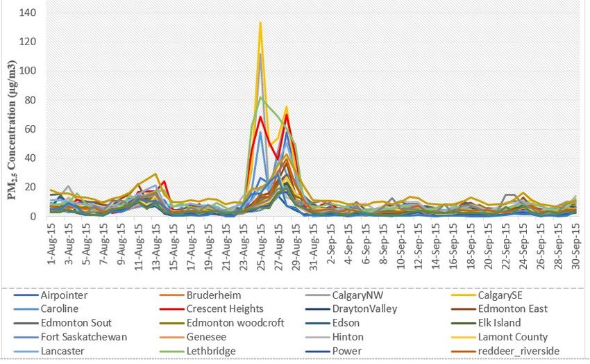
Atmosphere 2018, 9, 335                                                                             3 of 18

Remote sensing observations, including AOD images, provide extensive spatial coverage and reliable
repeated measurements. However, there are some limitations with AOD images. For example,
cloudy days are a major problem with remotely sensed methods of PM2.5 estimation [24], as they limit
the number of days available for analysis.
      A variety of satellite sensors provide AOD image including Moderate Resolution Imaging
Spectrometer (MODIS), the Ozone Monitoring Instrument (OMI), the Multi-Angle Imaging
Spectrometer (MISR), the Geostationary Operational Environment Satellite (GEOS), Polarization of
Earth’s Reflectance and Directionality (POLDER), the Sea-viewing Wide Field-of-view Sensor (SeaWiFS),
and the Cloud-Aerosol Lidar with Orthogonal Polarization (CALIOP). AOD is affected by ambient
conditions, such as humidity and vertical profile, as well as chemical properties of the atmosphere [45].
      Land use regression (LUR) methods estimate pollution concentration at a given location using
surrounding attributes, such as land use type and traffic characteristics within a surrounding area,
as predictors [33]. LUR is generally used to estimate air pollution at fine spatial scales, and can be
used to assign household-level exposure in community health studies [20]. Based on the type of
the pollutant and the source of the air pollution different land use variables can be used in LUR.
For example, road types, parks, residential, commercial, and industrial land uses have been used by
Bertazzon et al. (2015), for modeling urban air pollution [20]. Yang et al. (2017) developed LUR to
estimate PM2.5 and NO2 using different land use types including cultivated land, forest, grassland,
shrub and water land, and traffic and urbanization [46]. According to a report by Environment and
Climate Change Canada (2017), the main sources of PM2.5 emission in Canada include dust and fire,
agriculture, home firewood burning, mineral and oil and gas industry, transportation, and building
utilities [47]. Different specifications of LUR (ordinary least squares (OLS) regression, geographically
weighted regression (GWR), and spatial autoregression (SAR)) have been employed to predict air
pollution in different studies [20,38,48].
      Different factors affect the identification of the most reliable models in different wildfire events
and areas. As each model has strengths and weaknesses, no single model can be considered the
most accurate to quantify human exposure to wildfire smoke [44]. For example, ground-based
measurements provide accurate information for each station; however, the spatial density of station
distribution is not sufficient to estimate the spatial distribution of wildfire smoke. GWR is suitable on
a reginal scale and needs small amounts of data; however, its performance depends on ground-based
measurements. Therefore, in areas lacking air quality (AQ) stations, GWR is not reliable [44]. CTM can
predict pollutant concentration without ground based measurements [49]. However, collecting the
necessary chemical and physical information is time consuming and requires financial resources [50].
Although MLR has relatively weak predictability, it can be improved by adding some covariates [44].
For example, for estimating PM2.5 using AOD aerosol type, methodological and land use variables
may be included in the regression to improve the model performance [28,51,52]. MEM performance is
usually strong, and the R2 value could reach up to 0.80 [27,53]. The main disadvantage of this method
is that, if ground-based stations are not available in some areas, the model assumptions are not met,
potentially affecting its performance [54]. In addition, there are differences between models trained for
smoke-based PM2.5 (i.e., when the wildfire is the source of PM2.5 ), and models developed to estimate
PM2.5 from other sources, mainly of industrial and transportation origin.
      In the present study, the model choice was affected by many factors, including the number of
ground-based AQ monitors, the characteristics of the study area, data availability, data uncertainty,
and the significance of spatial autocorrelation in the data. Experiments with a range of predictors
showed that the predictors associated with PM2.5 could change even over a short period (two months),
depending on the source of PM2.5 . The predictors considered include spatial and temporal variables,
such as wind speed and land use variables, and satellite data, including AOD and (normalized difference
vegetation index). Roadway and industrial variables are established predictors in LUR models for
estimating air pollution [17,19,55], whereas satellite observations are relatively uncommon. In the
present study, we investigated the role of vegetation on the level of PM2.5 concentration during a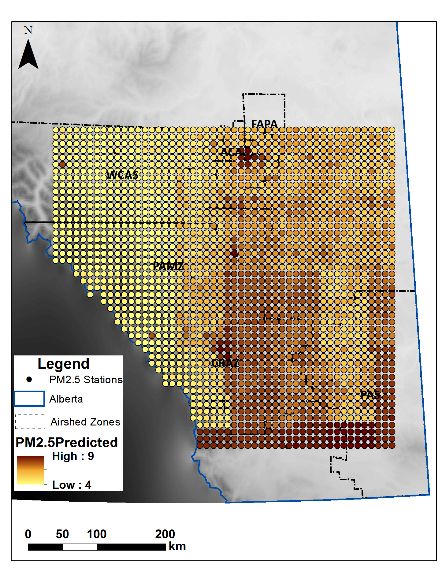
Atmosphere 2018, 9, 335 4 of 18
wildfire event. Plants have the ability to reduce some of air pollution particles as plant leaves and
stems increase surface areas to which airborne particles can be absorbed [56]. NDVI is an index
of greenness, vegetation, and agriculture land use that has been rarely used as a predictor in LUR
models [57–60]. Wu et al., [57] investigated the role of surrounding greenness on intra urban PM2.5
variability, showing that there was a strong negative correlation (ranging between −0.71 and −0.77)
between NDVI and PM2.5 .
To examine
Atmospherethe
2018,temporal
9, x FOR PEERvariability
REVIEW in predictors, we divided the study period into4 ofthe 18 following
three sub-periods. “Pre-fire period”, that is, when the level of PM2.5 in the study area was normal
predictor in LUR models [57–60]. Wu et al., [57] investigated the role of surrounding greenness on
(the average 3 [60]); “during-fire”
intralevel
urbanof PM the 24-h PM showing
2.5 variability, 2.5
was lower
that therethan
wasthe standard
a strong negative level: 30 µg/m
correlation (ranging between
period, that is,and
−0.71 when−0.77)the concentration
between NDVI and PM of2.5PM
. 2.5 was dramatically increased in the majority of AQ
stations locatedToinexamine
the study the area;
temporal variabilityperiod,
“post-fire" in predictors,
that is,we divided
when the the
PMstudy period into the
2.5 concentration returned to
following three sub-periods. “Pre-fire period”, that is, when the level of PM2.5 in the study area was
background levels. The subdivision of the study period into three separate sub-periods allowed us to
normal (the average level of the 24-h PM2.5 was lower than the standard level: 30 µg/m3 [60]); “during-
test different models for the same study area, yet with very different
fire” period, that is, when the concentration of PM2.5 was dramatically increased PM 2.5 in the majority oflevels and
concentration
pollutant sources
AQ stations over two months.
located in the study The study
area; area covers
“post-fire" period, most
that is,ofwhen
southern
the PM Alberta, including urban
2.5 concentration
and rural returned to background
areas. Rural levels. The
areas usually havesubdivision
insufficientof theAQ
study period into
monitors three
and separate
most sub-periods
epidemiological studies
allowed us to test different models for the same study area, yet with very different PM2.5
are limited to urban areas. We propose an extension of the models to rural areas to estimate levels of
concentration levels and pollutant sources over two months. The study area covers most of southern
smoke-based PMincluding
Alberta, 2.5 concentration in areas
urban and rural areas. where AQusually
Rural areas monitors are not enough
have insufficient or available.
AQ monitors and most
In theepidemiological
present study, we are
studies estimate two
limited to urbantypes ofWe
areas. predictive
propose anmodels:
extension univariate
of the modelsmodels
to rural based on
areas to estimate levels of smoke-based PM 2.5 concentration in areas where AQ monitors are not
satellite AOD; and integrated AOD-LUR models. Both models yield estimates of PM2.5 for each of the
enough or available.
sub-periods in August and September 2015 over the whole urban and rural southern Alberta.
In the present study, we estimate two types of predictive models: univariate models based on
satellite AOD; and integrated AOD-LUR models. Both models yield estimates of PM2.5 for each of the
2. Materials and Methods
sub-periods in August and September 2015 over the whole urban and rural southern Alberta.
2.1. Study 2.Area and Ground-Level
Materials and Methods PM2.5 Measurements (Dependent Variable)
The study area
2.1. Study Areacovers the southern
and Ground-Level part of the
PM2.5 Measurements province
(Dependent of Alberta (Canada). The Clean Air
Variable)
Strategic Alliance
The study area covers the southern part of the province of Albertain(Canada).
(CASA) was established to manage air quality Alberta.TheTen Airshed
Clean Air zones
were formed between 1996 and 2017; the study area includes six of these zones:
Strategic Alliance (CASA) was established to manage air quality in Alberta. Ten Airshed zones wereAlberta Capital
formed between
Airshed (ACA), Calgary1996 and 2017;
Region the study
Airshed area(CRAZ),
Zone includes six of these
Fort zones: Alberta Capital
Air Partnership (FAP),Airshed
Palliser Airshed
(ACA), Calgary Region Airshed Zone (CRAZ), Fort Air Partnership (FAP), Palliser Airshed Society
Society (PAS), Parkland Airshed Management Zone (PAMZ), and West Central Airshed Society (WCAS)
(PAS), Parkland Airshed Management Zone (PAMZ), and West Central Airshed Society (WCAS)
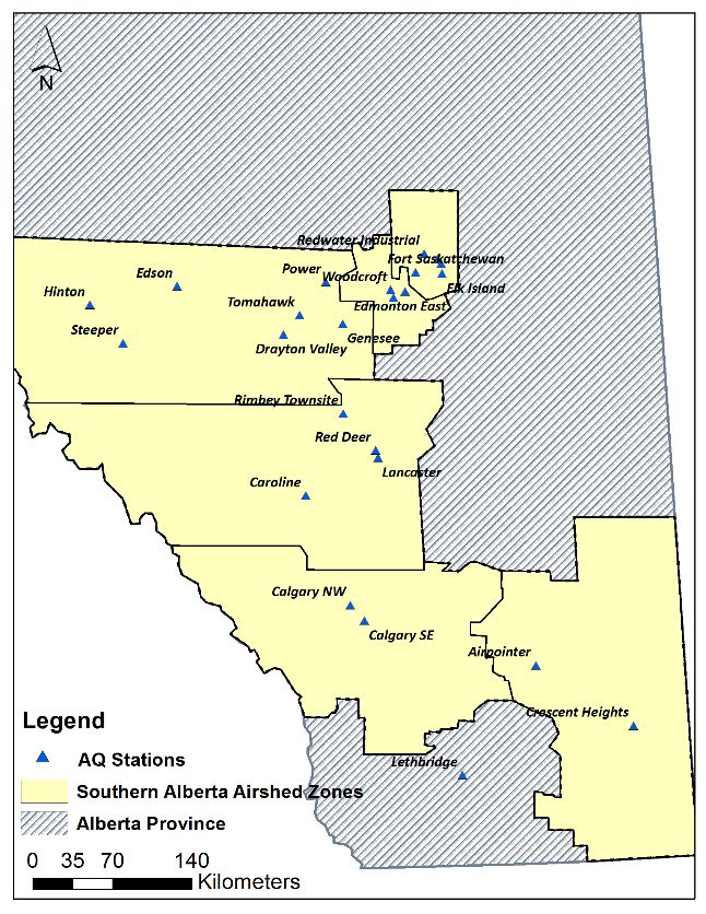
(Figure 1).(Figure
The Airshed zoneszones
1). The Airshed nownowoperate
operatemore
more than 70airair
than 70 monitoring
monitoring stations
stations across
across the the Province.
Province.
(a) (b)
Figure 1. Alberta airshed zones (a) (www.albertaairshedscouncil.ca), Distribution of 24 monitoring
Albertainairshed
Figure 1. stations zones
the Southern (a) airshed
Alberta (www.albertaairshedscouncil.ca),
zones used in the present study (b).Distribution of 24 monitoring
stations in the Southern Alberta airshed zones used in the present study (b).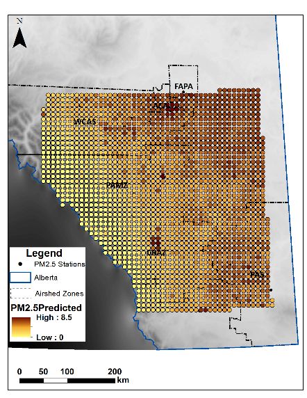
Atmosphere 2018, 9, 335                                                                           5 of 18

     Twenty-four-hour PM2.5 concentrations were collected at 24 Alberta Airshed Zones continuous
AQ stations (Figure 1b) for the months of August and September 2015 (http://airdata.alberta.ca/
RelatedLinks.aspx). The daily PM2.5 concentrations were averaged for each period in each station.

2.2. Temporal (Meteorological) and Spatial Predictors
      Wind speed and direction were collected at each monitoring station. A windrose was created
using four quadrants, defined by radii traced at 0, 90, 180, and 270 degrees, so that each quadrant
is centered on the northeast, southeast, southwest, and northwest directions, respectively. As the
fire source is located southwest of the study area, based on the recorded wind direction, hourly
wind speed, the southwest quadrant of each station was averaged over each of the three sub-periods.
Average humidity and temperature over each period were obtained from continuous weather stations
as well.
      Industrial and road length predictors were generated by drawing circular buffers around each
monitoring station. Following the previous studies [20], the buffers for industrial variables ranged
from 5000 to 10,000 m and for road length from 500 to 1000 m. The number of industrial emission
points and length of road in each buffer were calculated. The Alberta road network was acquired
from the National Road Network (NRN) [61], and industrial points were obtained from the National
Pollutant Release Inventory (NPRI) [62].
      Elevation data were acquired through an Alberta DEM (digital elevation model) from DMTI
Spatial [63]: Contour lines, stored in a shapefile, were converted to a raster file of elevation values,
using ESRI ArcMap 10.3.1.
      As the 2015 PNW wildfire originated in Washington State, USA, the centroid of the fire was
digitized in ArcGIS as a source of the smoke over Alberta. The Euclidean distance between each AQ
station in the study area and the source of the fire was calculated.

2.3. Satellite Data

2.3.1. Satellite AOD Images
     One of the most common satellite products used in the field of air quality is aerosol optical
depth (AOD), a quantity that indicates the amount of aerosol particles in the atmosphere. In our study,
AOD data were derived from both MODIS and ozone monitoring instrument (OMI).
     Averaged MOD 08 product of MODIS (at 1 degree resolution) and OMI/Aura AOD data
(at 0.25 degree resolution) were collected from the NASA Giovanni website [64] for the three
sub-periods (pre-, during, and after-fire) of the study.

2.3.2. NDVI
     Normalized Difference Vegetation Index (NDVI) has been used as greenness predictor in previous
air pollution studies [57–60]. NDVI is an image-based greenness index for measuring and monitoring
density of plant, vegetation and biomass production on the earth. The NDVI values range is from
−1 to +1. Increasing positive NDVI values indicate increasing amount of healthy vegetation and
correspond to dense vegetation. Areas covered by rock, sand, snow, and non-vegetative features show
very low NDVI values (close to -1).
     Global NDVI is one of the vegetation products of MODIS that contains atmospherically corrected
bi-directional surface reflectance. Global NDVI data are provided every 16 or 30 days. In the present
study, MOD13C2 data (monthly NDVI image) were downloaded from the NASA Giovanni website [64].
Considering that the NDVI is not expected to change significantly over a month we collected one
image for August 2015 and one for September 2015. Those monthly NDVI images were projected on a
0.05 degrees geographic Climate Modeling Grid (CMG).
Atmosphere 2018, 9, 335                                                                              6 of 18

2.4. PM2.5 Predictive Models
     In the present study, a univariate model was first tested, using AOD as the single predictor,
to assess the amount of variability of PM2.5 concentration that can be modeled by AOD for different
pollution levels in each sub-period. Subsequently, this simple model was integrated into a LUR model
by including traditional land use variables (Equation (1)) [20], as well as meteorological variables.
The purpose of this integration was to improve the model’s spatial and temporal fit, as the relationship
between AOD and PM2.5 is thought to be affected by other variables. Furthermore, the latter model tests
the association of PM2.5 with relevant predictors. An AOD-LUR multivariate model was independently
estimated for each sub-period. Model selection led to the identification of different sets of significant
predictors, yielding respective coefficients for each sub-period.
     Traditional LUR models are defined as:

                                         yi = β 0 + ∑ β k xik + ε i                                     (1)
                                                     k

where the response variable, y, (e.g., PM2.5 ) indicates pollution concentration at location i, (where each
i is a sample AQ station), and is expressed as a function of k attributes, or independent variables (x),
such as land use variables and traffic characteristics [33]. Coefficients are estimated using the ordinary
least squares (OLS) estimation method.
      Variable selection was conducted independently for each sub-period model; over twenty
variables were tested in the prediction models, including spatial predictors (land use type,
industrial, and transportation indicators), temporal predictors (meteorology) and remotely sensed data
(AOD and NDVI). Model selection was based on theoretical relevance and statistical significance. First,
the most relevant variables were chosen for initial list in each period. Then, forward stepwise multiple
linear regression and subset regression methods were used to identify the most significant predictors
in each model. Global Moran’s I [65] was used to identify spatial clustering and autocorrelation at
the spatial variables, i.e., PM2.5 , land use variables, and satellite observations recorded at each AQ
station. Residual Moran’s I and Lagrange multiplier (LM) test [66] were used to assess the spatial
autocorrelation in the residuals of each sub-period model.
      After estimating the best prediction model for each sub-period, the regression coefficients were
applied to calculate PM2.5 in the centroid of each 10 by 10 km grid-cell overlaying the study area.
Then inverse distance weighted (IDW) interpolation technique was applied to map the calculated
PM2.5 level between grid centers. IDW works on the assumption that near things are more alike than
things that are farther apart. Using the estimated value at each grid center, IDW predicts a value for
any unknown location, giving greater weights to points closer to the known location. The weights
are determined by distance [67]. A summary of variables, their names, and additional details are
shown in Table 1. Performance of the models in the PM2.5 concentration estimation is evaluated
by using different statistical indices including coefficient of determination (R2 ), adjusted coefficient
of determination (adj R2 ), cross-validated R2 (CV-R2 ), RMSE, CV-RMSE, and Akaike information
criterion (AIC).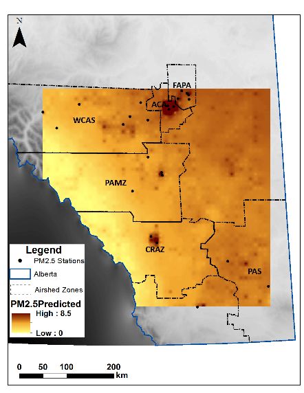
Atmosphere 2018, 9, 335                                                                                         7 of 18

      Table 1. Response (PM2.5 ) and predictor variables including satellite data, spatial and temporal
      variables used in variable selection procedure.

     Response Variable                   Name                           Unit
            PM2.5                Particulate Matter 2.5                µg/m3
       Satellite Data                    Name                    Spatial Resolution        Temporal Resolution
     Vegetation Index                NDVI-30 days                    0.05 degree                  Monthly
   Aerosol optical depth                                                                  Daily (averaged to study
                                     AOD_MODIS                         1 degree
        (MODIS)                                                                                    period)
   Aerosol optical depth                                                                  Daily (averaged to study
                                        AOD_OMI                      0.25 degree
          (OMI)                                                                                    period)
     Spatial Variables                   Name                           Unit               Circular Buffer/Scale
  Distance to the source of
                                          Dis                         kilometer                        -
             fire
    Land use: Industrial                 LU_ind                         count                 5000–10,000 m
           roads                          Road                          meter                  500–1000 m
    Temporal Predictors                  Name                           Unit                       Resolution
                                                                                            Hourly (averaged to
     Relative Humidity                    RH
                                                                                               study period)
                                                                                            Hourly (averaged to
        Temperature                      Temp                          Celsius
                                                                                               study period)
                                                                                            Hourly (averaged in
  Wind speed (southwest)                  WS                     km/h, at 10 m height
                                                                                            southwest direction)

2.5. Validation
     The validity of the AOD-based and AOD_LUR models used for estimation of PM2.5 concentration
was evaluated by a cross-validation procedure. As the total number of AQ stations (PM2.5 samples) was
too small to divide the data set to test and train separately, we applied leave-one-out cross validation
(LOOCV) procedure. With this method, each PM2.5 measurements are estimated based on a model
calibrated over the other PM2.5 measurements. Therefore, in this study, for each period, we developed
almost 24 individual models (after removing outliers we had 22 data for pre-fire period, 24 data
for during-fire period, and 23 data for post-fire period). Then the cross-validated root mean square
error (CV-RMSE) and CV-R2 were calculated for validating the models. The structure of the model
(the variables in the model) was the same as the one used in the full training dataset (the model trained
by 24 PM2.5 measurements) but the coefficients of the model changed.

3. Results
     Table 2 shows the descriptive statistics of PM2.5 concentration over the three sub-periods.
The overall mean concentration of PM2.5 over the during-fire period is significantly higher than
the pre- and post-fire periods (i.e., 19.5 µg/m3 compared to 6.2 µg/m3 and 4.2 µg/m3 , respectively).
Global Moran’s I tests indicate that there was no significant spatial autocorrelation in the measured
PM2.5 at AQ stations in any of the sub-periods over the study area.

                      Table 2. Descriptive statistics of PM2.5 concentration over three periods.

         PM2.5 (µg/m3 )             N        Max       Mean          Min           S.D.    Moran’s I        P(I)
      Period 1 (Pre-Fire)          22         14          6.2         3.2          2.4        0.08           0.1
    Period 2 (During-Fire)         24        51.5         19.5         6           12.9       0.55          0.00
     Period 3 (Post-Fire)          23         9.8         4.2         0.8          2.1        0.01          0.28
Atmosphere 2018, 9, 335                                                                                                  8 of 18

     The temporal daily variability of PM2.5 level at each of the 24 AQ stations during the whole
period (1 August to 30 September) is shown in Figure 2. The recorded concentrations of PM2.5
increased greatly in late August. Calgary monitors reported the level of PM2.5 as about 170 µg/m3 on
25 August, which is, more than three times their typical peak in non-smoke days. It can be seen in this
figure that the daily averaged PM2.5 level for some stations was more than 80 µg/m3 on 25 August.
By 1 Atmosphere
     September,     the PM2.5 concentration
                2018, 9, x FOR PEER REVIEW
                                            returned to the background level.               8 of 18

               Figure 2. Temporal daily variability of PM2.5 level at the 24 stations located at the study area.
          Figure 2. Temporal daily variability of PM2.5 level at the 24 stations located at the study area.
         The spatial variability of PM2.5 concentration was estimated using AOD and AOD-LUR models
    during  the three
    The spatial        sub-periods.
                  variability of PMThat     is, two modelswas
                                      2.5 concentration     wereestimated
                                                                   developedusing
                                                                                for each
                                                                                      AODperiod.
                                                                                            and The   univariate
                                                                                                 AOD-LUR       models
    AOD   models   are summarized   in Table    3, and the multivariate AOD-LUR
during the three sub-periods. That is, two models were developed for each period. Themodels in Table 4. Theunivariate
                                                                                                            final
AODequation
     models ofarethe multivariate in
                   summarized     model
                                     Table for3,each
                                                 andsub-period   is as follows:
                                                       the multivariate   AOD-LUR models in Table 4. The final
         Pre-fire period model:
equation of the multivariate model for each sub-period is as follows:
    Pre-fire period model: = 3.84 + (4.82 ×     ) + (6.8 × 10 × Road                         )                     (2)
           During-fire period model:
                              yi = 3.84 + (4.82 × AOD ) + 6.8 × 10⁻⁵ × Road1km                                              (2)
                          = 63.38 + (12.71 ×        ) + (−32.95 × NDVI) + (−5.656 × 10            × Dist)          (3)
         Post-fireperiod
      During-fire period model:
                         model:
                 log( ) = 1.55 + (−9.61 × 10 ×            ) + (1.87 ×10 × Road ) + (2.9
                                                                                                                   (4)
               yi = 63.38 + (12.71 × AOD
                                × 10        ) + (−32.95
                                        × LU_ind_  )    × NDVI) + −5.656 × 10⁻⁵ × Dist                                      (3)
             As it is shown in the above equations, there are substantial differences between the intercept
      Post-fire period model:
      values across multivariate models. The highest intercept value was obtained for the during-fire
      period, due to the higher level of PM2.5 concentration in that period. The lowest intercept was
      obtained for the  post-fire period, as we applied
                                                      a logarithmic transformation
                                                                                    to PM2.5 to normalize
  log(the
       yi ) PM
            = 1.55  + −9.61 × 10⁻⁴ × Elevation + 1.87 × 10⁻⁵ × Road1km + 2.9 × 10⁻² × LU_ind _5km (4)
               2.5 distribution and improve the results.

     As it is shown in the above equations, there are substantial differences between the intercept
values across multivariate models. The highest intercept value was obtained for the during-fire period,
due to the higher level of PM2.5 concentration in that period. The lowest intercept was obtained
for the post-fire period, as we applied a logarithmic transformation to PM2.5 to normalize the PM2.5
distribution and improve the results.
Atmosphere 2018, 9, 335 9 of 18
Table 3. Results of aerosol optical depth (AOD)-based model for three periods.
Period 1: Pre-Fire (1–23 August 2015) Period 2: During-Fire (24–31 August 2015) Period 3: Post-Fire (1–30 September 2015)
Predictors
Coefficient Std. Error p-Value Coefficient Std. Error p-Value Coefficient Std. Error p-Value
Intercept 4.165 0.58 0.00 4.512 3.77 0.24 0.73 0.35 0.05
AOD 7.76 2.65 0.00 18.154 3.93 0.00 6.75 4.47 0.14
Index/Test Adjust/p-Value Index/Test Adjust/p Value Index/Test Adjust/p Value
R2 0.29 0.26 0.50 0.47 0.13 0.05
CV-R2 0.25 - 0.40 - 0.12 -
Moran’s I 0.09 0.05 0.05 0.07 −0.03 0.37
LMerr 0.54 0.46 0.23 0.62 0.08 0.76
RMSE 1.4 - 9 - 0.51 -
CV-RMSE 1.39 - 9.8 - 0.6 -
AIC 78 - 179 - 41 -
Table 4. Results of aerosol optical depth–land-use regression (AOD-LUR) model for three periods.
Period 1: Pre-Fire (1–23 August 2015) Period 2: During-Fire (24–31 August 2015) Period 3: Post-Fire (1–30 September 2015)
Predictors
1
cor (%) Coefficient Std. Error p-Value cor (%) Coefficient Std. Error p-Value cor (%) Coefficient Std. Error p-Value
Intercept - 3.84 0.58 0.00 - 63.38 13.08 0.00 - 1.55 0.44 0.00
AOD 0.50 4.82 2.75 0.09 0.70 12.71 3.00 0.00 - - - -
NDVI - - - - 0.60 −32.95 9.61 0.00 - - - -
Distance - - - - 0.61 −5.6 × 10⁻⁵ 0.00 0.00 - - -
−9.61 ×
Elevation - - - - - - - - 0.35 0.00 0.05
10−4
Road_1km 0.55 6.8 × 10⁻⁵ 0.00 0.00 - - - - 0.50 1.87 × 10⁻⁵ 0.00 0.00
LU_ind_5km - - - - - - - - 0.51 2.9 × 10⁻² 0.01 0.08
Index/Test Adjust/p-Value Index/Test Adjust/p-Value Index/Test Adjust/p-Value
R2 0.50 0.45 0.77 0.74 0.54 0.47
CV-R2 0.41 - 0.71 - 0.42 -
Moran’s I −0.028 0.35 0.04 0.01 −0.16 0.83
LMerr 0.051 0.82 0.12 0.72 1.84 0.17
RMSE 1.17 - 6 6.8 0.36 -
CV-RMSE 1.34 - 7.06 - 0.44 -
AIC 77 - 162 - 29 -
1: Correlation between PM2.5 and predictors in each period.Atmosphere 2018, 9, 335 10 of 18
Atmosphere 2018, 9, x FOR PEER REVIEW 10 of 18
The
Themodel
model results shown in
results shown in Table
Table33forforall
allthree
threesub-periods
sub-periods indicate
indicate that
that thethe goodness-of-fit
goodness-of-fit of
of the
the univariate AOD model was limited, especially for the pre- and post-fire periods,
univariate AOD model was limited, especially for the pre- and post-fire periods, that is, when the PM2.5 that is, when the
PM 2.5 level was low. The goodness-of-fit for all three sub-periods improves substantially by adding
level was low. The goodness-of-fit for all three sub-periods improves substantially by adding temporal
temporal
and spatial andvariables
spatial variables to each regression
to each regression (Table 4). (Table
The 4).
LUR Thewas
LUR was developed
developed for eachforperiod
each period
using
using different image-based, temporal, and spatial variables. The only
different image-based, temporal, and spatial variables. The only significant variable, beside AOD, significant variable, beside
in the
AOD, in the pre-fire model is “road length within a 1000-m buffer”. With the
pre-fire model is “road length within a 1000-m buffer”. With the addition of this variable, the model addition of this variable,
the
R2 model
increasedR2 increased
from 0.29from 0.29 For
to 0.50. to 0.50.
the For the during-fire
during-fire model, model, the significant
the significant variables,
variables, besides besides
AOD,
AOD, were “NDVI”, and “distance to fire. The integration of AOD with
were “NDVI”, and “distance to fire. The integration of AOD with distance to the fire period and distance to the fire period
and
NDVI NDVI improved
improved modelmodel performance
performance substantially,
substantially, as shown as by
shown by the
the higher R2higher
value ofR2the
value of the
AOD_LUR
AOD_LUR model compared to AOD-based model (AOD-LUR’s
2 R
model compared to AOD-based model (AOD-LUR’s R = 0.77 verses AOD-based model’s R = 0.50),
2 = 0.77 verses AOD-based model’s 2
Ralong
2 = 0.50), along with lower AIC and RMSE values for the AOD-LUR model compared to AOD-based
with lower AIC and RMSE values for the AOD-LUR model compared to AOD-based model
model
(AOD_LUR’s(AOD_LUR’s AIC andAIC and RMSE
RMSE = 162 and= 162 6, and
verses6, verses
AOD-basedAOD-based
model’s model’s
AIC and AIC and RMSE
RMSE = 179 and = 179
9).
and 9). For the post-fire model, significant variables were “elevation”, “road
For the post-fire model, significant variables were “elevation”, “road length within a 1000-m buffer”, length within a 1000-m
buffer”, and “industrial
and “industrial land useland
withinuseawithin
5000-ma buffer”.
5000-m buffer”.
As shown Asin shown
Tablesin3Tables
and 4, 3AODand did
4, AOD did not
not perform
perform well in the post-fire period. For most periods, the
2 CV-R 2 was less than 10% lower than the
well in the post-fire period. For most periods, the CV-R was less than 10% lower than the model
model
adjusted adjusted
R2 . ForR2. example,
For example,in thein the during-fire
during-fire period
period thethe multi-variatemodel
multi-variate modelRR22 andand CV-R
CV-R2 were
2
were
0.74
0.74 and
and 0.71
0.71 respectively,
respectively, less
less than
than 5%5% decrease
decrease in in CV-R
CV-R2 (Table
2
(Table 4).
4). This
This model
model showed
showed the the best
best
performance
performancebased based onon validation
validation methods.
methods.
Residual
ResidualMoran’s
Moran’sII and
and Lagrange
Lagrange multiplier
multiplier(LMerr)
(LMerr)teststestsfor
for all
all three
three periods
periods indicated
indicated thatthat
there is no significant spatial autocorrelation in any of the model residuals. Therefore,
there is no significant spatial autocorrelation in any of the model residuals. Therefore, geographically geographically
weighted
weighted or or spatially
spatially autoregressive
autoregressive models
models were were notnot deemed
deemed necessary.
necessary.
PM
PM2.52.5Predictive
PredictivePM
PM2.52.5Maps
Maps
To
Toextend
extendthetheestimation
estimationofofPM PM2.5 to to
2.5 the entire
the study
entire area,
study a 10a by
area, 10 10
bykm gridgrid
10 km waswas
overlaid to the
overlaid to
study area. First, the value of the model’s variables at the center of each grid cell was
the study area. First, the value of the model’s variables at the center of each grid cell was extracted, extracted, and
then, by using
and then, the developed
by using the developedmodels
models for for
each sub-period
each (shown
sub-period (shown in in
Table
Table4 4and
andEquations
Equations(2)–(4)),
(2)–(4)),
the
thePM
PM2.52.5levels
levelswere
werecalculated
calculatedatateach
eachgridgridcenter.
center.An
AnIDW
IDWinterpolation
interpolationtechnique
techniquewaswasapplied
appliedtoto
interpolate the PM level between grid centers. The predictive maps are shown
interpolate the PM2.5 level between grid centers. The predictive maps are shown in Figure 3.
2.5 in Figure 3.
(a) (b) (c)
Figure 3. Cont.Atmosphere 2018, 9, 335 11 of 18
Atmosphere 2018, 9, x FOR PEER REVIEW 11 of 18
(d) (e) (f)
Figure 3. The predicted PM2.5 maps over the study area including: Prediction results obtained by
Figure 3. The predicted PM2.5 maps over the study area including: Prediction results obtained by
models’ coefficient at grid centroid (a–c), and interpolated maps between grids (d–f), for the three
models’ coefficient at grid centroid (a–c), and interpolated maps between grids (d–f), for the three
periods separately: (a,d) Pre-fire predicted maps, (b,e) during-fire predicted maps, and (c,f) post-fire
periods separately: (a,d) Pre-fire predicted maps, (b,e) during-fire predicted maps, and (c,f) post-fire
predicted maps.
predicted maps.
4. Discussion
4. Discussion
4.1.
4.1.Relation
Relationbetween
betweenAOD
AODand
andPM
PM2.5 Based on Different Smoke Levels
2.5 Based on Different Smoke Levels
The
The results
results of
of both
both AOD AOD andand AOD-LUR,
AOD-LUR, for for all
all periods,
periods, indicate
indicate that
that with
with lower
lower level
level of PM2.5
of PM 2.5
concentration,
concentration, the predictive ability of AOD in the models decreased. Studies have shown that
the predictive ability of AOD in the models decreased. Studies have shown that
satellite
satelliteAOD
AODisiswell
wellsuited
suitedfor fordetecting
detectinglarge largechanges
changesin inaerosol
aerosolcontent
content[36],
[36],which
whichcan canexplain
explainthe the
higher performance of the during-fire models compared to pre- and
higher performance of the during-fire models compared to pre- and post-fire models. The increasedpost-fire models. The increased
level
level of
of PM
PM2.5 concentration increases the correlation between AOD and PM2.5, leading to a better
2.5 concentration increases the correlation between AOD and PM2.5, leading to a better
model
model performance.
performance. The The graph
graph inin Figure
Figure 22 demonstrates
demonstrates the the difference
difference inin PMPM2.5 concentration in the
2.5 concentration in the
during-fire period compared to the other two periods, and it can be seen
during-fire period compared to the other two periods, and it can be seen from the graph that there from the graph that there is
also a small peak in the pre-fire period between 11 and 15 August. It
is also a small peak in the pre-fire period between 11 and 15 August. It is clear from both uni- and is clear from both uni- and
multivariate
multivariatemodels
modelsthat thatthetheAOD
AODmodelsmodelsimproved
improvedwhen whenthe thesmoke
smokefromfromthe thewildfire
wildfiredrifted
driftedoverover
the study area, leading to a high level of PM 2.5. However, both for the pre- and post-fire periods, when
the study area, leading to a high level of PM2.5 . However, both for the pre- and post-fire periods,
the
whenlevels of PMof
the levels 2.5 were fairly low, the model performance decreased due to the lower correlation
PM2.5 were fairly low, the model performance decreased due to the lower correlation
between
between AOD andPM
AOD and PM2.52.5(mean
(meanPM PM 2.5 = 4.2 µg/m3 compared3 to 6.2 µg/m3 and3 19.5 µg/m3 for pre- 3 and
2.5 = 4.2 µg/m compared to 6.2 µg/m and 19.5 µg/m for pre-
during-fire periods).
and during-fire periods).
The
The main
main difference between the
difference between thepost-fire
post-firemodelmodelverses
versespre-pre- and
and during-fire
during-fire models
models waswasthatthat
the
the AOD showed little correlation with PM 2.5 level and it was not significant either in the univariate
AOD showed little correlation with PM2.5 level and it was not significant either in the univariate model
model or integrated
or in the in the integrated
AOD-LUR AOD-LUR
model.model. The relatively
The relatively weak weak
resultsresults obtained
obtained by theby the AOD-model
AOD-model in the
in the post-fire period, compared to the pre- and during-fire period, may
post-fire period, compared to the pre- and during-fire period, may be due to uncertainties in MODIS be due to uncertainties in
MODIS AOD data, such as cloudy days. In southern Alberta, the month
AOD data, such as cloudy days. In southern Alberta, the month of September experiences gradually of September experiences
gradually
increasingincreasing
cloud cover. cloud Forcover.
example, For example,
the percentage the percentage
of time that of time thatisthe
the sky sky is
mostly mostlyincreases
cloudy cloudy
increases
from 42%from to 47%42% in to 47% in37%
Calgary, Calgary,
to 44% 37% to 44% in Lethbridge,
in Lethbridge, 44% to 48% 44% to 48%
in Red Deerinbetween
Red Deer1 between
September 1
September and 30 September [68] . The increasing number of cloudy
and 30 September [68] . The increasing number of cloudy days in September (the post-fire period) days in September (the post-fire
period) have affected
have affected the performance
the performance of the model of the model
using AOD using
imageAOD due image
to thedue to the uncertainty
uncertainty in the AOD indata.
the
AOD data.
4.2. Selected Predictor Variables
4.2. Selected Predictor Variables
Although all three sub-periods used the same study area with almost the same AQ monitoring
Although all three sub-periods
stations for developing the multivariate usedmodels,
the same study
each finalarea
model with almost athe
included same AQ
different set monitoring
of variables.
stations for developing the multivariate models, each final model
The variable selection of the integrated AOD-LUR models highlights one key finding of included a different set of this
variables.
study:
The variable selection of the integrated AOD-LUR models highlights one key finding of this study:
The predictors of PM2.5 vary even over a short period of time (two months), as a function of theAtmosphere 2018, 9, 335 12 of 18
The predictors of PM2.5 vary even over a short period of time (two months), as a function of the
presence/absence of wildfire smoke. For example, for the pre-fire period, the variable selection
methods identified two variables: AOD, and road length on a 1000-m buffer. By adding the road length
variable to the AOD-based regression, the model’s R2 value increased from 0.29 to 0.50, emphasizing
the major impact of traffic emissions, especially in urban areas. The predictive ability of the during-fire
model using both AOD and AOD-LUR model was greater than pre- and post-fire models.
4.3. Relation between PM2.5 and NDVI
The negative correlation of −0.60% between NDVI and PM2.5 in the during-fire model (Table 4)
indicates that with an increased amount of vegetation, that is, plants and trees around the ground
monitoring stations, the level of PM2.5 decreases. Trees have the ability to reduce significant amounts
of ambient air pollutants, by primary absorbing pollution components via leaf stomata and plant
surface, and also by intercepting airborne particles [56]. Most of the intercepted particles are retained
on the plant surface [56]. The significantly higher coefficient of NDVI in the AOD-LUR model (in
absolute value) than the coefficients of the other variables may also indicate the essential role of plants
and vegetation in controlling wildfire-related PM2.5 level. Few studies have applied the greenness
index as a predictor in PM2.5 modeling. However, the role of vegetation and plants in reducing air
pollution during the fire events has not been assessed yet.
4.4. Relation between PM2.5 and Prevailing Wind Speed
The maps in Figure 3 show the spatial pattern of PM2.5 levels in the three sub-period and displays
a temporal pattern over the study period. This pattern appears to be associated with the source of
fire (south-west of Alberta) and prevailing wind direction that in the summer is from west to east
in most of Alberta. In the first period, when most of the study area’s monitoring stations showed
standard levels of PM2.5 , the predicted map shows an elevated level of PM2.5 in a small portion of
southern Alberta. In the rest of the study area, the road length variable is associated with the PM2.5
concentration, and, as it can be seen in the predictive map, the level of PM2.5 inside the cities is higher
than the level of PM2.5 in areas further out, where the road network is sparse.
During the fire period, the movement of the fire smoke to the interior portion of the study area
is clear: The north and northeast portions of the study area, that are farther from the source of fire are
still clean compared to its south and south-west portions.
The PM2.5 pattern in September, just after the fire, shows higher PM2.5 concentration in east and
northeast areas and lower in west and southwest areas. Even though we used coarse resolution AOD
images, the correlation of AOD and PM2.5 in two of the three sub-periods exhibited the highest value
among all predictors, and it was a one of the most significant predictors of PM2.5 .
Wind speed was not significant in any of the models, but it is interesting to note that the correlation
between PM2.5 concentration and wind speed during the fire had opposite signs, in comparison to
pre- and post-fire period (correlation between wind speed (at during-fire period) and PM2.5 = 0.60
and correlation between wind speed-pre/post-fire and PM2.5 = −0.15). The strong positive correlation
between wind speed and PM2.5 concentrations in the during-fire period is due to the prevailing wind
direction in southern Alberta. As the prevailing wind direction during the summer is from west to
east in most of Alberta, and the fire was located south-west of Alberta, the higher wind during the
fire would result in higher PM2.5 concentration. Conversely, in the pre-and post-fire periods the wind
helps to scatter the pollution and there was a negative correlation between wind speed and PM2.5 , and
low winds allow PM2.5 levels to rise [69].
4.5. Spatial Autocorrelation between AQ Measurements
PM2.5 over AQ stations did not exhibit significant spatial autocorrelation, nor did any of the
model residuals. This result is consistent with the known characteristics of PM2.5 : A regional pollutant,
which tends to exhibit little spatial variation. However, as spatial autocorrelation is an indicationAtmosphere 2018, 9, 335 13 of 18
of self-similarity over short distances, it would be a reasonable expectation during a wildfire event.
Non-significant spatial autocorrelation may be related to a smooth pollution pattern, driven by wind
and elevation, but it could also be a function of the relatively large distance between the AQ stations.
Owing to non-significant spatial autocorrelation in model residuals, reliable result estimates can be
obtained from simple linear (OLS) models.
4.6. Validating the Models by Leve-One-Out Cross Validation Procedure
As we mentioned before, the limitation of the present study was the limited number of AQ
stations. Therefore, it was not possible to have a separate dataset to validate the models. So, the models’
performance was evaluated using a leave-one-out cross validation method. Comparing R2 and adjusted
R2 of the full training dataset model with the CV-R2 shows small decrease in most of the models
(between 5% and 10%), which may indicate the reliability of the performance of the models and the
generalization ability of the models for a new data set.
Further support for the usefulness of most of the developed models, especially multivariate
models, is that both RMSE and CV-RMSE were low compared to the range in measured PM2.5
concentrations (Tables 2 and 4).
We can then say that the validation results indicate that the calibrated proposed models,
especially during-fire models could be used to estimate PM2.5 for other fire events in Southern Alberta.
4.7. Application of Integrated AOD-LUR Models in Rural Area
Most studies focus on urban areas due to the lack of AQ monitors in rural area as well as to
higher air pollution in urban areas resulting from human activities. The present study estimated
wildfire-related PM2.5 , as it relates to source of fire, as opposed to fossil fuel emissions in both urban
and rural areas. The results demonstrate that the use of satellite imagery and other land-use (LU)
variables can produce a model that might be useful in areas that suffer from the scarcity of AQ
monitors. Our study area, southern Alberta, despite including eight airshed zones, only has 24 AQ
monitors that measured PM2.5 , most of them located in urban areas. By incorporating MODIS AOD
and LU variables, we developed three models for three periods that estimated PM2.5 in both urban
and rural area. Even though the sparseness of AQ stations remains problematic, the proposed models
yield preliminary estimates of air pollution at relatively fine spatial resolution in rural areas. Hence,
epidemiological studies could use our model results to assess PM2.5 effect on human health in both rural
and urban areas. Further, these predictive models are applicable to other wildfire events, and could
help health authorities estimate the spatial and temporal pattern of smoke, with relative accuracy, in
major wildfire events.
5. Conclusions
In summary, we proposed a method applicable globally and regionally, which integrates the
use of MODIS AOD data into LUR models to identify smoke (particulate matter) concentration.
Univariate AOD and multivariate AOD-LUR models were developed to estimate the level of PM2.5
concentration in three different sub-periods: Pre-, during-, and post-fire. The AOD model performed
substantially better when combined with other covariates during the fire period, compared to the
univariate AOD model. The predictors in each period varied as a function of the sources of PM2.5 .
The three different sub-periods exhibited very large differences in PM2.5 concentration levels, as well as
in the source of PM2.5 . For this reason, separate models were developed for each sub-period. The three
univariate models differ from each other in the coefficients, goodness of fit, and other regression
diagnostics. The integrated multivariate AOD-LUR models further differ from each other in that each
model contains its own set of predictors, with their own associated coefficients.
In addition, our model estimated PM2.5 concentration at finer spatial scale compared to
ground-based measurements available from Alberta airshed zones, which exhibit a sparse distribution
of AQ monitors, far from sufficient for public health and epidemiological studies. The spatial andAtmosphere 2018, 9, 335 14 of 18
temporal estimates yielded by these models are particularly useful in rural areas, where such estimates
are rarely available. Furthermore, the model estimates can aid health authorities predict wildfire
smoke exposure at fine spatial and temporal scale, allowing them to better plan for wildfire events,
which are likely to increase in frequency and intensity as climate changes.
The result of this study could also be used in epidemiological studies to assess health effects
of smoke-related particulate matter during wildfire events, in contrast with those of particulate
matter pollution originating from other sources. The results improved the spatial accuracy and
reliability of the estimation of wildfire-related PM2.5 , enabling epidemiological studies to assess the
association between PM2.5 and smoke-related health effects during wildfire episodes. To this end,
it is essential for epidemiological studies to distinguish between wildfire-related PM2.5 and PM2.5
originating from other sources [15]. An important contribution of this paper is the comparison of
PM2.5 level during-fire events, in contrast to pre-fire and post-fire periods. Distance from the wildfire
is a significant predictor of PM2.5 during the fire event, in contrast with the pre- and post-fire period,
when the main predictors are transportation and industrial activities. Therefore, by estimated pre and
post PM2.5 maps, the PM2.5 related health effects before and after fire periods can be evaluated and
compared with smoke-related disease.
Further directions of enquiry include the calibration of the proposed models to estimate PM2.5
for other fire events, in southern Alberta and other regions. We plan to experiment with the use of
different satellite AOD data, to obtain even greater spatial accuracy, through the use of finer resolution
AOD, which will allow for filling the current MODIS AOD gaps.
Author Contributions: Conceptualization, M.M. and S.B.; Data curation, M.M.; Formal analysis, M.M. and I.C.;
Investigation, M.M., S.B. and I.C.; Methodology, M.M. and S.B.; Software, M.M.; Supervision, S.B.; Validation,
M.M., S.B. and I.C.; Writing—original draft, M.M.; Writing—review & editing, M.M., S.B. and I.C.
Funding: This research received no external funding.
Acknowledgments: We would like to acknowledge Roland Ngom and Vineet Saini for their support and
contribution to the project. Mojgan Mirzaei wishes to thank “Eyes High Doctoral Recruitment Scholarship”
for supporting her doctoral work. Stefania Bertazzon wishes to thank the Canadian Institutes for Health Research
(CIHR) Institute for Population and Public Health for funding the research on air pollution and public health.
We are grateful to our colleagues and members of the Geography of Health research group of the O’Brien Institute
for Population Health for their advice and insightful discussions. Finally, we would like to acknowledge the
anonymous reviewers for their constructive criticism and truly helpful comments.
Conflicts of Interest: The authors declare no conflict of interest.
References
1. Urbanski, S.P.; Hao, W.M.; Baker, S. Chapter 4 Chemical Composition of Wildland Fire Emissions.
Dev. Environ. Sci. 2008, 8, 79–107. [CrossRef]
2. California Air Resources Board, Health and the California Department of Public Wildfire Smoke A Guide for
Public Health Officials, California. 2011. Available online: https://oehha.ca.gov/media/wildfiresmoke2016.
pdf (accessed on 22 April 2018).
3. Reid, C.E.; Jerrett, M.; Tager, I.B.; Petersen, M.L.; Mann, J.K.; Balmes, J.R. Differential respiratory health
effects from the 2008 northern California wildfires: A spatiotemporal approach. Environ. Res. 2016, 150,
227–235. [CrossRef] [PubMed]
4. Johnston, F.H.; Henderson, S.B.; Chen, Y.; Randerson, J.T.; Marlier, M.; DeFries, R.S.; Kinney, P.;
Bowman, D.M.J.S.; Brauer, M. Estimated global mortality attributable to smoke from landscape fires.
Environ. Health Perspect. 2012, 120, 695–701. [CrossRef] [PubMed]
5. Kollanus, V.; Tiittanen, P.; Niemi, J.V.; Lanki, T. Effects of long-range transported air pollution from vegetation
fires on daily mortality and hospital admissions in the Helsinki metropolitan area, Finland. Environ. Res.
2016, 151, 351–358. [CrossRef] [PubMed]
6. Alberta Health Services. Wildfire Smoke and Your Health. 2018. Available online: https://myhealth.alberta.
ca/Alberta/AlbertaDocuments/wildfire-smoke-and-your-health.pdf (accessed on 5 July 2018).You can also read