A stochastic fractional dynamics model of space-time variability of rain - NASA
←
→
Page content transcription
If your browser does not render page correctly, please read the page content below
https://ntrs.nasa.gov/search.jsp?R=20140011340 2018-12-29T20:48:48+00:00Z

         JOURNAL OF GEOPHYSICAL RESEARCH: ATMOSPHERES, VOL. 118, 10,277–10,295, doi:10.1002/jgrd.50723, 2013

A stochastic fractional dynamics model of space-time
variability of rain
Prasun K. Kundu1,2 and James E. Travis 3
Received 17 December 2012; revised 7 August 2013; accepted 7 August 2013; published 18 September 2013.

[1] Rainfall varies in space and time in a highly irregular manner and is described naturally
in terms of a stochastic process. A characteristic feature of rainfall statistics is that they
depend strongly on the space-time scales over which rain data are averaged. A spectral
model of precipitation has been developed based on a stochastic differential equation of
fractional order for the point rain rate, which allows a concise description of the second
moment statistics of rain at any prescribed space-time averaging scale. The model is thus
capable of providing a unified description of the statistics of both radar and rain gauge data.
The underlying dynamical equation can be expressed in terms of space-time derivatives of
fractional orders that are adjusted together with other model parameters to fit the data. The
form of the resulting spectrum gives the model adequate flexibility to capture the subtle
interplay between the spatial and temporal scales of variability of rain but strongly
constrains the predicted statistical behavior as a function of the averaging length and time
scales. We test the model with radar and gauge data collected contemporaneously at the
NASA TRMM ground validation sites located near Melbourne, Florida and on the
Kwajalein Atoll, Marshall Islands in the tropical Pacific. We estimate the parameters by
tuning them to fit the second moment statistics of radar data at the smaller spatiotemporal
scales. The model predictions are then found to fit the second moment statistics of the gauge
data reasonably well at these scales without any further adjustment.
Citation: Kundu, P. K., and J. E. Travis (2013), A stochastic fractional dynamics model of space-time variability of rain,
J. Geophys. Res. Atmos., 118, 10,277–10,295, doi:10.1002/jgrd.50723.

1.       Introduction                                                      conveniently represented as suitable space and/or time ave-
                                                                           rages of a continuous stochastic field. This continuum appro-
  [2] Because of its irregular nature, rain is both difficult to            ximation is valid at the space-time resolution of the usual
measure accurately and predict from a physical model.                      measurement methods under normal rainy conditions in
Models of rain statistics provide a simple and conceptually                which the inherent discreteness of rain at the scale of individ-
economical way to capture the space-time variability of                    ual drops is smoothed out. In this paper we develop a phe-
precipitation in terms of a small number of adjustable para-               nomenological model of space-time statistics of rain in
meters. They can be relatively easily validated from a large               terms of a random field R(x, t) denoting the instantaneous
space-time data set, and once the parameters are tuned to                  point rain rate. It should be emphasized that R(x, t) is not
data, the model provides a rather efficient method of des-                  directly observable, but when suitably area- or time-averaged,
cribing various statistical properties of precipitation over               corresponds to measured quantities.
areas of similar rain climatologies.                                         [4] Radar scans yield area averages at an instant of time
  [3] In practice, rainfall is generally measured as a                     with horizontal spatial resolution of order 1 km. Rain gauge
(nearly) instantaneous area-averaged quantity in radar
                                                                           and disdrometer observations, on the other hand, lead to
measurements or as a time-averaged quantity at a point in
                                                                           time-averaged point rain rate estimates with temporal
rain gauge measurements. In theoretical models, they are
                                                                           resolution of order 1 min. These data can then be further
                                                                           “coarse-grained” by aggregating them to any desired larger
     1
                                                                           space-time scale. Although rainfall varies in an apparently
      Joint Center for Earth Systems Technology, University of Maryland,   irregular manner, the underlying physical processes take
Baltimore County, Baltimore, Maryland, USA.
    2
      Joint Center for Earth Systems Technology, NASA Goddard Space        place over an extended space-time region that causes the rain
Flight Center, Greenbelt, Maryland, USA.                                   rate field to be correlated in space and time. Moreover, the
    3
      Department of Mathematics and Statistics, University of Maryland,    statistics of rainfall depend on the space-time averaging
Baltimore County, Baltimore, Maryland, USA.                                scales in a nontrivial manner. In fact, it is well-known that
   Corresponding author: P. K. Kundu, Joint Center for Earth Systems       [see, e.g., Bell, 1987] there is a subtle interplay between
Technology, University of Maryland, Baltimore County, 5523 Research        the space-time scales associated with the decay of the corre-
Park Drive, Baltimore, MD 21228, USA. (prasun.k.kundu@nasa.gov)            lation function and the averaging scale that is reminiscent of
©2013. American Geophysical Union. All Rights Reserved.                    fluid turbulence. Like the velocity field of a turbulent fluid,
2169-897X/13/10.1002/jgrd.50723                                            the rain rate field R(x, t) has the property that the larger the

                                                                      10,277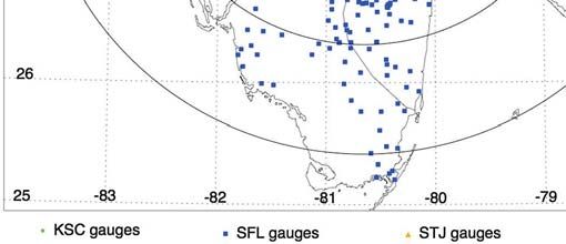
KUNDU AND TRAVIS: A SPECTRAL MODEL OF RAIN STATISTICS

averaging area, the longer the field remains temporally corre-        [7] The stochastic equation introduced in this paper to
lated. Similarly, the longer the period of time averaging, the     describe the precipitation process involves a mathematical
greater the distance over which the spatial correlation per-       framework generally referred to as fractional calculus.
sists. This property of the space-time correlation of rain is      Broadly speaking, fractional calculus constitutes an exten-
most easily captured in terms of the Fourier spectrum of the       sion of the notion of derivatives and integrals of ordinary
field. A spectral model of precipitation statistics was devel-      calculus to derivatives and integrals of fractional order [Miller
oped in a number of earlier papers [Bell and Kundu, 1996]          and Ross, 1993; Oldham and Spanier, 2006; Samko et al.,
(hereinafter BK96) and [Kundu and Bell, 2003] (hereinafter         1993]. West et al. [2003] has given a thought-provoking
KB03) that incorporates these features in a qualitative man-       account of how such fractional operators can arise in the
ner. The spectrum is generated from a Langevin-type stochas-       description of a wide variety of macroscopic physical pro-
tic differential equation for the spatial Fourier amplitudes       cesses. While these fractional differential operators can be
of R(x, t) that is suggested by analogy with Brownian mo-          mathematically formulated in several different ways, their
tion. The model spectrum in turn directly determines the           representation, as certain integral operators with a power
complete second moment statistics of the rain field averaged        law kernel known as Riemann-Liouville operators, lends it-
to any desired space-time scale and is thus in principle capa-     self to the clearest physical interpretation. The new model
ble of fitting both radar and rain gauge data. Thus, if the         generalizes the “old” spectral model of BK96 and KB03 by
parameters of the model are tuned to fit the statistics of          replacing the ordinary time derivative in the underlying sto-
area-averaged rain rate using radar rainfall data, the model       chastic dynamical equation by a fractional derivative opera-
is then expected to describe, without any further adjustment,      tor. Because of the postulated power law dependence of the
the statistics of time-averaged point rain rate data from a        relaxation time of the Fourier modes in BK96 and KB03, the
gauge network within the same space-time domain. We                fluctuations of the rain field were already implicitly nonlocal
refer the reader to BK96 and KB03 for a more complete              in space. Now the nonlocality in time evolution implied by
account of various aspects of the model and the relevant           the power law kernel of the fractional time derivative operator
literature on other modeling approaches.                           also reflects the presence of a memory [Beran, 1994].
   [5] With the availability of large precipitation data sets in     [8] One noticeable shortcoming of the original BK96
recent years, it has become feasible to validate the model         model with the time evolution governed by a first-order time
quantitatively over a large range of space-time scales. Large      derivative was that the model did not fit the lagged autocorre-
multiyear data sets have now been produced from ongoing            lation function of the area-averaged rain rate very well. The
radar and rain gauge measurements collected as part of the         falloff rate of the lagged autocorrelation with lag τ predicted
ground validation (GV) program pursued by NASA during              by the model was found to differ markedly from what was
the Tropical Rainfall Measuring Mission (TRMM) [Wolff              actually observed, especially for small τ, and it was suggested
et al., 2005]. In particular, a large amount of space-time         in BK96 that this indicated the need for introducing higher
colocated data is available from radar and gauge observations      order autoregressive processes. The introduction of a frac-
at several TRMM GV sites. We sought to test the spectral           tional-order time derivative allows us to control the shape at
model described in BK96 and KB03 with the TRMM GV                  small τ effectively in a parsimonious manner and thereby ob-
data. During this effort, it became clear that the model in        tain much better fit to the observed lagged autocorrelation in
its original form broadly captures the general features of         this regime.
the space-time statistics of radar-derived precipitation data        [9] We have tested the validity of our model using two radar
but does not accurately fit the details. Moreover, if the           data sets belonging to TRMM standard product 2A-53 that
model parameters are estimated by fitting the radar data,           were generated as part of the TRMM GV program: (i) a
the predicted statistics of the accompanying rain gauge            spatially gridded set of images generated from scans by a
data depart substantially from the observed statistics.            National Weather Service radar (hereafter called MELB)
Alternatively, the parameters estimated independently from         located near Melbourne, Florida and also (ii) a similar data
the radar and gauge observations belong to qualitatively           set from the radar (hereafter called KWAJ) located on the
distinct model regimes. The inevitable conclusion was that         Kwajalein Atoll, Republic of Marshall Islands in the Pacific
the originally proposed model spectrum needed to be gener-         Ocean. The MELB radar has the advantage that the portion
alized for it to describe both radar and gauge observations.       of its field of view (FOV) that is over land contains a dense
   [6] Our present work stems from an attempt to find such a        network of rain gauges. However, its coastal location creates
generalization. With the integration of radar and gauge obser-     a somewhat complicated precipitation climatology. On the
vations, a larger range of space-time scales becomes experi-       other hand, the KWAJ radar FOV has the advantage of being
mentally accessible. In order to achieve greater flexibility in     in a predominantly oceanic environment. However, the few
fitting all the available data, we extend the model framework       gauges that are available in the area are rather sparsely distri-
by generalizing the underlying stochastic dynamical equation       buted. The gauge data used in this paper are part of TRMM
from an ordinary differential equation in time to a differential   standard product 2A-56.
equation of a suitable noninteger order. The new model is            [10] The remainder of the paper is organized as follows. In
able to fit the second moment statistics of both radar and          section 2, we give an account of the basic mathematical
gauge data more closely than the original model over the ac-       framework of the new stochastic model. In section 3, we first
cessible range of space-time scales. It should be emphasized       describe the radar data analysis. We then discuss the process
that the model describes only the second moment statistics of      of estimating the model parameters by fitting the model
R(x, t), not the full probability distribution which is also       predictions to the observed second moment statistics of the
known to depend on the space-time averaging scale [Kedem           MELB and KWAJ radar data. Finally, we test the model with
and Chiu, 1987; Bell, 1987; Kundu and Siddani, 2007].              the rain gauge data by examining how well the model tuned

                                                              10,278
KUNDU AND TRAVIS: A SPECTRAL MODEL OF RAIN STATISTICS
to the radar data reproduces the second moment statistics Here ∞Dβt denotes the Liouville-Weyl fractional derivative
of rain data derived from a cluster of gauges located within operator of order β with respect to the argument t, which can
the radar FOV. Section 4 is devoted to a discussion of the re- be regarded as a shorthand for the operator defined in
sults along with the various caveats. The paper is concluded equation (A2) with the lower limit of integration tending to
in section 5 with a summary of the findings and some direc- ∞. See Appendix A for a brief account of some basic results
tions for future work. In Appendix A we give a brief account from the calculus of fractional derivatives. From the definition,
of fractional calculus. Appendix B presents some details of it is clear that equation (4) is actually an integro-differential
the mathematical derivations of the necessary formulas and equation and therefore represents nonlocal time evolution.
will be frequently referred to in the main text. Also, in equation (4), f (k, t) represents a white-noise forcing
term with zero mean and δ-function covariance
2. The Model Framework
[11] The Fourier spectrum of the precipitation field provides h f ðk; t Þ f *ðk′ ; t ′ Þi ¼ ð2π Þ3=2 F 0 δðk k′ Þδðτ Þ; (5)
a convenient way to characterize the various aspects of its
space-time variability in a succinct manner. In this section and
we first construct a stochastic dynamical model for the local α=2
rain rate field that naturally leads to such a spectrum. We then τ k ¼ τ 0 1 þ k 2 L20 (6)
relate the space-time covariance statistics of the area- and time-
averaged rain rate to the spectrum through the Fourier trans- is the relaxation time for the Fourier mode k depending only
form representation. The resulting formulas are derived in on the wave number k = |k| by virtue of spatial isotropy. [Note
Appendix B. In the last two subsections, we examine the be- the incorrect normalization in KB03 equation (5).] In the
havior of the model in the limit of vanishingly small space- frequency domain, equation (5) is equivalent to
time scales.
2.1. The Basic Equations h f ðk; ωÞ f *ðk′; ω′Þi ¼ ð2π Þ3=2 F 0 δðk k′Þδðω ω′Þ; (7)
[12] In this subsection we describe the basic theoretical
framework of the spectral model. A central quantity of f (k, ω) being the temporal Fourier transform of f (k, t). (We
interest is the space-time covariance of the point rain rate will occasionally denote a function and its Fourier transform
field R(x, t) at points x, x′ in a two-dimensional Euclidean by the same symbol when there is no possibility of confu-
plane (neglecting the Earth’s curvature) and at times t, t′ sion). Here F0 is a strength parameter, and τ 0 and L0 are char-
acteristic time and length scale parameters, respectively. The
cðx; t; x′; t′Þ ≡ hR′ðx; t ÞR′ðx′; t′Þi; (1) characteristic length scale L0 effectively separates the rain field
fluctuations into two regimes: a short wavelength (large k)
where R′(x, t) = R(x, t) ⟨R⟩ is the deviation of the rain rate scaling regime in which τ k tends to zero according to a
from the mean and the angle brackets ⟨…⟩ denote ensemble power law k α and a long wavelength (small k) regime in
average over similar rain climatologies. In our model it is which τ k approaches τ 0. Physically, τ 0 represents the duration
determined from the Fourier spectrum of the rain field. of an average rain event. Equations (4)–(6) are the basic
[13] As in BK96 and KB03, we assume the rain statistics to equations of the model. The three quantities F0, τ 0, and L0
be spatially homogeneous, isotropic, and temporally station- together with the two dimensionless exponents α and β define
ary, (for brevity collectively referred to as being space-time the full set of model parameters. Selection of the lower limit of
stationary). The homogeneity and stationarity assumptions im- time integration as –∞ is dictated by the condition that we want
ply that cðx; t; x′ ; t′ Þ depends only on the difference between the model to describe stationary temporal statistics, where
the space and time arguments, i.e., the spatial separation vector there is no preferred choice of the initial time. Choosing any
ρ = x – x′ and the lag τ = t t′. Isotropy further restricts the finite value would correspond to choosing a particular time
dependence to the form at which the initial condition for the stochastic equation has
to be set, thus leading to loss of stationarity. The rain rate field
cðx; t; x′; t′Þ ¼ cðρ; τ Þ; (2)
R′(x, t) itself defined by the inverse spatial Fourier transform of
where ρ = |ρ|. We should note that in the present paper the (3) satisfies a stochastic field equation involving fractional
stationarity property refers only to the second moment statis- spatial and temporal derivative operators. The spatial deriva-
tics rather than the full underlying probability distribution. tive operator that results from a spatial Fourier transform of
The spatial Fourier amplitudes equation (4) with τ k given by equation (6) can be formally
represented as the familiar Helmholtz operator ∇2 þL2 0
raised to the power αβ/2.
∫
aðk; t Þ ¼ ð2π Þ1 d2 x eik:x R′ ðx; t Þ (3) [14] The “old” spectral model of BK96 and KB03 is recov-
ered in the special case β = 1, in which the derivative operator
are, in general, complex but constrained to satisfy the condi- β ¼1
tion a*ðk; t Þ¼aðk; t Þ (where asterisk denotes complex ∞ D t reduces to the ordinary time derivative d/dt. Equation
conjugation), which follows from the fact that R′(x, t) is real. (3) then simply becomes an ordinary first-order stochastic
We assume that the aðk; t Þ evolve in time according to the differential equation with exponential relaxation. For a gen-
generalized Langevin equation eral noninteger order, the power law kernel of the fractional
derivative operator is indicative of an underlying random
β process that is non-Markovian. The process is now character-
∞ D t aðk; t Þ ¼ τ β
k aðk; t Þ þ f ðk; t Þ: (4) ized by a nonexponential relaxation. The response by the
10,279KUNDU AND TRAVIS: A SPECTRAL MODEL OF RAIN STATISTICS
precipitation process to a unit impulse is determined by the [17] The space-time covariance c(ρ,τ) is given by the spa-
Green’s function Gðk; t t ′ Þ , which is the solution to the tial Fourier transform of c(k,τ). Spatial isotropy allows one
inhomogeneous equation to carry out the angular integration in the k-plane. This yields
∞
β
∞ D t þ τ β
k Gðk; t t′Þ ¼ δðt t′Þ: (8) cðρ; τ Þ ¼ ∫
0 dk kJ 0 ðkρÞcðk; τ Þ; (14)
where J0(x) is the usual Bessel function of order zero. The
[15] The Fourier amplitudes a(k, t) have zero mean and analytical form (13) implies that the space-time covariance
lagged covariance of the form function c(ρ,τ) given by (14) is in general not factorizable
into spatial and temporal dependence. Upon setting τ = 0,
haðk; t Þ a*ðk′; t′ Þi ¼ 2πcðk; τ Þδðk k′Þ; (9)
we obtain the spatial covariance function c(ρ, 0) in the form
of an integral that is identical with the one encountered in
where, as a consequence of spatial isotropy, we can write the β = 1 case. It can be similarly evaluated with the result
cðk; τ Þ ¼ cðk; τ Þ for the spatial Fourier transform of c( ρ,τ).
In the frequency domain, equation (9) corresponds to cð ρ; 0Þ ¼ γ0 C ν ð ρ=L0 Þ; (15)
haðk; ωÞ a*ðk′; ω′Þi ¼ ð2π Þ3=2 S ðk; ωÞδðk k′Þδðω ω′Þ; (10) provided we now identify the index ν through the formula
where we have introduced the power spectrum of the rain αð2β 1Þ ¼ 2ð1 þ νÞ; (16)
field fluctuations S(k,ω) as the temporal Fourier transform
of c(k,τ). From the correspondence ∞Dβt ⇔ðiωÞβ under where, as in BK96 and KB03, we introduce
the action of the Fourier transform (see Appendix A), it
follows that C ν ðzÞ ¼ ðz=2Þν K ν ðzÞ; (17)
F0
S ðk; ωÞ ¼ 2 ; Kν(z) being the modified Bessel function of order ν. For a
β β
ðiωÞ þ τ k purely spatial random process, a class of covariance func-
tions of the form (15) was originally introduced by Matérn
which can be simplified to the form [1960,1986]. The factor γ0 is now a slightly more compli-
cated quantity with the dimension of [rain rate]2 that is
h i1
S ðk; ωÞ ¼ F 0 jωj2β þ 2 cosðβπ=2Þjωjβ τ β 2β expressible in terms of the basic model parameters:
k þ τk : (11)
gðβÞF 0 τ 20 β1
The principal branch of the multivalued function in the denom- γ0 ¼ ; (18)
L20 Γð1 þ νÞ
inator is assumed to be in the range π < Arg ω ≤ π.
[16] The spectrum S(k,ω) given by equation (11) yields the where Γ(z) denotes the Euler gamma function. The temporal
full set of second moment statistics of the rain rate field. The covariance of the rain rate field can be obtained by simply
point covariance function c( ρ,τ) is the space-time Fourier setting ρ = 0 in equation (14):
transform of the spectrum, i.e.,
∞
∞ cð0; τ Þ ¼ ∫ dk kcðk; τ Þ:
cðρ; τ Þ ¼ ð2π Þ3=2 ∫
∞ dω ∫d k e
2 iðk•ρωτ Þ
S ðk; ωÞ: (12)
0
It can be evaluated in two steps. First, consider the temporal [18] The point variance cð0; 0Þ ≡ σ 20 is evaluated by letting
Fourier transform of S(k, ω): ρ → 0, τ → 0 in equation (14) and making use of equation
(13). In terms of the dimensionless variable y ¼ 1 þ k 2 L20 ,
∞
cðk; τ Þ ¼ ð2π Þ1=2 ∫ ∞ dω eiωτ S ðk; ωÞ:
it takes the form
∞
From the explicit form (11) of the spectrum, it follows,
σ 20 ¼ ð1=2Þγ0 Γð1 þ νÞ ∫1 dy yð1þνÞ : (19)
by a simple scaling argument, that c(k,τ) has the func- The integral converges when ν > 0, i.e., when α(2β 1) > 2
tional form yielding σ 20 ¼ γ0 ΓðνÞ=2 , but diverges when ν ≤ 0 causing
σ 20 to be infinite. As was already discussed in BK96 and
cðk; τ Þ ¼ gðβÞF 0 τ k2β1 hðjτ j=τ k Þ; (13) KB03, when ν < 0, the spatial covariance c(ρ,0) has a power
law singularity at ρ = 0: c(ρ,0) ~ (ρ/L0) 2|ν|, which weakens
where h(x) is a certain transcendental function defined in to logarithmic when ν = 0 [North and Nakamoto, 1989].
Appendix B and g( β) is a normalization factor adjusted Later in section 3, as we examine the statistical properties
so that h(0) = 1. When β = 1, h(x) is simply exp(x). of precipitation data sets, it will become clear that the model
Unfortunately in the β ≠ 1 case, it does not appear possible fit to data strongly favors the ν < 0 case.
to express h(x) in terms of familiar analytical functions. [19] While the point rain statistics themselves cannot be
The forms of the function h(x) for some typical values directly measured, they determine the covariance statistics
of β obtained by numerical integration are shown in of the space- or time-averaged rain rate data that can be mea-
Appendix B (see Figure B1). sured. The next two subsections summarize their properties.
10,280KUNDU AND TRAVIS: A SPECTRAL MODEL OF RAIN STATISTICS
2.2. Covariance Statistics of Area-Averaged Rain Rate which can be reduced to a single integral
[20] Now we consider the space-time covariance of spa-
∫
T
tially averaged radar rainfall data. A gridded radar precipita- ΓTT ðρ; 0Þ ¼ ð2=T Þ dτ ð1 τ=T Þ cðρ; τ Þ: (25)
0
tion data set consists of a sequence of images, each image
being an array of L × L square grid boxes in which the aver- The limit ρ → 0 yields the variance of time-averaged rain rate
age (near-instantaneous) rain rate is specified. Let
∫
T
σ 2T ≡hr′2T i ¼ ð2=T Þ dτ ð1 τ=T Þ cð0; τ Þ:
rA ðt Þ ¼ 1=L 2
∫ d x Rðx; tÞ
A
2
(20)
0 (26)
denote the average rain rate in an L × L square A at time t. The [24] From equations (25) and (26) we can compute the spa-
space-time covariance between the rain rates in two squares A tial correlation function of gauge pairs as a function of sepa-
and A′ of equal area L2, whose centers are separated by a dis- ration: ΨTT ðρÞ ¼ ΓTT ðρ; 0Þ=σ 2T . For explicit evaluation of
tance vector s at two different times t and t + τ, is defined as these quantities, it is again convenient to go over to the
Fourier representation. The resulting formulas are given in
ΓAA′ ðs; τ Þ ¼ hr′A ðt Þr′A′ ðt þ τ Þi; (21) Appendix B.
2.4. The Power Law Scaling Regime in the Case ν < 0
where, as before, the prime on the rain rate variables indicate
deviation from the mean. It can be written as a double area- [25] As already noted, the space-time covariance c(ρ,τ)
integral over the space-time covariance function of the point predicted by the model becomes singular in the limit of small
rain rate: ρ and τ when ν ≤ 0 but approaches a well-defined finite value
when ν > 0. In the case ν < 0, which is of greater interest to
ΓAA′ ðs; τ Þ ¼ 1=L4 d2 x ∫ ∫ d x′ cðs þ x′ x; τÞ:
2
(22) us, this singular behavior at small space-time separations ρ,
τ indicates the presence of a “scaling regime” in which the
A A′
model exhibits approximate scale-invariance under a space-
Evaluating equation (22) for s = 0, τ = 0, one obtains the var- time scaling ρ → λρ, τ → λατ. This is elucidated by examining
iance of area-averaged rain rate σ 2A ≡ hr ′2A i. The spatial corre- the limiting form of the spectrum S(k, ω) in the limit of large k
lation between two boxes A and A′ separated by s is then and ω, which we denote by S(∞)(k, ω). We find that S(∞)(k, ω) is
given by ΦAA′ ðsÞ ¼ ΓAA′ ðs; 0Þ=σ 2A . invariant (up to an overall multiplicative factor) under a scale
[21] The time dependence of the lagged autocorrelation transformation in the Fourier space k → λ 1k, ω → λ αω:
function ΦAA ðτ Þ ¼ ΓAA ð0; τ Þ=σ 2A defines a characteristic time-
scale, the integral correlation time for area-averaged rain rate S ð∞Þ λ1 k; λα ω ¼ λ2αβ S ð∞Þ ðk; ωÞ: (27)
∞ Its Fourier transform c(∞)( ρ,τ), which is the asymptotic form
τA ¼ ∫ 0 dτ ΦAA ðτ Þ: (23) of the exact space-time covariance c( ρ,τ), satisfies
For an exponentially decaying correlation, τ A is simply the
(1/e)-folding time. However, our model-predicted correlation cð∞Þ ðλρ; λα τ Þ ¼ λ2jνj cð∞Þ ðρ; τ Þ: (28)
functions are markedly nonexponential. As the scale factor λ → 0, one attains larger and larger values
[22] Explicit formulas for the various second moment sta- of k and ω corresponding to smaller and smaller space-time
tistics including σ 2A and τ A are given in Appendix B. scales. Choosing the scale factor to be λ = 1/ρ*, we immedi-
ately conclude from equation (28) that c(∞)(ρ,τ) must have
2.3. Covariance Statistics of Time-Averaged Rain Rate
the functional form
[23] Next we examine how the model represents the sta-
tistics of rain gauge data. While the actual quantity mea-
sured depends on the specific type of instrument, the data cð∞Þ ðρ; τ Þ ¼ γ0 ρ 2jνj φ τ =ρα ; α; β ; (29)
is usually converted into a form that can be idealized as
the time-averaged rain rate at a point, i.e., where, for convenience, we have introduced the dimension-
less variables ρ* = ρ/L0, τ * = τ/τ 0. The type of combined
∫
T
rT ðxÞ ¼ ð1=T Þ dt Rðx; t Þ: (24)
space-time scaling property expressed by equation (28) is
0
frequently referred to as dynamic scaling, α being the corre-
In general, one could consider the space-time covariance ΓT T ′ sponding scaling exponent. The scaling function φ(ξ; α, β)
ðρ; τ Þ between rain rates at two points separated by a distance also depends explicitly on both α and β. The limiting
ρ, time-averaged over two intervals T and T′ whose mid- behavior of c(∞)(ρ, τ) as ρ*, τ * → 0 is nonuniform, i.e.,
points are separated by a lag τ (see Appendix B). For conve- dependent on the direction from which the space-time
nience we restrict ourselves to the zero-lag case, namely the origin is approached. The double limit is characterized by
spatial covariance of the rain rate averaged over a time inter- the functional dependence of φ(ξ; α, β) on the scaling vari-
val [0,T] at two points with separation ρ able ξ ¼ τ =ρα . In particular, the behavior of c(∞)(ρ, τ = 0)
as ρ* → 0 is determined by the asymptotic behavior of φ(ξ; α, β)
near ξ = 0. Similarly, the behavior of c(∞)(ρ = 0, τ) as τ * → 0 is
ΓTT ðρ; 0Þ ¼ hr′T ðxÞr′T ðx′Þi determined by the asymptotic behavior of φ(ξ; α, β) as
ξ → ∞. From the exact result for the spatial covariance
∫ dt ∫
T T
¼ 1=T 2 0 0 dt ′ cðρ; t t′Þ; c(ρ, τ = 0) = γ0Cν (ρ*) [see equation (15)], making use of
10,281KUNDU AND TRAVIS: A SPECTRAL MODEL OF RAIN STATISTICS
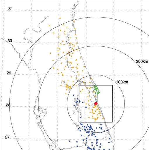
Figure 1. Map showing the locations of the MELB radar and the tipping bucket rain gauges in Florida
operated as part of the TRMM ground validation program. Also shown are the radial distance contours
of the radar FOV and the position of the 128 km area from which statistics is collected.
the asymptotic behavior of Cν(z) as z → 0 when ν < 0, we correlation c(ρ,τ) by its scaling approximation c(∞)(ρ,τ) in the
get the limit area/time integrals. The details are relegated to Appendix B.
[27] The scaling properties of the space-time covariance in
φð0; α; βÞ ¼ 2ð1þ2jνjÞ ΓðjνjÞ: (30) the β = 1 case were explored in greater detail by Kundu and
Bell [2006].
[26] Unlike the β = 1 case studied in BK96 and KB03, 2.5. Effect of a Short Distance Cut-Off
c(ρ = 0, τ) likely cannot in general be expressed in closed form. [28] As will be found later, a problem arises when we
However, scaling arguments like the one above can also be in- examine the spectral model predictions in light of the data.
voked to obtain the asymptotic τ-dependence of c(∞)(ρ = 0, τ) as We find that the growth property of the space-time covari-
1=α ance at small space-time scales in the ν < 0 case predicted
τ → 0. Setting ρ = 0 and choosing the scale factor λ ¼ τ in
equation (28), we get the asymptotic form by the spectral model is broadly consistent with data, but
only up to a certain point. The spatial variance σ 2A estimated
cð∞Þ ðρ ¼ 0; τ Þ e γ0 Kτ 2jνj=α (31) from radar data does appear to follow the predicted power
law behavior [see equation (B22)] within the accessible
range of spatial scales. But rain gauge data, which allows
as τ * → 0, where K is a dimensionless constant. This is
one to access much smaller space-time scales, exhibit a more
compatible with the general form of equation (29) if and only
complicated behavior. The scale dependence of the temporal
if φ(ξ; α, β) has the falloff
variance σ 2T follows the model prediction up to a certain
minimum averaging time T of about 30 min, but increasingly
φðξ; α; βÞ → Kξ 2jνj=α : (32) deviates from it at shorter time scales. As T → 0, instead of
ξ→ ∞
growing in accordance with the predicted power law growth,
The asymptotic behavior of the area and time-averaged σ 2T appears to gradually approach a finite asymptotic value σ 20,
statistics can be deduced by replacing the exact space-time the point variance, indicating a steeper decrease of the
10,282KUNDU AND TRAVIS: A SPECTRAL MODEL OF RAIN STATISTICS
Table 1. Model Parameters and Related Quantities for the Spectral Model
1 2 2 2 2 2
Radar Season (R) (mm h ) α β ν γ0 (mm h ) L0 (km) τ 0 (min) σ0 (mm h ) Λ (km)
KWAJ MAM 2001 0.098 0.99 1.18 0.327 0.019 281 775 2.5 0.48
KWAJ JJA 2001 0.232 0.93 1.28 0.279 0.060 438 770 7 0.36
KWAJ SON 2001 0.357 0.99 1.24 0.265 0.213 136 381 13 0.27
KWAJ DJF 2002 0.114 1.40 1.00 0.298 0.067 72.1 524 3.5 0.32
MELB DJF 2001 0.028 1.17 1.18 0.202 0.030 69.0 196 1.2 0.07
MELB MAM 2001 0.104 1.17 1.26 0.113 0.348 73.2 197 6 0.09
MELB JJA 2001 0.214 1.14 1.26 0.130 1.078 33.9 98.8 13 0.19
MELB SON 2001 0.183 1.12 1.20 0.218 0.337 51.5 209 10 0.18
characteristic time scale τ k than the model-predicted k α to obtain an estimate of Λ, we return to equation (19) for the
falloff at large k. On the other hand, the ν > 0 case of the point variance. Explicit evaluation of the integral with
model, which would have accounted for this effect, does equation (33) leads to the simple analytic result:
not generally fit the radar statistics. A simple way to incor-
porate the desired modification at short length and time 1 h jνj i
scales is to assume that instead of equation (6), τ k is given σ 20 ¼ γ0 jΓðνÞj 1 þ L20 =Λ2 1 : (34)
2
by the relation
The spatial cut-off Λ is easily obtained from equation (34) if a
( α=2 reasonable value of σ 20 can be estimated by extrapolation from
τ 0 1 þ k 2 L20 ; k < 1=Λ the gauge data.
τk ¼ (33)
0 ; k > 1=Λ
3. Comparison Between the Model
where Λ is a short distance (“ultraviolet”) cut-off. Physically and Observations
this means that the spatial Fourier modes of the precipitation
field aðk; t Þ of wavelength shorter than 2πΛ are damped out 3.1. Radar Data Analysis
instantly. Accordingly, the spectrum S(k, ω) and its tempo- [29] The parameters of the model can be conveniently esti-
ral Fourier transform c(k,τ) also vanish for wave numbers mated from a gridded radar precipitation data set. We have fit
k > 1/Λ. In a more realistic model that describes the small- the model to the data sets (TRMM standard product 2A-53)
scale behavior of rain, the sharp cut-off introduced in constructed from radar images collected from the KWAJ and
equation (33) may have to be appropriately modified based MELB radars located respectively at (8.718°N, 167.733°E)
on empirical evidence. The possibility of a steep decrease and (28.113°N, 80.654°W) (Figure 1). Next we summarize
of the spectrum beyond the scaling regime is reminiscent some relevant features of these data sets.
of a similar phenomenon in fluid turbulence, namely break- [30] For both the KWAJ and MELB radars, the FOV con-
down of the famous Kolmogorov scaling of the energy sists of a circular area of diameter 300 km. The data was
spectrum beyond the inertial range [Frisch, 1995]. In order gridded at a 2 km × 2 km spatial resolution. In order to reduce
Figure 2. Plot of the variance of area average rain rate σ2A ≡ σ2(L) as a function of the spatial
averaging scale L estimated from (left) the Melbourne radar data for the four seasons Winter
(December 2000–February 2001), Spring (March–May 2001), Summer (June–August 2001), and
Autumn (September–November 2001) and from (right) the KWAJ radar for the four seasons
Spring (March–May 2001), Summer (June–August 2001) and Autumn (September–November 2001),
and Winter (December 2001–February 2002) superimposed on the curves predicted from the model
formula (B7) with the parameters listed in Table 1.
10,283KUNDU AND TRAVIS: A SPECTRAL MODEL OF RAIN STATISTICS
Figure 3. Comparison of the spatial correlations of 2 km radar pixels as a function of the separation s as
estimated from the Melbourne radar data (the + symbols) and the spectral model (the solid curve) with the
parameters listed in Table 1 for four seasons spanning the period December 2000 to November 2001 as in
Figure 2.
the uncertainties in rain retrieval due to radar attenuation with pairs of L = 2 km radar pixels. For simplicity the measured
distance, statistics were computed from a 128 km × 128 km spatial correlation function is regarded as a function of the
area centered at the radar location by aggregating the data separation s = |s| in accordance with our spatial isotropy as-
at spatial scales L = 2, 4, 8, … , 128 km. Only those grid sumption. Since all the available pairs within the 128 km area
boxes within the selected area that had at least 95% valid are included in the computation of ΦAA′ ðsÞ, our data analysis
pixels were included in the sample. This helped eliminate automatically averages over all pair locations within the box
boxes at the smaller scales 4, 8, and 16 km located near the and allows us to assume spatial homogeneity. The direction
center, which occasionally suffered from data dropout be- dependence was implicitly averaged over two mutually per-
cause of ground clutter. pendicular directions in this step by pooling together all pairs
[31] The temporal sampling pattern of the radar has an im- with the same separation s.
portant effect on the estimation of rain statistics. The MELB [33] One effect of the uneven temporal sampling of different
radar scans were carried out at different speeds during the portions of a data set like that of the MELB radar is that it in-
quiet and the active periods of rainfall. Rainfall images were troduces a systematic bias into the usual estimates of many sta-
available from it every 5 min during the active periods and ev- tistics. In particular, the “simple” estimates of the elementary
ery 10 min during the quiet periods. Images from the KWAJ statistics at a spatial scale L, such as the unconditional mean
radar, which was operated at a single speed, are spaced in ⟨R⟩ and the probability of nonzero rain p(L) = Pr[rA > 0]
a somewhat more irregular manner: the temporal spacing obtained by summing the corresponding data and dividing
between the consecutive images predominantly alternated by the actual number of samples N(L), are biased high. One
between 5 and 7 min long gaps. can obtain “improved” estimates of these statistics that reduce
[32] The various space-time statistics of the TRMM 2A-53 this bias as follows. We assume that the temporal spacing
data needed for the analysis (the variance and covariance between two successive images Δt2 during a quiet period
functions) were computed using routines provided in the R (labeled 2), which is mostly dry, is larger than the spacing
statistical software package. For the spatial analysis we com- Δt1 during an active period (labeled 1) when rain occurs more
puted the variances σ 2A for various box sizes L between 2 and frequently. Suppose Δt2 = wΔt1; in the case of the MELB
128 km and the spatial autocorrelation function ΦAA′ ðsÞ for radar, w = 2. For each stretch of the time series of radar images
10,284KUNDU AND TRAVIS: A SPECTRAL MODEL OF RAIN STATISTICS
Figure 4. Same as in Figure 3 but for the KWAJ radar data (the + symbols) and the spectral model (the
solid curve) for the four seasons spanning the period March 2001 to February 2002.
during a quiet period, we augment it by padding each gap [35] The lagged autocorrelation ΦAA(τ) was computed for
successively with a segment consisting of (w 1) additional several averaging scales L between 2 and 128 km and for var-
copies of the initial point spaced so that the new series has a ious lags τ from the sequence of radar images. As expected, it
constant time step Δt1. was found that observed autocorrelation in general exhibits
[34] We can get a rough estimate of the bias from uneven fluctuation due to sampling uncertainty, which becomes large
sampling in the following way. Let us write N = N1 + N2, especially at those τ values where one has relatively few sam-
where N1 and N2 are the actual number of samples during ples. For our purpose, however, only those lags for which
the active and the quiet periods, respectively. For the nonzero the sampling error is small enough to be negligible were
rain probability p, instead of the naive estimate considered. In order to reduce the effect of the sampling er-
ror, we had to restrict ourselves to lags for which the number
N r>0 þ N 2r>0 of available samples exceeds a judiciously chosen value.
p¼ 1
; (35)
N1 þ N2 The estimates at the smaller scales L = 2, 4, 8,…, 64 km were
we now have the adjusted estimate obtained by partitioning the 128 km area into nonoverlapping
subareas of size L × L and averaging over the computed lagged
N r>0 þ wN r>0 autocorrelation for each subarea. Pooling together samples of
p′ ¼ 1 2
¼ Np þ ðw 1ÞN 2r>0 =N ′ ; (36) area-pairs for a fixed lag τ for the temporal autocovariance also
N 1 þ wN 2
presumes temporal stationarity of the statistics.
where N r>0
1 and N r>0
2 are the number of rainy samples during
the active and quiet periods, respectively, and N′ = N1 + wN2 3.2. Fitting the Model to Radar Rainfall Statistics
is the total number of samples in the augmented series. If [36] Estimation of the model parameters presented a diffi-
the number of rainy samples occurring during the quiet cult problem even in the simpler β = 1 case considered in
′
2KUNDU AND TRAVIS: A SPECTRAL MODEL OF RAIN STATISTICS
Figure 5. Comparison of the lagged autocorrelation at four different spatial scales (L = 2, 8, 32, and
128 km) as a function of the separation s as estimated from the MELB radar data (the symbols) and the
spectral model (the solid curve) with the parameters listed in Table 1 for the same period as in Figure 3.
However, as was noted in BK96, this approach has the disad- dependence of Φpix ðsÞ expected from the model at small sep-
vantage that the spectral estimates often suffer from distor- arations is neglected. From the gridded radar images, we first
tions at spatial scales comparable to the size of the area compute the (Pearson) sample correlation coefficients ρm for
considered (L = 128 km in our case) that are artifacts of the all pairs of pixels with spatial separation vectors sm of length
periodic boundary condition imposed by the analysis method- sm (m = 1, 2, … , M) as the estimate of the theoretical spatial
ology. This is an important issue for us since an intended appli- correlation Φpix ðsm Þ for a set of M = 66 selected values of sm
cation of the model is to perform a statistical intercomparison ranging from the minimum value of 2 km up to about 160 km
of rain rate data from ground radar and a rain gauge network (slightly less than the length of the diagonal of a 128 km box).
located within the radar FOV. While there are smoothing tech- The vectors sm are chosen so that all directions are more or
niques for the numerically evaluated spectrum that reduce less uniformly represented and there are a substantial number
these distortions somewhat [Jenkins and Watts, 1968], it is (in the range 200–23,000) of pairs Nm. We then seek to obtain
not clear to what extent the choice of a particular smoothing estimates of ν and L0 by minimizing the quantity
prescription would affect our results. Moreover, the radar data
was not uniformly spaced in time, which would therefore ne- 2
J ðν; L0 Þ ¼ ∑m¼1 wm ρm Φpix ðsm Þ ;
M
cessitate further interpolation. To circumvent these difficulties (37)
we choose to follow the approach adopted in BK96 and deter-
mine the parameters by directly fitting the statistics of the area where wm are a set of weights inversely proportional to the
averages to the model predictions. Our fitting process is in variances Σm2 of the sample spatial correlation ρm. If the sam-
effect suitably weighted so that the model faithfully represents ples entering into the computation of ρm are independent, then
the observed statistics at spatiotemporal scales of interest to us. Σm2 ∝ 1/Nm and consequently the weights are expected to be
[37] Our parameter estimation method takes advantage of proportional to the number of samples, i.e., wm ∝ Nm. In real-
the mathematical structure of the model and proceeds in ity, there is data dependency caused by the space-time corre-
two stages. First, the parameters γ0, L0, and ν are estimated lation of the rain field, thus reducing the effective number of
from the spatial statistics. The parameters ν and L0 are independent samples. The overall effect of this dependency
obtained from a suitably weighted least squares fit to the spa- for our estimation problem is somewhat difficult to assess
tial correlation function Φpix ðsÞ ≡ ΦAA′ ðsÞ for 2 km pixels sep- and will not be taken into consideration here. Evaluation of
arated by a distance s = |s|. For simplicity, the slight direction the model spatial correlations Φpix ðsm Þ is carried out from
10,286KUNDU AND TRAVIS: A SPECTRAL MODEL OF RAIN STATISTICS
Figure 6. Same as in Figure 5 but for the KWAJ radar data (the symbols) and the spectral model (the solid
curve) for the same period as in Figure 4.
equation (B5) using the software Mathematica, version 9, up to a certain reasonably large τ. Values of β and τ 0 are
from Wolfram, Inc. The minimum of J(ν, L0) is sought by estimated by minimizing the quantity
employing the numerical implementation of the Nelder-
h i 2
Mead Simplex Algorithm [Nelder and Mead, 1965; Press J^ ðβ; τ 0 Þ ¼ ∑j¼1 w
n
^ j ρ^j ΦAA τ j (38)
et al, 1992; Lagarias et al, 1998] in Mathematica. A starting
value for the index ν can be obtained by fitting the asymp-
totic form equation (B22) to the variance σ 2A for small L. using the Nelder-Mead Simplex Algorithm in Mathematica.
The computation of the spatial parameters ν and L0 for each The weights w ^ j can now be taken to be 1 (the ordinary least
data set was quite efficient and took only a few minutes on squares case) since the numbers of samples are roughly equal
a desktop computer equipped with two Quad-core Intel for all lags in the range considered. The observed lagged
Xeon processors. The normalization constant γ0 is fixed by autocorrelation was found to exhibit large systematic depar-
a least squares fit of the model prediction (using the exact for- ture from the model-predicted form for larger values of τ.
mula (B7)) to the observed variances σ 2A . The Nelder-Mead We therefore had to restrict the range of τ over which the
Algorithm, despite its heuristic nature, is our preferred choice fit was carried out (about 400 min for KWAJ and 200 min
for an optimization method primarily because of its simplic- for MELB).
ity and speed of execution. For a test run on a KWAJ radar [39] Unfortunately, evaluation of the quantities ΦAA(τ j) in-
data set, the Differential Evolution Method [Storn and volves computing (2 + 1) dimensional integrals in the Fourier
Price, 1997], a global optimization method available within space of k and ω making the optimization problem computa-
Mathematica, gave results for ν and L0 that are substantially tionally rather onerous. The Nelder-Mead Algorithm took a
identical with those from the Nelder-Mead Method but took long time to converge. The execution time depended on the
much longer (about 28 times) to converge. number of lag values employed to define the sum of squares
[38] The next step is to estimate the temporal parameters J^ ðβ; τ 0 Þ; for each data set it typically took about 1 h per value
τ 0, β (and therefore α). They can be determined by fitting of j on a workstation equipped with an Intel i7 870 processor.
the lagged autocorrelation function ΦAA(τ) for a particular We should note that in estimating these parameters, the short
box size L. We calculated the model values ΦAA(τ j) using distance cut-off parameter Λ is implicitly set to zero with the
equations (B6) and (B7) and fit them to the observed values anticipation that it is sufficiently small compared to the
ρ^j for a 16 km box and a set of time lags τ = τ j (j = 1, 2, …, n) smallest spatial scale accessible to radar measurements. Its
10,287KUNDU AND TRAVIS: A SPECTRAL MODEL OF RAIN STATISTICS
Figure 7. Plot of the variance of time-averaged point rain rate σT2 as a function of the averaging scale T
for precipitation data from the TB gauges located within the MELB radar FOV. The panels exhibit results
for the same time period December 2000 to November 2001 divided into four seasons as in Figure 2. The
open circles denote the observed variance and the solid curve represents the model results.
value can only be meaningfully estimated from the gauge constant γ0 varies widely from one data set to another and ap-
data at very short time scales. pears to be related to the mean rain rate. Figure 2 shows a
[40] We divided the 2A-53 annual radar precipitation data comparison of the variances σ 2A deduced from the data (sym-
sets from the KWAJ and MELB radars into four 3 month bols) and those computed from the model (solid curve) for
long seasons—Winter (December–February, or DJF), Spring various box sizes L. The fits to the spatial correlation function
(March–May, or MAM), Summer (June–August, or JJA) ΦAA′ ðsÞ for the L = 2 km radar pixels as a function of the sep-
and Autumn (September–November, or SON), and carried aration s are shown in Figures 3 and 4 for the MELB and
out the estimation of the model parameters for each. In doing KWAJ radars, respectively. The quality of the fits for the
so, we implicitly regard the statistics of each season as station- temporal statistics is illustrated in Figure 5 (for the MELB
ary in the wide sense. Here we present results of parameter radar) and Figure 6 (for the KWAJ radar) by the plots of
estimation for four seasons for each of these two radars. For ΦAA(τ) at several other spatial scales. It is seen that the model
the MELB radar, we selected the 2001 DJF, MAM, JJA, and fits the observation reasonably well for spatial scales L
SON seasons. For the KWAJ radar, DJF 2001 data had to be between 2 and 32 km, but the fit becomes worse at larger
excluded from the analysis because of the highly erratic behav- scales. By allowing the order of the time derivative β to be
ior of the temporal correlation, and so we considered DJF 2002 an adjustable noninteger parameter, a closer fit at small τ is
instead as a representative example. achieved for the temporal statistics compared to the β = 1 case
[41] The model parameters are listed in Table 1. The spatial of the model, as illustrated in Appendix B (Figure B2) for the
index ν lies in the range 0.27 to 0.33 for the KWAJ radar KWAJ JJA 2001 season.
and 0.11 to 0.22 for the MELB radar. The temporal index
β is found to be substantially greater than 1, in fact lying in 3.3. Validating the Model with Rain Gauge Data
the narrow range 1.2–1.3, in all cases except one, namely [42] In this section we compare the model predictions
the KWAJ DJF 2002 season. The characteristic length and for the statistics of time-averaged point rain rate outlined
time scales L0 and τ 0 are generally longer for the KWAJ data in section 2.4 with the statistics of rain gauge observa-
sets than the MELB data sets, which is presumably attribut- tions. The temporal statistics were obtained from a rain
able to the purely oceanic environment of the former. The gauge data set (TRMM standard product 2A-56) for the
10,288KUNDU AND TRAVIS: A SPECTRAL MODEL OF RAIN STATISTICS
Figure 8. Plot of the spatial correlation ΨTT(ρ) of the daily averaged gauge data as a function of the gauge
separation ρ for the same data set as in Figure 7. The panels exhibit results for the same time period
December 2000 to November 2001 divided into four seasons as in Figure 2. The + symbols denote the ob-
served correlation for each gauge pair. The open circles denote the observed correlation averaged over all
gauge pairs in each distance bin interpolated by the solid curve. The error bars are estimated according to
the method described in the text. The dashed curve represents the results computed from the model.
same time period over which the spectral model parame- separation bins. The average over each bin was estimated
ters were obtained in section 3. The data consists of as follows. A Fisher z-transform z = tanh 1Ψ, which maps
estimates of 1 min rain rate derived from rainfall accumula- the interval (1, 1) onto the real line, was applied to the cor-
tions in the tipping bucket (TB) gauges located within the relation estimates for each gauge pair. It is well-known that
same central 128 km area within the radar field-of-view [Hawkins, 1989] for a fairly large class of probability distri-
(FOV) that was used to extract the radar statistics during a butions of the correlation estimates Ψ, the variable z is nearly
particular period of observation (Figure 1). For the KWAJ normal and consequently, the standard estimates of the
radar FOV, there were only seven gauge locations, each confidence intervals apply. The inverse transform Ψ = tanh z
equipped with paired TB gauges and, moreover, not all of is then applied to the statistics obtained from the normal
them were available for every season. For the MELB radar, theory to determine the average correlation and the corre-
there were about 50–60 gauges available within the central sponding 95% confidence intervals for each separation
128 km box. bin. In practice, the histograms of the z-transformed values
[43] We computed an estimate of the observed temporal turned out to be slightly non-normal. We therefore checked
variance σ 2T for T in the range 1–7200 min by taking the the accuracy of our results by constructing a bootstrap
average over a moving window of length T for each gauge distribution from 10,000 replicas of a random sample drawn
along the time series and computing the variance for the full from the underlying empirical distribution and constructing
set of gauges for the entire season. The variances for the indi- bootstrap confidence intervals [Efron, 1981]. The resulting
vidual gauges were averaged together to estimate σ 2T . The bias of the bootstrap estimate of the mean was found to be
spatial correlation of the gauge pairs ΨTT(ρ) was also com- negligibly small and the estimated confidence intervals
puted for daily averaged rain rates (T = 1440 min). For the agreed well with the normal statistics estimates. For the
MELB data set, the average spatial correlations between KWAJ data, the gauge distribution was very sparse, and with
gauge pairs were estimated by binning them into spatial the small number of rain gauges that were available in the area,
10,289You can also read