Influence of Vaporfly shoe on sub-2 hour marathon and other top running performances
←
→
Page content transcription
If your browser does not render page correctly, please read the page content below
Influence of Vaporfly shoe on sub-2 hour marathon
                                                      and other top running performances
                                                                 Andreu Arderiu∗1 and Raphaël de Fondeville†2
                                                     1
                                                         Department of Mathematics, Ecole Polytechnique Fédérale de
                                                                                 Lausanne
arXiv:2104.08509v1 [stat.AP] 17 Apr 2021

                                                                        2
                                                                          Swiss Data Science Center

                                                                                     April 20, 2021

                                                                                         Abstract

                                                        In 2019, Eliud Chipgoke ran a sub-two hour marathon in an unofficial race
                                                     wearing last-generation shoes. The legitimacy of this feat was naturally questioned
                                                     due to unusual racing conditions and suspicions of technological doping. In this
                                                     work, we assess the likelihood of a sub-two hour marathon in an official race, and
                                                     the potential influence of Vaporfly shoes, by studying the evolution of running
                                                     top performances from 2001 to 2019 for distances ranging from 10k to marathon.
                                                     The analysis is performed using extreme value theory, a field of statistics dealing
                                                     with analysis of records. We find a significant evidence of technological doping
                                                     with a 12% increase of the probability that a new world record for marathon-
                                                     man discipline is set in 2021. However, results suggest that achieving a sub-two
                                                     hour marathon in an official event in 2021 is still very unlikely, and exceeds 10%
                                                     probability only by 2025.

                                           Keywords: Athletics performance, running time records, statistical analysis, Vaporlfly.

                                           1         Introduction
                                           In 2016, Nike released the new generation Vaporfly 4% shoes with slogan “Designed for record
                                           breaking speed”. As a part of its advertisement campaign, the brand initiated the “Breaking
                                           2” project, with the aim to break the two-hour marathon barrier. Since then, the sport
                                           community had growing suspicions that 2016-released shoes, and subsequent models, had a
                                           significant effect on running performance. The technology behind these models includes a very
                                           light and responsive foam sole combined with an embedded curved carbon fibre plate, which
                                           allegedly give an advantage to athletes wearing them. Therefore, these controversial shoes
                                           sparked a vivid debate, that was concluded by a ban in January 2020 from world athletic
                                               ∗
                                                   andreu.arderiu@epfl.ch
                                               †
                                                   raphael.de-fondeville@epfl.ch

                                                                                             1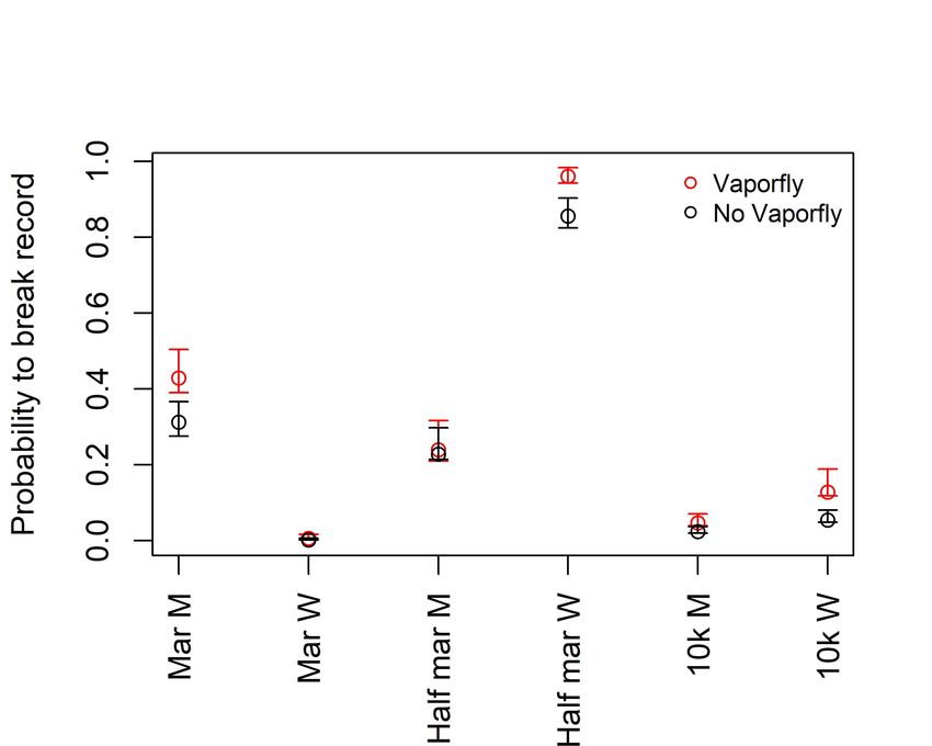
official races. This situation is reminiscent of the 2010 ban in elite swimming of Speedo’s
record-breaking full body swimsuit.
Several study attempted to quantify the influence of Nike’s technology on running performance:
Hoogkamer et al. (2018) conducted laboratory experiments with professional runners and
found that Vaporfly’s reduced the energetic cost by an average of 4%, giving its name to
the first model. Later, Hoogkamer et al. (2019), and Barnes and Kilding (2019), monitored
biomechanical and physiological variables to assess the effect of carbon fibre new generation
shoes on long distance runners. They confirmed the presence of a 4% energy reduction in
average compared to other popular racing shoes. In parallel, Wired Magazine (Thomson,
2017) performed simple data analysis on running times achieved during the New York City
Marathon by amateurs wearing Vaporfly shoes and found that, on average, they ran the
second half of the race faster than other participants. Similarly, in a subsequent analysis,
Quealy and Katz, 2019 found that Vaporfly users ran from 2% to 5% faster in marathons and
half marathons. Recently, Guinness et al. (2020) compared marathon running-times of elite
runners, with and without Vaporfly shoes, and estimated a performance increase of 1% to 4%.
All these works focused on the impact of Vaporfly shoes on average performances, and so far
as we know, no such analysis has been performed on fastest times. We thus propose to study
fastest running times over the past few years, which we model as rare extreme events, i.e., large
deviations from average running times. Extreme-value theory (EVT) is a branch of statistics
that specifically deals with such extremes and that has been successfully applied to analyse Ath-
letics performances in various context: Strand and Boes (1998) analysed the relation between
age and performance for 10k road race athletes, and estimated their age of peak performance.
Blest (1996) analysed historical world records for various athletic disciplines to assess the exis-
tence of best achievable performances. Robinson and Tawn (1995) analysed women’s 1500 and
3000m running times to estimate the best achievable performance for woman’s 3000m track,
and assess if a recently broken record was susceptible to be achieved under drug enhancement.
Later, Stephenson and Tawn (2013), used data from different Olympic disciplines, both for
man and woman, to compare the history of world records across disciplines. In a different
fashion, J. H. J. Einmahl et al. (2008) and Rodrigues et al. (2011) compared the quality of
world records for different disciplines by estimating their best achievable performance.
In our study, we aim to quantify the influence of Vaporfly shoes on fastest times, i.e., assessing
their impact on the frequency that a distance is ran under a given time in a given year, and
on the corresponding running times. We propose a statistical model allowing to estimate the
probability that a sub 2 hour marathon is run in a given year while accounting for potential
technological doping by Vaporfly shoes. In this regard, similarly as Spearing et al. (2021)
did for elite swimmers data, we leverage extreme value theory to compare the effect of new
generation shoes across genders and distances, while accounting for the constant improvement
over time of running techniques and training practices.
The paper proceeds as follows. Section 2 gives a detailed description of the data, as well as the
methodology applied in our study. In Section 3, we present our main conclusions, including
expected next records, the likelihood of a sub-two hour marathon, the probability of breaking
world records, and running-times adjusted to correct for the Vaporfly effect. We report a
significant evidence of technological doping, with Vaporfly shoes accounting for a 12% increase
of the probability that a new world record for marathon-man discipline is set in 2021. However,
results suggest that achieving a sub-two hour marathon in an official event in 2021 is still very
unlikely, and exceeds 10% probability only by 2025. Finally, Section 4 concludes by discussing

                                                2
some limitations of our model, and suggests directions for further improvements.
2 Methodolgy
2.1 Data Exploration
In this study, we extract yearly top-100 running-times, in seconds, over the period 2001 to
2019 for marathon, half-marathon and 10k road disciplines; only official events as labelled by
World Athletics are considered. As it is commonly done in sports data analysis, we consider
man and woman data as different disciplines yielding a total of six disciplines with 1900 data
points each.
Our aim is to estimate the probability that a running time drops below a given reference. In this
setting, best performances correspond to the shortest race times, and we focus on extremely
low running times, that can be viewed as large negative deviations from the average. A
natural tool to analyse such extreme events is Extreme Value Theory, and in particular Peaks-
over-Threshold (POT) analysis: the methodology provides a framework to approximate the
distribution of exceedances, i.e., the probability, and its frequency, that a variable drops below
a given threshold. In practice, we simply fit a statistical model to any data point that exceeds
a large negative threshold.
The mathematical formulation of the model is theoretically justified as it corresponds to the
universal approximator of the distribution of independent exceedances. For this reason, the
model can be used for extrapolation, i.e., quantify the probability of running times that have
not been observed yet. An important parameter, the tail index, determines the regime of
extrapolation: a positive tail index implies that any running time below the threshold has
a positive probability of occurrence; while for a negative tail indexes observations are lower
bounded. In sports, multiple studies, e.g., Robinson and Tawn, 1995; Blest, 1996; Strand
and Boes, 1998; J. H. J. Einmahl and Magnus, 2008; Rodrigues et al., 2011, found negative
indexes giving strong evidences in favor of the existence of a best achievable performance.
Similar analysis have also been performed in other context such as life expectancy (J. J.
Einmahl et al., 2019), natural hazards (Holmes et al., 2008) or hydrology (Katz et al., 2002).
Throughout this article, we assume independence between all running-times across distances,
years, and disciplines, even if some records were set by the same athlete.
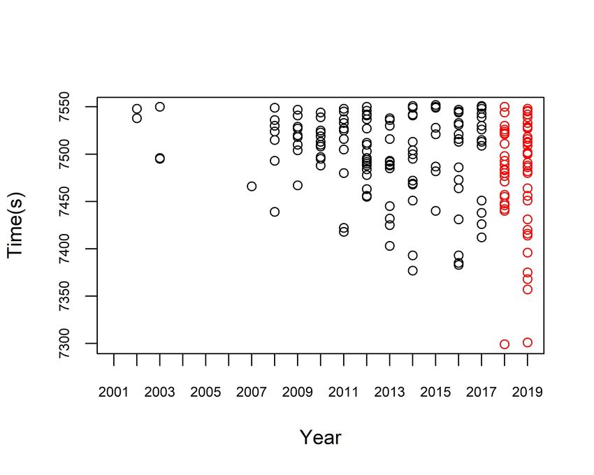
For each discipline, we select a threshold such that over the period 2001 to 2019 there are
exactly 200 runing-times that drop below; data for the man’s marathon is displayed in Figure
1. We observe a temporal increase in both race time performance, and frequency at which
exceedances occur. We also note a noticeable step increase in year 2018 and 2019, correspond-
ing to the democratization of Vaporfly shoes amongst elite runners (Quealy and Katz, 2019).
The unexpected and sudden frequency increase in 2012 mostly roots by an exceptionally fast
marathon in Abu Dhabi that year. Similar trends are observed across all disciplines.
3
Fig. 1: Man’s marathon best running times from 2001 to 2019. Left: 200 best all-time
marathon running-times per year. Right: yearly number of running times within a given
year. Red points (bars) correspond to observations (years) for which Vaporfly shoes are
widely used in official races.

2.2     Model
For each discipline, we model running times dropping below their respective thresholds fol-
lowing the work of Spearing et al. (2021) for Elite Swimmers; technical methodological details
can be found in Appendix A. The model provides estimates for the expected number of ex-
ceedances per year, as well as the probability that the running time falls below given lower
references. Furthermore, as we find negative tail indexes for every discipline, the model pro-
vides an estimate for the lowest achievable running time within a year that we call ultimate
time.
The model includes time-dependent parameters to account for the improvements of racing and
athletes conditions over time, as well as for a ”Vaporfly effect” which we assume to appear in
2018, when the shoes started to be widely used in official races. Multiple models with different
temporal dependencies were considered, but none of them were significantly better than the
presented model. Parameter estimates retrieve for all disciplines a positive temporal trend for
improvements in running techniques and training practices, which is specially significant for
marathon-man and half marathon-woman. Similarly, the Vaporfly effect is found significant
and positive across all disciplines, clearly indicating the presence of some technological doping.
The impact is stronger for woman than for man: for instance, the effect is 200% stronger for
marathon-woman than for marathon-man.
To assess the overall quality of the fitted model, we compared yearly frequencies and running
times faster than their respective threshold, to the theoretical quantities provided by the fitted
model; see Appendix C. The fit is overall good.

                                                4
3     Results
3.1     Yearly ultimate times
We computed the ultimate times for all six disciplines as function of time: these change
linearly with time accounting for continuous improvement of techniques and preparation over
time. Table 1 displays the world records as in 2019 for all disciplines against ultimate times
for 2019 and 2025: we observe a substantial decrease for marathon-man from 2019 to 2025.
In contrast, the ultimate time for marathon-woman just decreases few seconds over the same
period. To our knowledge, there is no obvious explanation for such variability of the rate of
change across disciplines.

Table 1: World records as in 2019 and ultimate times for 2019 and 2025, for all
disciplines, with 95% confidence intervals.

       discipline    World record 2019                  Ultimate 2019            Ultimate 2025
    Marathon-man         02:01:39                    01:59:44 (-20s,+16s)     01:58:07 (-23s,+18s)
   Marathon-woman        02:14:04                    02:13:01 (-44s,+16s)     02:12:54 (-47s,+17s)
  Half marathon-man      00:58:01                     00:57:21 (-7s,+6s)       00:56:58 (-7s,+7s)
 Half marathon-woman     01:04:51                    01:02:26 (-17s,+16s)     01:01:23 (-19s,+19s)
       10k-man           00:26:38                     00:26:20 (-5s,+4s)       00:26:13 (-5s,+5s)
      10k-woman          00:29:43                     00:29:09 (-10s,+4s)     00:28:59 (-10s,+5s)

3.2     Expected next record
The model provides the probability that a running time drops below given reference times. We
can thus set the reference to the current world record, and estimate the expected running-time
of a new record in a given year. Figure 2 displays the estimated expected running-time of the
next world record for the year 2021 with corresponding ultimate times. Different disciplines
have different scales of time so, to ensure a proper comparison between disciplines, we scale all
values by their respective 2019 world records. As an example, the marathon-man 2019 world
record is 2h 1m 39s, and the 2021 ultimate time is 1h 59m 11s, so their ratio in seconds is
0.98. The difference between expected new world record and ultimate times gives an idea of
how close we expect the new record to be to the fastest possible time in 2021.
In Figure 2, differences between expected new record and ultimate running time vary across
different disciplines, ranging from 53s, i.e., 0.8%, for marathon-woman, to 2m 14s, i.e., 4.3%, for
half marathon-woman. Expected improvements of world records in 2021 are slightly smaller
in percentage for disciplines where the current record is closer to the fastest possible time,
but differences are relatively small ranging from 0.2% for marathon-woman to 0.8% for half
marathon-woman, which stems from the common tail index shared across disciplines. As the
ultimate time decreases over time, if the record is not broken then the gap between current
record and ultimate time increases, giving range for greater improvement.

                                                5
Fig. 2: Expected (black) new world records, if it were to be broken in 2021, and
corresponding ultimate times (red) for every discipline, with 95% confidence intervals.
For clarity, estimated times are normalised by the current record as of 2019.
                                           .

3.3    Probability of record breaking in a given year
We can use the fitted model to estimate the probabilities of breaking a world record in any
given year after 2019. Figure 3 displays the estimated probabilities of breaking the world
record in 2021 with and without correcting for the effect of Vaporfly shoes.
We observe how probabilities vary significantly from discipline to discipline, ranging from a
1% chance for marathon-woman to a 96% chance for half marathon-woman. Such low chance
for marathon-woman is coherent with the fact that the difference between its current world
record and 2021 ultimate time is the smallest across disciplines, so its record might be harder
to break than for other disciplines. Estimates correcting for the effect of Vaporfly shoes are
extremely similar for marathon-woman, half marathon-man, and 10k-man, which contrasts
with the substantial probability drop of about 12%, 10%, and 8% for marathon-man, half
marathon-woman, and 10k-woman disciplines, respectively.

                                              6
Fig. 3: Probability of the world record being broken in 2021 for all disciplines, with 95%
confidence intervals. Red dots: estimates with Vaporfly shoes. Black dots: corrected
estimates removing the effect of Vaporfly shoes.
                                           .

3.4     Time until next record breaking
In the previous section we estimated the probability of breaking a record in a given year. In a
similar fashion, we can use the fitted model to estimate the probability of the current record
to be broken before a given year. These are computed for consecutive years, and we find
for each discipline the earliest year for which such probability exceeds 95%. In other words,
we estimate the expected maximum waiting time to observe a new record, with at least 95%
certainty; results are displayed in Table 2 with and without Vaporfly adjustment.
It is remarkable that for marathon-man the world record will most likely be broken before 2025.
At first glance it might be surprising that when correcting for the Vaporfly effect, the estimated
year is increased by just one year for marathon-man, when the probability of breaking record
in 2021 was dropping by a 12%. This is the consequence of a substantial yearly increase of
the probability to break the world record for this discipline, reaching values close to 1 in few
years, even when neglecting the shoes effect. Conversely, for disciplines where the estimated
year is greater, as for marathon-woman, the increase due to the Vaporfly effect is much more
substantial.

                                                7
Table 2: Estimated earliest year before which there are 95% chances that the current
world record is broken, with 95% confidence intervals. Vaporfly years correspond to
estimates with Vaporfly shoes authorized, while the rightmost column correspond to
the estimates corrected to remove the influence of the shoes.

                 discipline           Year Vaporfly Year Vaporfly-corrected
              Marathon-man            2025 (-1y,+0y)    2026 (-1y,+0y)
             Marathon-woman           2043 (-2y,+1y)    2051 (-3y,+0y)
            Half marathon-man         2026 (-0y,+1y)    2027 (-1y,+0y)
           Half marathon-woman        2022 (-1y,+0y)    2022 (-0y,+0y)
                 10k-man              2036 (-1y,+1y)    2041 (-2y,+0y)
                10k-woman             2030 (-1y,+1y)    2035 (-1y,+1y)

Similarly, we can further estimate the expected waiting time until the current world record is
broken for each discipline. Table 3 shows the estimates for the expected waiting times, and
their corrections obtained by removing the Vaporfly effect. We observe for marathon-man that
the current world record is expected to be broken in 2 years, which contrasts with marathon-
woman, where the expected waiting time is 16 years. For the rest of disciplines, it can be seen
that expected waiting times are below 10 years. It is also remarkable that when neglecting the
Vaporfly effect, waiting times substantially increase for all disciplines but marathon-man, half
marathon-man and half marathon-woman. This is coherent with the previous analysis made
for Table 2.

Table 3: Expected waiting time, in years with 95% confidence intervals, until next
record is set for all disciplines. Vaporfly times correspond to estimates with Vaporfly
shoes authorized, whereas the rightmost column correspond to times corrected to remove
the Vaporfly effect.

                discipline    Time Vaporfly Time Vaporfly-corrected
             Marathon-man      2.3 (2.1,2.5)     2.9 (2.6,3.0)
            Marathon-woman    16.6 (12.8,17.0) 23.0 (18.7,23.7)
           Half marathon-man   3.3 (2.9,3.6)     3.4 (3.1,3.6)
          Half marathon-woman  1.1 (1.1,1.1)     1.3 (1.2,1.3)
                10k-man        8.7 (7.3,9.1)   11.7 (10.1,12.3)
               10k-woman       5.2 (4.1,5.6)     8.2 (6.9,8.8)

3.5    Corrected times without the Vaporfly effect
In a similar fashion as Spearing et al. (2019) did for the use of full body suits in swimming,
we can adjust running-times for the use of the Vaporfly shoes. More precisely, for a given
discipline, the corrected running-time of a performance achieved during the Vaporfly period
2018-2019 is computed by matching probabilities of exceedances with and without the Vaporfly
effect.
As an example, the current world record for marathon-woman is 2 hour 14 minutes and 4
seconds, which was set in 2019 by Brigid Kosgei wearing Vaporfly shoes. If we adjust such

                                               8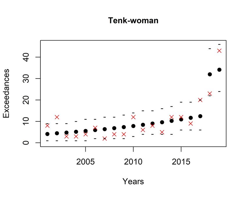
record time for the Vaporfly effect, we obtain 2 hour 16 minutes and 3 seconds, which represents
a correction of +119 seconds. This suggests that if Vaporfly shoes hadn’t been used in 2019,
the world record would still be the 2 hour 15 minutes 25 seconds, set by Paula Radcliffe in
2010.

3.6     Likelihood of a sub-two hour marathon
The two-hour marathon barrier had been long since regarded as unbreakable. In 2016 within
the project Breaking 2, Nike organised a race during which Eliud Kipchoge set a time of 2 hours
and 25 seconds. In 2019, Ineos organised the 1:59 Challenge race, where Eliud successfully
broke the barrier, achieving a time of 1 hour 59 minutes 40 seconds. However, neither of those
records are officially recognised, as race conditions were controlled and a rotating cast of pacers
shielded him from wind throughout the run. Indeed, in Table 1 the estimate for the ultimate
or fastest possible running-time of marathon-man in 2019 is of 1 hour 59 minutes 44 seconds,
which suggests that even though a sub-two hour marathon would have been theoretically
possible, the time achieved by Kipchoge in the Ineos challenge would have been very unlikely
with regular official race conditions.
Some study attempted to predict the year when the first sub two-hour marathon would be
achieved: Joyner et al. (2011) estimated the rate of improvement of marathon-man world
records since the late 1920s, finding that a time under 2h could occur between 2021 and 2036.
Angus (2019) used marathon world record performance times since 1950, and estimated that
the probability of observing a sub-two hour marathon in 2020 is just about 3%, with chances
increasing to 10% by 2032.
The estimated probability of a sub-two hour marathon in 2020 obtained with our model is of
0.1% (0.04%, 0.3%), much lower than the estimate provided by Angus. Such discrepancy can
be explained by the fact that, while we base our analysis on 200 top times for each discipline,
Angus just use world record progression data with a total of 26 data points, so their estimates
might suffer from high variability. Still, both results agree that it is still very unlikely that
without controlling race conditions or offering additional support for runners a sub two-hour
marathon can be achieved in 2020.
Additionally, we compute estimates for the probability that a sub two-hour marathon is
achieved in a given year. Figure 4 (left) displays such estimates for the 2020-2030 period,
with and without the Vaporfly technology. We observe how before 2025 all probabilities are
below 10%, and the chances of breaking the two hour barrier with and without the Vaporfly
effect aren’t significantly different. Note also that 2030 is the first year where the chances
of breaking the barrier exceeds 50%. In that case, if we neglect shoes effect, chances fall to
around 40%. Figure 4 (right) displays cumulative probability estimates, so the chances that a
sub two-hour marathon is achieved before a given year. We observe that there are about 10%
and 50% chances that a sub two-hour marathon is achieved before year 2025 and year 2029,
respectively.

                                                9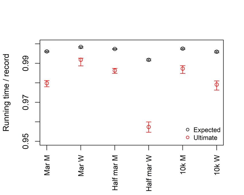
Fig. 4: Probability that the a sub two-hour marathon is achieved by a man in a given
year (left), and before a given year (right), for the 2020-2030 period with 95% confidence
intervals. Red dots correspond to the probability computed with Vaporfly technology,
whereas black dots are corrected for such technological doping.

Finally, the expected sub two-hour marathon arrival time is found to be 2027, which is coherent
with the 2021-2036 range estimated by Joyner et al. in 2011.

4     Discussion
The main purpose of this study was to analyse the evolution of the frequency and distribution
of top running times from various running disciplines, and assess the possible influence of
Vaporfly shoes usage. Our results suggest that performance substantially improved over time
for all disciplines due to the improvements in running techniques and training practices, and
that Vaporfly shoes influence is significant, with greater impact for woman than for man.
Furthermore, we showed how in some cases the Vaporfly effect could question current world
records, e.g., marathon-woman. Moreover, our results showed that it is still very unlikely that
a sub-two hour marathon is achieved in an official race during the next few years, and that
the record achieved by Chipgoke in Ineos Challenge would have been very unlikely without all
the additional support and controlled racing conditions.
The model has a good overall fit, and provides a good agreement with historical records.
However, we couldn’t fully explain the variability of some model parameters, such as the
linear trends, across different disciplines. One of the underlying assumptions of our model
is that the number of official races held for every discipline doesn’t substantially change,
so observations for every year are equally weighted. Hence, we might be over-, or under-,
weighting observations from years where more, or less, races were held; the year 2020, excluded
of this analysis, would be an obvious example. Such yearly data imbalance could be taken
into account for more accurate estimation and forecasting. Furthermore, we didn’t account for
the different race conditions of the venues, which certainly have an impact in the distribution

                                              10
of times. In this aspect, the model could be improved by adding an additional parameter for
each venue to capture their influence in running-times. Finally, we assumed that before 2018
there were no times recorded with Vaporfly shoes, and after 2018 times were set with such
shoes. To improve our model estimation of the influence of such shoes, it could be relevant to
label each data points as performed with or without the shoes, similarly as in Guinness et al.
(2020).
Acknowledgement
We acknowledge Harry Spearing for sharing code that provided good inspiration to our work.The
authors received no specific funding for this work.
Disclosure of interest
The authors report no conflict of interest.
References
Angus, S. D. (2019). A statistical timetable for the sub–2-hour marathon. Medicine &
Science in Sports & Exercise, 51 (7), 1460–1466.
Barnes, K. R., & Kilding, A. E. (2019). A randomized crossover study investigating the
running economy of highly-trained male and female distance runners in marathon
racing shoes versus track spikes. Sports Medicine, 49 (2), 331–342.
Blest, D. C. (1996). Lower bounds for athletic performance. Journal of the Royal Sta-
tistical Society. Series D (The Statistician), 45 (2), 243–253.
Coles, S. (2001). An introduction to statistical modeling of extreme values. Springer.
Davison, A. C., & Smith, R. L. (1990). Models for exceedances over high thresholds.
Journal of the Royal Statistical Society. Series B (Methodological), 52 (3), 393–
425.
Einmahl, J. J., Einmahl, J. H. J., & Haan, L. d. (2019). Limits to human life span
through extreme value theory. Journal of the American Statistical Association,
114 (527), 1075–1080.
Einmahl, J. H. J., & Magnus, J. R. (2008). Records in athletics through extreme-value
theory. Journal of the American Statistical Association, 103 (484), 1382–1391.
Guinness, J., Bhattacharya, D., Chen, J., Chen, M., & Loh, A. (2020). An obser-
vational study of the effect of nike vaporfly shoes on marathon performance.
arXiv:2002.06105 [stat].
Gumbel, E. J. (1958). Statistics of extremes. Columbia University Press.
Holmes, T., Huggett, R., & Westerling, A. (2008). Statistical analysis of large wild-
fires. The economics of forest disturbances: Wildfires, storms, and invasive species
(pp. 59–77). Springer, Dordrecht.
Hoogkamer, W., Kipp, S., Frank, J. H., Farina, E. M., Luo, G., & Kram, R. (2018).
A comparison of the energetic cost of running in marathon racing shoes. Sports
Medicine, 48 (4), 1009–1019.
11Hoogkamer, W., Kipp, S., & Kram, R. (2019). The biomechanics of competitive male
runners in three marathon racing shoes: A randomized crossover study. Sports
Medicine, 49 (1), 133–143.
Joyner, M. J., Ruiz, J. R., & Lucia, A. (2011). The two-hour marathon: Who and when?
Journal of Applied Physiology, 110 (1), 275–277.
Katz, R. W., Parlange, M. B., & Naveau, P. (2002). Statistics of extremes in hydrology.
Advances in Water Resources, 25 (8), 1287–1304.
Quealy, K., & Katz, J. (2019, December 13). Nike’s fastest shoes may give runners an
even bigger advantage than we thought. https://www.nytimes.com/interactive/
2019/12/13/upshot/nike-vaporfly-next-percent-shoe-estimates.html
Robinson, M. E., & Tawn, J. A. (1995). Statistics for exceptional athletics records.
Journal of the Royal Statistical Society. Series C (Applied Statistics), 44 (4),
499–511.
Rodrigues, L., Gomes, M., & Pestana, D. (2011). Statistics of extremes in athletics.
Revstat Statistical Journal, 9 (2), 127–153.
Scarrott, C., & MacDonald, A. (2012). A review of extreme value threshold estimation
and uncertainty quantification. Revstat Statistical Journal, 10 (1), 33–60.
Spearing, H., Tawn, J., Irons, D., Paulden, T., & Bennett, G. (2021). Ranking, and
other properties, of elite swimmers using extreme value theory. Journal of the
Royal Statistical Society: Series A (Statistics in Society), 184 (1), 368–395.
Stephenson, A., & Tawn, J. (2013). Determining the best track performances of all time
using a conceptual population model for athletics records. Journal of Quantitative
Analysis in Sports, 9 (1), 67–76.
Strand, M., & Boes, D. (1998). Modeling road racing times of competitive recreational
runners using extreme value theory. The American Statistician, 52 (3), 205–210.
Thomson, N. (2017, July 11). Do nike’s zoom vaporfly 4% marathon shoes actually
make you run faster? — WIRED. https://www.wired.com/story/do-nike-zoom-
vaporfly-make-you-run-faster/
12Appendices
A Theory and Model
A.1 Extremes for identically distributed variables
Extreme value theory (EVT) is a branch of statistics which study the tails of probability
distributions. It was first developed for block maxima (Gumbel, 1958) analysis, but the Peaks
Over Threshold (POT) method (Davison and Smith, 1990) is often preferred, as it uses all the
most extreme data, rather than just the maxima, typically leading to more efficient inference.
Let X be a random variable with distribution function F , if there exist random sequences an ,
bn > 0 such that
n {(1 − F (an x + bn )} −→ − log G(x) (A.1)
as n −→ ∞ is a non-degenerate limiting distribution, then for a large enough threshold u we
can use the approximation
(
1 − [1 + ξ{(x − u)/σu }]−1/ξ ξ 6= 0,
P r(X > x|X > u) ≈ Hu (x) = x ∈ R, (A.2)
1 − exp{−(x − µ)/σu }, ξ = 0,
where σu = σ + ξ(u − µ) > 0, a+ = max(a, 0). If ξ < 0 then x must lie in the interval [0, xH ],
where xH = u − σu /ξ is the upper limit of the distribution, whereas if ξ ≥ 0, x can take
any positive value. The limit distribution Hu , called Generalized Pareto distribution (GPD)
motivates an approximation for large u, giving a model for the distribution of the exceedances
above such threshold, regardless of the distribution F .
Given a large enough sample of n independent identically distributed (IID) observations, in the
POT approach a threshold u is carefully chosen, and exceedances can be used to estimate the
parameters of the GPD. Threshold choice can be rather subjective and case-dependent, and is
subject to a bias-variance trade-off. In this paper we base our choice on graphical diagnostics;
however, other alternative methods might also be suitable; see Scarrott and MacDonald (2012)
for a detailed review of these techniques.
It is remarkable that the rate of the frequency of exceedances above the threshold u can be
derived in a fashion that gives way to a more complete perspective of exceedances modelling,
using point process models. Let Xi be IID random variables with distribution function F , we
define
n
1(Xi > an x + bn ),
X
Nn (x) = (A.3)
i=1
where 1(A) is an indicator wether the event A occurs. It follows that Nn (x) ∼ Binomial(n, 1−
F (an x + bn )) with mean n {(1 − F (an x + bn )}, and using the classical Poisson limit of the
binomial distribution,
Nn (x) −→ N (x) ∼ P oisson(λ), (A.4)
−1/ξ
where λ = {1 + ξ(x − µ)/σ}+ .
Therefore we can construct a model for extreme tails with two components: a model for
the number of exceedances, given by (A.4), which is Poisson distributed with mean λ =
13−1/ξ
{1 + ξ(x − µ)/σ}+ , and a model for the distribution of the exceedances, which is GPD
distributed, following Hu (x).
Consider the sequence of point processes on R2 (Coles, 2001)
i Xi − bn
Pn = , : i = 1, . . . , n , (A.5)
n+1 an
where the scaling 1/(n + 1) in the first coordinate ensures that the time axis is continuous on
(0, 1), and the sequences an , bn are defined in (A.1). More precisely, on regions of the form
[0, 1] × (u, ∞), where u is large enough such that (A.2) approximately holds, we have have
that Pn −→ P as n −→ ∞, where P is a non-homogeneous Poisson Process. Consequently,
the integrated measure Λ of P on A1,u = [0, 1] × (u, ∞) is given by
−1/ξ
u−µ
Λ(A1,u ) = 1+ξ , (A.6)
σ +
and its intensity function is
−1/ξ−1
1 x−µ
λ(t, x) = 1+ξ = λ(x), (A.7)
σ σ +
with x > u and 0 < t ≤ 1. For statistical inference we assume that for large enough n,
Pn ∼ P is a good approximation. The scaling coefficients n an , bn, can be absorbed o into the
i
intensity function, so we work directly with the series n+1 , Xi : i = 1, . . . , n . Therefore,
for a region of the form A1,u = [0, 1] × (u, ∞), containing n points {x = (t1 , x1 ), . . . , (tn , xn )},
the likelihood for the parameters θ = (µ, σ, ξ) is
n
Y
L(θ; x) = exp {−Λ(A1,u )} λ(xi ). (A.8)
i=1
A.2 Extremes of Non-Stationary sequences
The extreme value models derived so far are built on the assumption of IID variables. However,
in our work, non-stationarity data arise due to the improvement of racing conditions over time,
and the potential Vaporfly shoes. Therefore, we relax the identically distributed assumption
by introducing a time-dependent structure, while keeping independence assumption. Indeed,
the time variation for parameters θ(t) = {µ(t), σ(t), ξ(t)} will translate into a time-dependent
rate of exceedances, and distribution of such exceedances. Under this covariate structure, the
intensity of the non-homogeneous Poisson process P will be
x − µ(t) −1/ξ(t)−1
1
λ(t, x) = 1 + ξ(t) . (A.9)
σ(t) σ(t) +
Now, in the general case where we have n points {x = (t1 , x1 ), . . . , (tn , xn )} in the region
AT,u = [0, T ] × (u, ∞), the integrated intensity becomes
T
x − µ(t) −1/ξ(t)
Z
Λ(AT,u ) = 1 + ξ(t) dt, (A.10)
0 σ(t) +
14and the full likelihood is
n
Y
L{θ(t); x} = exp {Λ(AT,u )} λ(ti , xi ). (A.11)
i=1
The parameters θ(t) = {(µ(t), σ(t), ξ(t))} are estimated by maximizing (A.11), and with such
estimates, for a given time t, predictions about the number of exceedances can be made by
integrating (A.9). The excess distribution at time t will be given by
− 1
x−u ξ(t)
P r (Xt > x|Xt > u) = 1 − Hu (x, t) = 1 + ξ(t) , (A.12)
σu (t) +
where σu (t) = σ(t) + ξ(t){u − µ(t)}.
A.3 Model
For most disciplines (and specially for marathon-man) a linear dependence on time for the
scale parameter of the GP distribution of the exceedances was best suited in AIC terms. The
following parametrisation was used to incorporate such structural time dependence.
ξ (d) (t) = ξ (A.13)
+ β (d) y(t) + γ (d) 1{y(t)≥2018}
(d)
µ(d) (t) = µ0 (A.14)
+ ξ (d) β (d) y(t) + ξ (d) γ (d) 1{y(t)≥2018} + δy(t)
(d)
σ (d) (t) = σ0 (A.15)
where d ∈ D is the superscript denoting discipline d, y(t) is the year corresponding to time t,
(d) (d)
ξ (d) , µ0 ∈ R, σ0 ∈ R+ are the shape, location, and scale parameter of the Poisson process,
β ∈ R controls the linear trend in σ (d) (t) and µ(d) (t), γ (d) ∈ R represents Vaporfly shoes
effect, 1 is the indicator function, and 2018 is the year when the shoes started to be widely
used in official races. Note that this parametrisation enforces the GPD scale parameter for
exceedances above ud to change linearly with time.
n o
σu(d) (t) = σ (d) (t) + ξ (d) ud − µ(d) (t)
(d) (d)
= σ0 + ξ (d) (ud − µ0 ) + δy(t)
:= σu(d) + δy(t) (A.16)
A.4 Expected running times of next new world record
As derived in Spearing et al. (2021), the expected new world record time for discipline d at
year y will be
i Z xH,e (d) (d)
h dHrd (x, y) σr (y)
E Xy∗(d) = x dx = rd + d , if ξ < 1, (A.17)
rd dx 1−ξ
(d) (d) (d) ∗(d)
where σrd (y) = σ0 +ξ rd − µ0 +δy(t), Xy is the random variable denoting the running-
time of a new world record for discipline e, set in year y, and rd is the current (2019) world
record of discipline d, so that rd = max(X(d) ), with X(d) the set of all observations for
discipline d.
15A.5 Probability of breaking a world record in a given year
(d)
Let Ny be the number of exceedances of the threshold ud for discipline d during year y, it is
Poisson distributed with mean
" ( )#−1/ξ
(d) ud − µ(d) (y)
Λ (Ay,u ) = 1 + ξ . (A.18)
σ (d) (y)
+
n o
(d) (d) (d) (d) iid (d)
Therefore, let X (d) = Xi , i = 1, . . . , Ny , where Xi ∼ Hu (y), if we denote by
1:Ny
(d)
Pr(Ry ) the probability that a world record for discipline d is set in year y,
n o
Pr(Ry(d) ) = 1 − exp −Λ(d) (Ay,u )H̄u(d) (rd , y) , (A.19)
(d) (d)
where H̄u (rd , y) := 1 − Hu (rd , y).
A.6 Time until next world record is set
Let T (d) be the random variable describing the waiting time until a new world record is set
(d)
for an discipline e, if we define ty = y − 2020, the probability FT (ty ) = Pr(T (d) < ty ) that a
world record for discipline e is set before some year y is
y−1
( )
(d)
X
FT (ty ) = 1 − exp − Λ(d) (Ak,u )H̄u(d) (rd , k) . (A.20)
k=2020
We can further estimate the expected waiting time until the world record is broken for any
discipline e, which has the following expression
∞ t−1
" #
h i X X
(d)
E T = Pr(R2020 ) + Pr(R2019+t ) {1 − Pr(R2019+k )} , (A.21)
t=2 k=1
where Pr(Ry ) is the probability that the world record is broken at year y, as described in
(A.19).
A.7 Adjusting for Vaporfly effect
Let x > u be a running-time recorded during year y > 2018, when Vaporfly shoes are widely
used in official races. We denote by xc the corrected or equivalent time of x if such shoes were
not used. Its expression can be derived as in Spearing et al. (2021), obtaining
(d) ( )
σC,u (y) Λ(d) (Ay,u )H̄u(d) (x, y)
xc = ud + (d)
−1 , (A.22)
ξ Λ (Ay,u ) C
(d)
where ΛC (Ay,u ) has the form of Λ(d) (Ay,u ) but with the corrected parameters
(d) (d)
µC (y) = µ0 + βy, (A.23)
(d) (d)
σC (y) = σ0 + ξβy + δy, (A.24)
n o
(d) (d) (d)
σC,u (y) = σC (y) + ξ (ud − µC (y) . (A.25)
16A.8 Breaking the 2h marathon
Let Pr(B2 = y) be the probability the two-hour marathon being broken in a given year y, it
follows from (A.19) that
n o
(marM ) (marM )
Pr(B2 = y) = 1 − exp −Λ (Ay,u )H̄u (2h, y) , (A.26)
where 2h := −7200 and marM refers to the marathon-man discipline. Additionally, we could
compute the cumulative probability of achieving a sub two-hour marathon before year y, which
follows from (A.20)
y−1
( )
X
Pr(B2 < y) = 1 − exp − Λ(marM ) (Ak,u )H̄u(marM ) (2h, k) . (A.27)
k=2020
B Model estimates
Table 4: Parameter estimates (with 95% confidence intervals) for the model.
(d) (d)
discipline σ0 µ0 β (d)
Marathon-man 21.06 (20.80,21.99) -7579 (-7583,-7573) 11.54 (11.49,11.64)
Marathon-woman 96.35 (96.00,100.00) -8411 (-8412,-8396) 7.21 (7.12,7.39)
Half marathon-man 15.64 (15.39,16.18) -3578 (-3579,-3577) 3.77 (3.75,3.81)
Half marathon-woman 38.99 (38.77,39.79) -4110 (-4113,-4103) 11.58(11.54,11.65)
10k-man 10.55 (10.71,11.14) -1647 (-1648,-1646) 0.98 (0.95,1.01)
10k-woman 18.62 (18.36,19.17) -1858 (-1860,-1855) 1.86 (1.84,1.89)
δ (d) γ (d) ξ
3.84 (3.81,3.90) 16.99 (11.03,23.95)
0.29 (0.25,0.43) 57.10 (54.39,64.49)
0.89 (0.87,0.92) 0.86 (0.32,4.27) -0.237 (-0.242,-0.235)
2.49 (2.48,2.54) 16.26 (13.42,20.13)
0.27 (0.26,0.29) 7.25 (6.83,8.79)
0.39 (0.37,0.42) 14.00 (13.61,15.19)
17C Model checking
Fig. 5: Diagnostic QQ plot for the model. The plot displays the log of the quan-
tiles of the transformed observations for all disciplines, against the quantiles of a unit
exponential distribution, with 95% confidence intervals.
Fig. 6: Estimated expected (black circles) and observed (red crosses) exceedances above
the threshold ud with 95% confidence intervals (black dashes).
18Fig. 7: Estimated expected (black circles) and observed (red crosses) exceedances above
the threshold ud with 95% confidence intervals (black dashes).
Fig. 8: Estimated expected (black circles) and observed (red crosses) exceedances above
the threshold ud with 95% confidence intervals (black dashes).
19You can also read