Groundwater Under Open Access: A Structural Model of the Dynamic Common Pool Extraction Game* - Cynthia Lin Lawell
←
→
Page content transcription
If your browser does not render page correctly, please read the page content below
Groundwater Under Open Access:
       A Structural Model of the Dynamic Common Pool Extraction Game*

                  Louis Sears               C.-Y. Cynthia Lin Lawell                     M. Todd Walter

                                                     Abstract
       Groundwater is a critical resource whose common pool and partially nonrenewable nature poses
       a challenge to sustainable management. We analyze groundwater extraction decisions under an
       open access regime by estimating a structural econometric model of the dynamic game among
       agricultural, recreational, and municipal groundwater users in the Beaumont Basin in Southern
       California during a period of open access. We use our parameter estimates to simulate a coun-
       terfactual scenario of continued open access, which we then compare with the actual extraction
       decisions of players after the institution of quantified property rights. Results show that while
       imposing property rights on the previously open-access groundwater resource did not deliver sig-
       nificant economic benefits on groundwater users, the joint effect of the property rights system
       and the introduction of artificial recharge of imported water prevented a significant decline in the
       basin’s stock of groundwater. Furthermore, by preventing a shift in groundwater extraction to
       wells outside of Beaumont, these policies also had a positive spillover effect on the level of ground-
       water stocks at neighboring basins. Finally, we find that municipal water districts tend to value
       the interests of their customers more than water sale profits, resulting in inefficient underpricing
       of water and significant social welfare loss.
       Keywords: common pool resource, open access, groundwater, dynamic structural model
       JEL Codes: Q30, Q15, L95
       This draft: October 27, 2021

   *
     Sears: Cornell University; lss34@cornell.edu. Lin Lawell: Cornell University; clinlawell@cornell.edu. Walter: Cornell
University; mtw5@cornell.edu. David Lim provided excellent research assistance. We thank Vic Adamowicz, Victor Aguirregabiria,
Andrew Ayres, Lint Barrage, Chris Barrett, Panle Jia Barwick, Susanna Berkouwer, Marley Bonacquist-Currin, Marshall Burke,
Cuicui Chen, Muye Chen, Yuan Chen, Thom Covert, Sergio de Holanda Rocha, Ariel Dinar, Joshua Duke, Levan Elbakidze,
Elham Erfanian, Bradley Ewing, Sijia Fan, Ram Fishman, Gautam Gowrisankaran, Todd Gerarden, Ken Gillingham, Todd
Guilfoos, Catherine Hausman, Irene Jacqz, Rhiannon Jerch, Gizem Kilic, Sonja Kolstoe, Christina Korting, Gabe Lade, Andrea
La Nauze, Kira Lancker, Ben Leyden, Dingyi Li, Shanjun Li, Zhiyun Li, Yuanning Liang, Mengwei Lin, Jack Ma, Yiding Ma,
Antonia Marcheva, Robert Mendelsohn, Robert Metcalfe, Anjali Narang, Matı́as Navarro, Martino Pelli, Ahad Pezeshkpoor,
Avralt-Od Purevjav, Deyu Rao, Mathias Reynaert, Timothy Richards, Irvin Rojas, Brigitte Roth Tran, Mani Rouhi Rad, Ivan
Rudik, Nick Sanders, Bill Schulze, Brian Shin, Jeff Shrader, Shuyang Si, Steven Smith, Diego Soares Cardoso, John Spraggon,
Katalin Springel, Weiliang Tan, Garth Taylor, Gerald Torres, Itai Trilnick, Arthur van Benthem, Roger von Haefen, Binglin
Wang, Yukun Wang, Dennis Wesselbaum, Steven Wilcox, Tong Wu, Lin Yang, Muxi Yang, Shuo Yu, Nahim Bin Zahur, Saleh
Zakerinia, Jia Zhong, Hui Zhou, and David Zilberman for detailed and helpful comments. We also benefited from comments
from seminar participants at Cornell University; and conference participants at the Association of Environmental and Resource
Economists (AERE) Summer Conference, the Canadian Resource and Environmental Economics (CREE) Annual Conference, the
Conference celebrating the 25th Anniversary of Douglass North’s Nobel Prize in Economics, the Society for Environmental Law
and Economics Annual Meeting, the North American Meetings of the Regional Science Association International (NARSC), the
Mid-Continent Regional Science Association (MCRSA) Annual Conference, the Agricultural and Applied Economics Association
(AAEA) Annual Meeting, the Northeastern Agricultural and Resource Economics Association (NAREA) Annual Meeting, and
an Association of Environmental and Resource Economists (AERE) Session at the Western Economic Association International
(WEAI) Annual Conference. We are grateful to Emmanuel Asinas, Cayle Little, Morrie Orang, and Richard Snyder helping us
acquire the data. We received funding for our research from Robert R. Dyson; a Cornell University Ching Endowment Summer
Fellowship; a Cornell University Institute for the Social Sciences Small Grant; the USDA National Institute of Food and Agriculture
(NIFA); a Cornell DEEP-GREEN-RADAR Research Grant; a Cornell TREESPEAR Research Grant; the Giannini Foundation of
Agricultural Economics; and the 2015-2016 Bacon Public Lectureship and White Paper Competition. Lin Lawell and Walter are
Faculty Fellows at the Atkinson Center for a Sustainable Future. All errors are our own.
1 Introduction
Groundwater is a critical natural resource for both irrigated agriculture and the development of
population centers in arid regions of California (California Department of Water Resources, 2019), a
state which produces almost 70 percent of the nation’s top 25 fruit, nut, and vegetable crops (Howitt
and Lund, 2014). Groundwater extraction has generally outpaced recharge in California, leading to
long-term declines in groundwater table levels. At the height of its recent sustained drought, the
state declared 21 groundwater basins to be in a state of critical overdraft (California Department of
Water Resources, 2016a).
Two features of groundwater make its sustainable management difficult. First, if an aquifer re-
ceives very little recharge, then groundwater is at least partially a nonrenewable resource and therefore
should be managed dynamically and carefully for long-term sustainable use. Second, groundwater
users who share the same aquifer face a common pool resource problem: groundwater pumping by one
user raises the extraction cost and lowers the total amount available to other nearby users (Lin Lawell,
2016; Sears and Lin Lawell, 2019).
Groundwater property rights in California are governed by a dual rights system, which is a system
with two forms of groundwater property rights. First, the primary right to groundwater is given
to the owners of land ’overlying’ the resource; these overlying property rights allow owners of the
land to beneficially use a reasonable share of any groundwater basin lying below the surface of the
land. In most cases in California, overlying property right owners are farmers using groundwater for
agricultural irrigation. Second, any groundwater that is unused by the overlying users may then be
beneficially used or sold elsewhere by other individuals or businesses through an appropriative right;
these appropriators may extract water that is unused by the overlying users to beneficial uses outside
of the land. Appropriators may also divert water from multiple basins. In most cases in California,
the appropriator is a municipal water district that sells its appropriated groundwater to residential
household consumers in their administrative zones (California State Water Resources Control Board,
2017; Bartkiewicz et al., 2006).1
California’s dual rights system has for the most part operated informally throughout California’s
history, essentially as an open access regime, with groundwater users able to extract as much as
they desire without being required to obtain or verify that they possess any formal property right.
When disputes arise between groundwater users, parties may sue one another over competing claims
to property rights and ask the court system to settle their dispute. The adjudication process is
often lengthy, costly, and unpredictable (Enion, 2013; Landridge et al., 2016). Despite being the
method through which property rights are quantified, adjudications have been clustered in Southern
California, and have not been a feature of other water stressed agricultural regions like the Central
Valley (Landridge et al., 2016).
1
A third form of property right, called a prescriptive right, is analogous to ”squatter’s rights” and can be awarded
when a groundwater extractor can prove that they have pumped in a way that is damaging to existing groundwater
rights holders for five years (Enion, 2013; Moran and Cravens, 2015).
1In this paper, we analyze groundwater extraction decisions under an open access regime by devel-
oping a structural econometric model of the dynamic common pool extraction game among farmers,
other overlying users, and appropriators in the Beaumont Basin area of Southern California prior to
the institution of quantified property rights. For much of its history, groundwater was the only source
of water in the Beaumont Basin area, and during the 20th century the water table level declined by
over 100 feet due to overdraft (Rewis et al., 2006). We estimate our model using a large, detailed, and
comprehensive spatial user-level panel data set we have collected and constructed from handwritten
hard-copy historical records and remotely sensed data on the actual decisions that have been made by
individual farmers, water districts, and other groundwater users in the years prior to the institution of
quantified property rights. We take advantage of variation across players over space and over time in
key hydrological and economic drivers of groundwater extraction to identify parameters of the payoff
functions of agricultural, recreational, and municipal users.
The parameters we estimate are structural parameters from the open access equilibrium. We
use our parameter estimates to simulate a counterfactual scenario of continued open access, and
compare our open access counterfactual with the actual extraction decisions that were made after the
institution of quantified property rights in order to quantify the welfare gains and losses from shifting
to a quantified property rights system for different groundwater extractors in our empirical setting.
Our results provide several useful findings for policy-makers. First, we find that groundwater
was and remains a critical resource for municipal water providers, whose total annual welfare from
groundwater extraction was around $47.2 million per year during the period of open access, and
around $29.6 million per year after the institution of quantified property rights. Both before and
after the introduction of property rights, municipal water providers received most of their benefits in
the form of being able to sell cheaper water to their customers. On average, municipal water districts
value consumer surplus twice as much as they do profits from water sales. This socially inefficient
overweighting of consumer surplus leads to inefficient underpricing of water and a social welfare loss
of approximately $3.4 million per year after the institution of property rights.
Second, we estimate that, for municipal water districts and farmers inside Beaumont Basin, welfare
gains from the imposition of property rights and imported water, relative to a counterfactual of
continued open access, were not statistically significantly different from 0. Moreover, social welfare
gains from the imposition of property rights and imported water, relative to a counterfactual of
continued open access, were not statistically significantly different from 0 either. Nevertheless, we
find that these policy changes helped to prevent a collapse in groundwater use in the Beaumont Basin,
as well as a rush to pump from nearby basins.
The balance of our paper proceeds as follows. We review the previous literature in Section 2. We
present our model of the open access dynamic game in Section 3. We discuss our empirical setting
and data in Section 4. We describe our structural econometric model in Section 5. We present our
results in Section 6. We run our open access counterfactual in Section 7. We present robustness
checks in Section 8. We discuss our results in Section 9. Section 10 concludes.
22 Literature
2.1 Groundwater management and property rights
Groundwater management is often considered a classic example of a ”common pool resource” problem
(Gardner et al., 1990; Ostrom, 2008). Common pool resources are characterized by two main features:
(i) they are large enough in size that it is costly, although not necessarily impossible, to exclude
potential beneficiaries from using the resource; and (ii) extraction of a unit of the resource by one user
prevents access of a unit of the resource from others (Gardner et al., 1990). Historical groundwater
management in California clearly fits this definition, due to a relative lack of regulation – historically,
groundwater extractors have not been required to seek approval before exercising their right to extract
groundwater – and to the hydrology of groundwater in the state which leads to the flow of the resource
between properties. With multiple users, cooperation can be difficult to achieve owing to strong free-
rider incentives (Ansink and Weikard, 2020).
The degree to which common pool resources are inefficiently exploited depends on the ability of
rights holders to identify, keep track of, and assert property rights (Sweeney et al., 1971). A well-
defined property rights system would define exclusive rights to the stock rather than to a flow from
the asset (Lueck, 1995), and would enable groundwater users to internalize any spatial externalities as
well, for example by defining exclusive rights to the groundwater stock in the entire aquifer (Bertone
Oehninger and Lin Lawell, 2021; Sears et al., 2021). The first-best groundwater management policy
can be complicated and require a high level of monitoring and enforcement, rendering it unattractive
due to the high economic cost as well as political infeasibility (Guilfoos et al., 2016). Equity concerns
may also pose a barrier to the use of property rights for managing common pool resources (Ryan and
Sudarshan, 2020).
The security of property rights to a common pool resource is predicted to have a positive impact
on productive use of the resource (Grossman, 2001). Browne (2018) measures the value created
by clarifying property rights for water in Idaho. Tsvetanov and Earnhardt (2020) find that water
right retirement in High Priority Areas in Kansas substantially reduced groundwater extraction. In
addition, how water rights are measured and bounded within a property rights system can influence
water resource development and productivity as well (Smith, 2021).
Zilberman et al. (2017) argue that water rights in California, and the Western US, have devel-
oped within a broader context of rapid development of arid land, arising more out of concerns for
encouraging the settlement and productive use of arable land than for issues of allocative or dynamic
efficiency. Ayres et al. (2021) analyze a major aquifer in the Mojave Desert in southern California,
and find that groundwater property rights led to substantial net benefits, as capitalized in land val-
ues. McLaughlin (2021) finds that basins that formalize property rights experience an improvement
in groundwater levels. Nevertheless, Regnacq et al. (2016) find that transfer costs may limit the
benefits from tradable water rights in California.
32.2 Structural econometric models of dynamic games
We also build on the literature on dynamic structural econometric models,2 and in particular on
the literature on structural econometric models of dynamic games. Most models in this literature
assume a Markov perfect equilibrium in which players maximize their present discounted value based
on expectations about the evolution of the state variables (Ericson and Pakes, 1995; Pakes et al.,
2007; Aguirregabiria and Mira, 2007; Pesendorfer and Schmidt-Dengler, 2008; de Paula, 2009; Aguir-
regabiria and Mira, 2010; Srisuma and Linton, 2012; Egesdal et al., 2015; Adusumilli and Eckardt,
2020; Dearing and Blevins, 2021).3 In this paper, we apply the structural econometric model of a
dynamic game that was developed by Bajari et al. (2007). This model has also been applied to the
cement industry (Ryan, 2012; Fowlie et al., 2016), the world petroleum market (Kheiravar et al.,
2021), the production decisions of ethanol producers (Yi et al., 2021), migration decisions (Rojas
Valdés et al., 2018, 2021), the global market for solar panels (Gerarden, 2019), calorie consumption
(Uetake and Yang, 2018), the digitization of consumer goods (Leyden, 2019), and climate change
policy (Zakerinia and Lin Lawell, 2021).
3 Open Access Dynamic Game
We model the open access dynamic game among farmers, other overlying users, and appropriators
in the Beaumont Basin area of Southern California. Dynamic considerations arise because if an
aquifer receives very little recharge, then it is at least partially a nonrenewable resource and therefore
should be managed dynamically and carefully for long-term sustainable use. Strategic interactions
arise because groundwater users that share the same aquifer face a common pool resource problem:
groundwater pumping by one user raises the extraction cost and lowers the total amount available to
other nearby users (Lin Lawell, 2016; Sears and Lin Lawell, 2019).
We model the dynamic and strategic decision-making behavior of three types j of players i in
2
Structural econometric models of dynamic behavior have been applied to bus engine replacement (Rust, 1987),
nuclear power plant shutdown decisions (Rothwell and Rust, 1997), water management (Timmins, 2002), air conditioner
purchase behavior (Rapson, 2014), wind turbine shutdowns and upgrades (Cook and Lin Lawell, 2020), copper mining
decisions (Aguirregabiria and Luengo, 2016), long-term and short-term decision-making for disease control (Carroll
et al., 2021a), the adoption of rooftop solar photovoltaics (Feger et al., 2020; Langer and Lemoine, 2018), supply chain
externalities (Carroll et al., 2021b), vehicle scrappage programs (Li et al., 2021), vehicle ownership and usage (Gillingham
et al., 2016), agricultural productivity (Carroll et al., 2019), environmental regulations (Blundell et al., 2020), organ
transplant decisions (Agarwal et al., 2021), hunting permits (Reeling et al., 2020), agroforestry trees (Oliva et al., 2020),
the spraying of pesticides (Yeh et al., 2021; Sambucci et al., 2021), the electricity industry (Cullen, 2015; Cullen et al.,
2017; Weber, 2019; Butters et al., 2021), and deforestation (Araujo et al., 2020).
3
The model developed by Pakes et al. (2007) has been applied to the multi-stage investment timing game in offshore
petroleum production (Lin, 2013), to ethanol investment decisions (Thome and Lin Lawell, 2021), and to the decision
to wear and use glasses (Ma et al., 2021). The model developed by Aguirregabiria and Mira (2007) has been applied
to oligopoly retail markets (Aguirregabiria et al., 2007). Structural econometric models of dynamic games have also
been applied to fisheries (Huang and Smith, 2014), dynamic natural monopoly regulation (Lim and Yurukoglu, 2018),
Chinese shipbuilding (Kalouptsidi, 2018), industrial policy (Barwick et al., 2021), coal procurement (Jha, 2020), ethanol
investment (Yi and Lin Lawell, 2021b,a), preemption (Fang and Yang, 2020), and the U.S. Supreme Court (Bagwe,
2021).
4our open access dynamic game: farmers F , recreational users (golf course and housing developments)
R, and municipal water districts (appropriators) A. Farmers and recreational users (golf course and
housing developments) are overlying users who use their water on their own land. Municipal water
districts are appropriators who sell water to others, and may own wells both inside and outside the
Beaumont Basin. All recreational users (golf course and housing developments) are based inside
Beaumont Basin. We include farmers based outside Beaumont Basin in addition to farmers based
inside of Beaumont Basin because the actions of farmers outside Beaumont Basin help to determine
depth to groundwater at wells outside the Beaumont Basin for appropriators with wells both inside
and outside the Beaumont Basin through nearby extraction variables. Farmers outside Beaumont
Basin may also be of interest in our study due to any spillover benefits they receive through the effect
of the property rights regime on extraction at wells outside the Beaumont Basin by appropriators
with wells both inside and outside the Beaumont Basin.
Each year t, each player i chooses their groundwater extraction decision ai . The per-period payoffs
for each player i depend on the player’s type (or use) j, where j is either farming, recreational, or
municipal; the player’s action ai ; and the publicly observable state variables xi . The state variables
xi include depth to groundwater di ; saturated hydraulic conductivity, which measures the ability of
sediments or rocks to transmit water (Fryar and Mukherjee, 2021); economic factors; and weather
conditions.
For farmers and recreational users, whose wells are all located in one area (i.e., either all inside
Beaumont Basin or all outside Beaumont Basin), the action ai is a single extraction decision, while
for water districts whose wells are located both inside and outside the Beaumont Basin, the action
ai is a vector of extraction inside and outside of Beaumont. For water districts, the state vector xi
similarly includes information about conditions both inside and outside the basin. Groundwater users
under open access are not legally limited in their extraction choice. Nevertheless, extraction must be
feasible, and is therefore constrained to be less than or equal to the groundwater stock.
Formally, the per-period profit function πij (ai , xi ) for each player i is given by:
πij (ai , xi ) = Rj (ai , xi ) − Cj (ai , xi ), (1)
where Rj (ai , xi ) is the revenue or benefit from using water for use j and Cj (ai , xi ) is the cost of
groundwater extraction.
We assume that the players believe that the open access regime will continue indefinitely. Since
the adjudication process is often lengthy, costly, and unpredictable due to the lack of consistent data
collection in the state, the number of parties involved in basin-wide adjudications, and the inconsistent
record of court rulings in the state (Enion, 2013; Landridge et al., 2016), we think this is a reasonable
assumption. We further justify this assumption below. We therefore model the open access dynamic
game as an infinite-horizon dynamic game.
The revenue function RF (ai , xi ) for farmers, which measures the agricultural revenue from ground-
5water extraction used for farming, is a function of the average crop price pc for relevant crops and
factors that affect crop yield, including precipitation rgs,i during the growing season and the number
of high heat days dgs,i during the growing season. We define a ’high heat day’ as a day when the
maximum temperature was greater than 90 degrees Fahrenheit. The crop yield from groundwater
extraction is also a function of factors that affect irrigation efficiency, which is defined as the fraction
of the extracted groundwater that is beneficially used by a crop (Pfeiffer and Lin, 2014; Lin Lawell,
2016; Sears et al., 2018). Having more wells may enable a farmer to locate more wells closer to
irrigation points on the farmer’s plot of land, thus reducing losses from evaporation and other causes,
and thereby increasing irrigation efficiency, possibly at a diminishing rate. We thus include the total
number of wells Wi the farmer owns before time t and a quadratic polynomial in the number of
wells WBB,i the farmer owns inside Beaumont Basin before time t. Agricultural revenue is therefore
a function of both the prices for crops as well as the yield, which is determined by growing season
weather conditions, applied irrigation from groundwater, and irrigation efficiency. In particular, the
revenue function RF (ai , xi ) for farming is given by the following polynomial:
RF (ai , xi ) = [ θ1F pc + θ2F rgs,i + θ3F pc dgs,i + θ4F pc rgs,i + θ5F pc dgs,i rgs,i
+θ6F Wi + θ7F I{WBB,i > 0} + θ8F WBB,i 2
ai ,
where I{WBB,i > 0} is an indicator (dummy) variable for the farmer owning wells in Beaumont
Basin (and therefore a dummy variable for the farmer being inside Beaumont Basin instead of outside
Beaumont Basin), and where the farmer marginal revenue parameters θF = (θ1F , ..., θ8F ) are among
the structural parameters we estimate.
Similarly, the revenue function RR (ai , xi ) for recreational users (e.g., golf courses, housing devel-
opments), which measures the revenue from groundwater extraction used in landscaping, is a function
of the number of wells WBB,i the recreational user owns inside Beaumont Basin, saturated hydraulic
conductivity hi , precipitation rgs,i during the growing season, the number of high heat days dgs,i
during the growing season, the population lB of Beaumont, real GDP per capita y in California,
and a dummy variable bi for planned construction. Precipitation rgs,i during the dry season, which
corresponds to the growing season in California, affects applied water. The number of high heat days
dgs,i during the growing season, which is nearly the same as the number of high heat days over the
full year,4 city population, and GDP per capita affect the overall demand for recreational services,
and thus applied irrigation. We use a polynomial of the form:
RR (ai , xi ) = [ θ1R WBB,i hi dgs,i + θ2R WBB,i hi rgs,i + θ3R WBB,i hi dgs,i rgs,i
+θ4R WBB,i ln lB + θ5R WBB,i yi + θ6R WBB,i 2
+ θ7R bi ai ,
4
We define a ’high heat day’ as a day when the maximum temperature was greater than 90 degrees Fahrenheit. The
correlation coefficient between the number of high heat days during the growing season and the number of high heat
days over the full year is 1.0000.
6where the golf course / housing development marginal revenue parameters θR = (θ1R , ..., θ7R ) are among
the structural parameters we estimate.
We allow municipal water districts to care about both consumer surplus CSi (ai , nihh , fi ) and
the profits from water sales, where the profits from water sales is given by the water sale revenues
RWi (ai , nihh , fi , dgs,i , ri ) minus extraction costs Cj (ai , xi ), and where nihh is the number of households
fi is the average household size in the district fi . This structure reflects the multiple objectives that
water districts may have as municipally owned firms (Peltzman, 1971; Baron and Myerson, 1983;
Timmins, 2002). In particular, we allow the per-payoffs for municipal water districts to be a weighted
quadratic function of consumer surplus CSi (ai , nihh , hsi ), and the profits from water sales. We allow
consumer surplus to enter the function quadratically to allow for the possibility that the appropriator
may value benefits to their customers, but at a diminishing rate.
The benefit function RA (ai , xi ) for municipal water districts is therefore given by:
2
RA (ai , xi ) = wCS CSi (ai , nihh , fi ) + wCS2 CSi (ai , nihh , fi ) + RWi (ai , nihh , fi , dgs,i , ri ),
where wCS and wCS2 are the weights on consumer surplus and on consumer surplus squared, re-
spectively, and where we normalize the weight on the profits from water sales to 1. Since extraction
costs Cj (ai , xi ) enter the per-payoffs with a coefficient of 1, normalizing the weight on the prof-
its from water sales to 1 is equivalent to normalizing the weight on the revenues from water sales
RWi (ai , nihh , fi , dgs,i , ri ) to 1. The appropriator weights wCS and wCS2 on consumer surplus and on
consumer surplus squared are among the structural parameters we estimate.
Monthly residential water consumption per household in each municipal water district i is given
by the following function for residential water demand Di (Pi ):
Di (Pi ) = APiη fiκ , (2)
where Pi is the residential water price and fi is the average household size in district i; and where A,
η, and κ are demand parameters to be estimated.
Inverting the demand for residential water yields the following inverse demand function Pi (q, fi )
for residential water: 1
qi η
Pi (qi , fi ) = , (3)
Afiκ
where q is monthly residential water consumption per household and fi is the average household size
in district i.
The per-household monthly consumption qhh (ai , nihh ) implied by extraction ai is given by:
ai
qhh (ai , nihh ) = Bq , (4)
12nihh
where Bq is a conversion factor from acre-feet to hundred cubic-feet, and yields the market-clearing
7residential water price Pi∗ (q(ai , nihh ), fi ).
We calculate the consumer surplus CSi (ai , nihh , fi ) in district i by integrating the area under the
inverse residential demand function Pi (qi , fi ) above the price Pi∗ (q(ai , nihh ), fi ) from a lower limit
necessity quantity q to the monthly household quantity q(ai , nihh ). Formally:
Z q(ai ,nihh )
CS(ai , nihh , fi ) nihh P (s, fi ) − P ∗ (q(ai , nihh ), fi ) ds.
= (5)
q
We allow marginal revenues from water sales to be determined by a combination of residential
water demand driven by population and household size, and additional costs or benefits related to
weather conditions. This reflects additional costs water districts may incur related to conservation
efforts due to weather conditions in a given year. We model the effect of these weather conditions as
a linear function of the number of high heat days dgs,i during the growing season,5 and annual rainfall
ri . The revenues from water sales RWi (ai , nihh , fi , dgs,i , ri ) is given by:
RWi (ai , nihh , fi , dgs,i , ri ) = PiAF (ai , fi , nihh ) + θ1A dgs,i + θ2A ri ai ,
where the appropriator marginal revenue parameters θA = (θ1A , θ2A ) are among the structural param-
eters we estimate, and where the price of water per acre-foot in the district,
PiAF (ai , fi , nihh ) = Bq Pi (q(ai , nihh ), fi ), (6)
is a scaled price per hundred cubic feet determined by the per-household monthly consumption implied
by extraction ai and the number of households nihh , and by the average household size in the district
fi .
The extraction cost function Cj (ai , xi ) includes a common component and player-type specific
quadratic effects. The quadratic component represents adjustment costs necessary to ramp up ex-
traction and transmission of water for each player. Following Rogers and Alam (2006) and Sears et al.
(2019), we model the common component of the cost of water extraction as a function of the price of
electricity PE (in dollars per kwh), depth to groundwater di (in feet), and the amount of electricity
EL = 1.551 (in kwh) required to lift one acre-foot of water one foot. The extraction cost function
Cj (ai , xi ) is given by:
Cj (ai , xi ) = PE EL di ai + cj2 a2i , (7)
where the cost parameters cj2 in the quadratic component for each type j are among the structural
parameters we estimate. We estimate a separate cost function for farmers and a separate cost function
for recreational users, both of whose wells are only located on their property. As water districts have
wells both inside and outside the Beaumont Basin, we calculate one cost function for appropriator
5
We define a ’high heat day’ as a day when the maximum temperature was greater than 90 degrees Fahrenheit. The
correlation coefficient between the number of high heat days during the growing season and the number of high heat
days over the full year is 1.0000.
8extraction inside the Beaumont Basin, and a separate cost function for appropriator extraction outside
the Beaumont Basin.
The equilibrium concept we use for our open access dynamic game is a Markov perfect equilibrium
(MPE). Vespa (2020) provides experimental evidence that behavior in a dynamic common pool game
can be rationalized with equilibrium Markov strategies that do not condition on history. In a Markov
perfect equilibrium, each player’s strategy σi (x) is a best-response function conditional on their ex-
pectations about the future state implied by the current state, the behavior of all other players, and
the transition dynamics of the system.
We assume the full state vector x = {xi } is common knowledge. The state variables x affect our
game through the state transition densities and the player policy functions σi (x). For the transition
density for depth to groundwater, we assume that depth to groundwater is stochastic and follows a
first-order controlled Markov process: the distribution of depth to groundwater next period depends
on the depth to groundwater this period, the value of the other state variables this period, and the
groundwater extraction action variables this period. To simplify our analysis we model the state
transitions of our remaining state variables as following rational expectations.6
Each player i of type j chooses its action ai to maximize the expected present discounted value of
its entire stream of per-period payoffs, given the state variables x and the strategies σ−i of the other
players, yielding the following value function:
Vij (x) = max πij (ai , xi ) + βE[Vij (x0 )|ai , σ−i , x] ,
(8)
ai
where β is the discount factor. Each player takes into account their expectations about the evolution
of the full vector of state variables in their decision-making process and chooses a strategy over the
full set of states that optimizes the expected present discounted value of per-period profits from the
extraction of groundwater over their extraction path.
4 Data
4.1 Empirical Setting
Our data set includes all the groundwater users in the Beaumont Basin over the years 1991-2014.
The Beaumont Basin was adjudicated when the basin’s four municipal water companies formed the
San Timoteo Watershed Management Authority and brought suit in January 2001, with a settlement
reached and property rights instituted in February 2004 (Landridge et al., 2016). Thus, our dataset
covers the years leading up to, during, and following the adjudication of property rights in the
Beaumont Basin.
6
As explained in more detail in Section 8, we conduct several robustness checks that relax the rational expectations
assumption, and find that our results are generally robust to whether we assume rational expectations for the remaining
state variables.
9We focus on modeling the first period of our dataset, 1991-1996, when groundwater was an open
access resource and property rights were not anticipated. Although property rights were not instituted
until 2004, groundwater users may have altered their behavior in anticipation of an adjudication. We
choose the construction of the East Branch Extension Pipeline as the event which precipitated the
Beaumont Basin’s adjudication; we therefore assume that once this project was anticipated, so too
was adjudication. We do this because of the importance of managing imported water in the eventual
property rights design, as well as its role in instigating other adjudications in the region historically
(Landridge et al., 2016). The East Branch Extension Pipeline construction project was formally
approved in 1999, although the project was already part of the State Water Project’s capital plan in
1998 (PR Newswire, 1998). We conservatively allow for anticipation of the project to begin in 1997,
and thus allow the open access period to end in 1996. We make use of the later period in our dataset
from 1997-2014 by comparing the actual evolution of the groundwater system to a counterfactual
simulation of the system, had the system remained in open access.
We use data on all the groundwater users in the Beaumont Basin during 1991-1996 to estimate
our open access dynamic game. The Beaumont Basin provides groundwater to a mix of farmers,
recreational users (golf courses and housing developments who use water for landscaping), and munic-
ipalities in the area, including the cities of Banning, Beaumont, Calimesa, and Yucaipa. Groundwater
in the basin was appropriated, or sold for use outside of the land on which it was extracted, by four
companies: Beaumont Cherry Valley Water District, City of Banning, South Mesa Water Company,
and Yucaipa Valley Water District.
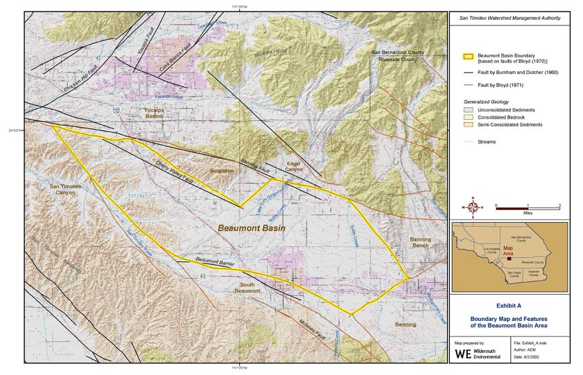
Figure A.1 in the Appendix shows the adjudicated boundaries of the Beaumont Basin following
2004. As is clear in the map, the adjudication only covered part of the region’s set of groundwater
basins. Appropriators included in the adjudication extracted groundwater from wells both inside and
outside the boundaries of the Beaumont Basin, both before and after the judgment. Their adjudicated
property rights only pertained to groundwater extracted from wells inside the Beaumont Basin. There
were overlying groundwater users with wells both inside and outside the boundaries of the Beaumont
Basin before and after the adjudication. Only overlying users inside the Beaumont Basin were given
adjudicated property rights. Thus, appropriator wells outside of Beaumont Basin and farmers located
outside of Beaumont Basin extract groundwater from basins that remain in open access during the
entire period of our data set, even after the institution of quantified property rights in Beaumont
Basin.
4.2 Data Sources
We rely on a number of sources. Summary statistics for data we have incorporated into our estimation
can be found in Tables A.1-A.3 in the Appendix.
First, for extraction data we use a mix of data from the San Timoteo Watershed Management
Authority, the San Gorgonio Pass Water Agency, and the Beaumont Basin Watermaster. Our ob-
servation for extraction is annual extraction by an owner either inside or outside the boundaries of
10the Beaumont Basin. Thus, for appropriators in the judgment we have two extraction observations
each year (i.e., extraction inside Beaumont Basin and extraction outside Beaumont Basin), while for
other extractors we have one observation per year (i.e., extraction either inside or outside Beaumont
Basin).
Second, we collect and construct a database of well characteristics and location for each owner in
each year from detailed handwritten hard-copy historical records on well location, well characteristics
such as the depth of the well, and the maximum extraction rate in gallons per minute from the
California State Water Resources Control Board’s Groundwater Recordation Program (California
State Water Resources Control Board, 2021). We merge the handwritten hard-copy historical records
wells location data from the Groundwater Recordation Program and a well completion report dataset
from the California Department of Water Resources with the well’s state well identification number to
determine the location of each the wells, and then merge the resulting well characteristics and location
data with reported data from the Beaumont Basin Watermaster and the San Timoteo Watershed
Management Authority. We map our well locations data to data from the USDA Web Soil Survey
and calculate an average saturated hydraulic conductivity value for each owner’s wells inside and
outside the Beaumont Basin; these data are fixed over time.
For data on depth to groundwater, we use observations from the US Geological Survey (USGS)
Historical observations dataset. We collapse our data into annual depth to groundwater near each
owner’s wells inside or outside the boundaries of the Beaumont Basin. In order to do this we average
over the nearest neighbor monitoring observations for each well owned by an owner either inside or
outside the basin. Thus each well owned by one of our groundwater extractors has a corresponding
monitoring well in the dataset. We interpolate for missing years in our depth to groundwater data
by using the inverse-distance weighted annual change in depth to groundwater at other nearby wells
with available data.
We obtain prices for relevant agricultural crops (apples, cherries, grapes, alfalfa, olives, and straw-
berries) from the USDA NASS Monthly Agricultural Prices survey. We use end-of-March surveys in
each year to map a price. We choose this month to correspond to the price data available at the time
of the planting decision for farmers. For our policy function and state transition estimation involving
electricity prices, we use data from the Southern California Edison on annual end-use price by sector.
For real GDP per capita, we use statewide annual data from the US BEA, with chained 1997 prices.
For data on unemployment rate and CPI, we use state-level data from the Federal Reserve Economic
Data supplied by the St. Louis Federal Reserve Bank. For county-level personal income, we use
data from the State of California Franchise Tax Board. We take prices for untreated water from the
Metropolitan Water District, a large State Water Project Contractor in Southern California. We take
equivalent use price and delivery data from the State Water Project’s annual Bulletin 132 report.
We make use of precipitation and daily maximum temperature data from the PRISM Climate
Group (PRISM Climate Group and Oregon State University, 2018). We use 4 km resolution data
from the PRISM’s historical dataset, and map it to the extraction wells in our dataset based on
11location. We then collapse our data into annual and growing season (April-October) averages across
wells inside or outside the Beaumont Basin for each owner.
In our demand estimation, we use data on per household monthly residential water demand, fixed
charge, variable price, and connection fee from the California/Nevada Water Rate Survey conducted
by the American Water Works Association. This survey is conducted once every two years and
covers a large sample of municipal water districts in California. We use data on household size and
population by city and county from the California Department of Finance; data on median adjusted
gross income by county from the California Franchise Tax Board; and data on the industrial average
electricity price for California from the US EIA.
5 Structural Econometric Model
To estimate the parameters for the open access dynamic game, we use the two-step forward simulation-
based approach developed by Bajari et al. (2007). In the first step of our estimation strategy, we
estimate a model of residential water demand, policy functions σi (x) for each player type, and state
transition densities for depth to groundwater. In the second step, we forward simulate estimates of
the value function at a set of states under policies and transition functions estimated in the first stage
and find parameters that minimize any profitable deviations from the optimal strategy as given by
the policy functions estimated in the first step. The estimated parameters are then consistent with
Markov perfect equilibrium behavior in a game in which player expectations are consistent with the
observed first-stage state transitions and policy functions (Bajari et al., 2007).
Finding a single equilibrium is computationally costly even for problems with a simple structure.
In more complex problems – as in the case of our dynamic game between groundwater users, where
many agents are involved – the computational burden is even more important, particularly if there
may be multiple equilibria. We apply the method proposed by Bajari et al. (2007) for recovering the
dynamic parameters of the payoff function without having to compute any single equilibrium. The
crucial mathematical assumption to be able to estimate the parameters in the payoff function is that,
even when multiple equilibria are possible, the same equilibrium is always played.
5.1 Residential Water Demand
As part of the first step of our estimation strategy, we empirically estimate the residential household
water demand function in equation (2), which is then used in the second stage of our estimator to
estimate consumer surplus and water sales revenue for water districts. Our observational unit here is
a water district in a given year. Our regression model is given by:
lnqi = α0 + α1 ln[Pi ] + α2 ln[fi ] + Xi0 α3 + i , (9)
12where qi is the quantity of household monthly water consumption in water district i; Pi is the resi-
dential water price in water district i; fi is the average household size in district i; and Xi is a vector
of controls, which include median per capita income, state-wide unemployment, precipitation, and
rate structure design.
Since residential water price is endogenously determined by both supply and demand for water,
we employ an instrumental variables approach, as is common in the literature on residential water
demand (Worthington and Hoffman, 2008). Here we instrument for the price of water with supply
shifters. Specifically, our instruments for price are the annual equivalent unit price charged by the
State Water Project (SWP) for water delivery to the water district’s nearest State Water Project
contractor, and the product of the average depth to groundwater in the district and the price of
electricity. These supply shifters are correlated with price because water district costs are generally
included in the pricing formula for the district. Since water districts draw on groundwater, surface
water, and water imports to meet their supply needs, these instruments clearly affect the cost of the
water district’s supply.
We believe that these instruments also satisfy the exclusion restriction. The State Water Project
(SWP) price for water delivery to the district’s nearest State Water Project contractor is determined
by the State Water Project, and reflects the costs of transporting water, obtaining supplies, and
maintenance (California Department of Water Resources, 2016b). Since the State Water Project does
not sell directly to water districts, but rather to large contractors who then sell water to the water
districts, no single district can fully determine the demands of a contractor, and the pricing rule used
by the SWP is not driven by the demands of any single contractor. Furthermore, differences across
contractors in price are driven mainly by differences in location, and the maintenance and capital costs
of the pipelines that transport water to each district. Thus, the State Water Project (SWP) price for
water delivery to the district’s nearest State Water Project contractor is a supply shifter that does not
affect residential water demand except through its effect on the residential water price. The average
depth to groundwater in the district interacted with the price of electricity is similarly a supply
shifter that does not affect residential water demand except through its effect on the residential water
price. We conduct several tests of both correlation and the exclusion restriction, and find evidence
that is consistent with our instruments being both relevant and valid. The Sanderson-Windmeijer
first-stage F-statistic (Sanderson and Windmeijer, 2016), which is a modification and improvement
of the Angrist-Pischke first-stage F-statistic (Angrist and Pischke, 2009), is equal to 199, which is
greater than the threshold of 10 used in current practice (Staiger and Stock, 1997; Stock and Yogo,
2005; Andrews et al., 2019), and also greater than the threshold of 104.7 for a true 5 percent test
(Lee et al., 2020).
For our water demand estimation, we use pooled data from the bi-annual California/Nevada Water
Rate Survey conducted by the American Water Works Association. We do not treat our data as a
panel due to the infrequency of repeated observations in our data. We use data on household size by
city and county from the California Department of Finance; data on median adjusted gross income
13by county from the California Franchise Tax Board; and data on the industrial average electricity
price for California from the US EIA. Our dataset covers the years 2007-2015. Summary statistics
are presented in Table A.3 in the Appendix.
Our empirical results for the residential water demand function can be found in Table 1. We find
elasticities of price and household size that fit with our prior belief that demand should be inelastic
with regard to each, and fit within the bounds of prior results in the literature (Worthington and
Hoffman, 2008). Since the coefficients on the variables in the vector Xi of controls are not significant
at a 5% level, we do not include these variables as determinants of water demand in our structural
model, but instead account for them by solving for the constant  that equates mean predicted
household consumption (using only price and household size as predictors) with actual consumption.
5.2 Policy Functions
For each type of player in our game, we estimate policy functions that correlate actions to states, using
data from the open access period of our dataset. These extraction policy functions are parametric
functions of state variables that are chosen based on their ability to accurately predict groundwater
extraction in sample. While we can not argue for the ability of these functions to predict extraction
outside of our sample set of states, we can evaluate our estimators based on the fit of our simulated
data with the actual data. Our policy function regression results can be found in Table 2.
We estimate policy functions for total extraction of groundwater by appropriators, farmers, and
recreational users. We estimate a separate policy function for the share of groundwater extraction at
wells inside the Beaumont Basin for water districts. In these models we control for depth to ground-
water, lagged extraction, physical features of the area surrounding the player’s wells, characteristics
of the wells and pumping technology, planned operational activities, prices, and weather conditions.
Our results, found in Table 2, show the significant coefficients in each model, which we then use in
our policy functions to simulate extraction choices. Since we only use a subset of variables included in
the estimated model, we choose a constant term that equates mean predicted extraction in each case
with mean actual extraction in the data. We account for unobserved factors that affect extraction
decisions using the root-mean squared prediction error from this adjusted predicted value and taking
a random normal draw.
5.3 State Transition Functions
We estimate transition densities for depth to groundwater for each type of player. We separately
estimate transition densities for depth inside and outside of Beaumont for water districts with wells
both inside and outside of the basin.
For the transition densities for depth to groundwater for each type of player, we estimate models
that include lagged depth to groundwater, extraction by the player, extraction by other players,
physical features of the area surrounding the player’s wells, prices, and weather conditions, and we
14let the data tell us what the transition density is. We only use variables that prove significant in our
state transition regressions in the second stage simulation. We adjust our constant to equate predicted
values with values in the data. We account for unobserved factors that affect state transitions using
the root-mean squared prediction error from this adjusted predicted value and taking a random
normal draw. Our transition densities for depth to groundwater are presented in Table 3.
For crop prices, well characteristics, and weather, we assume rational expectations by players in
the base case model. We relax this assumption in our robustness checks. We also assume that none of
our players can influence crop prices, well characteristics, or weather through their behavior. This is
a reasonable assumption given the relatively small size of operations in the Beaumont Basin relative
to other nearby population centers and agricultural operations.
5.4 Estimating the Structural Parameters
For the second step of our estimation strategy, following Bajari et al. (2007), we forward simulate the
value functions for each player in the open access period, and we estimate our structural parameters
θ by minimizing the sum of profitable deviations from the optimal strategy as estimated by our
policy functions. The structural parameters θ we estimate include revenue and cost parameters for
farmers, recreational users, and appropriators; and parameters governing the relative weights that
appropriators place on consumer surplus versus the profits from water sales. We set the discount
factor β to 0.9. To generate deviations from the optimal strategy, we perturb our policy functions
using random draws to increase and decrease the level of the policy function; these perturbations
are normally distributed with a standard deviation equal to the standard deviation of the relevant
player-type extraction decision in the data. To ensure that we find a global minimum, we iterate over
multiple initial guesses, searching over the set of combinations of parameter values, in order to find
the parameters that minimize the sum of profitable deviations.
Identification of the parameters in the marginal revenue and costs of extraction for each player
type (farmers, recreational users, appropriators) come from variation in extraction and state variables
across players and across years for each player type. Identification of the weights in the per-period
payoff on consumer surplus come from variation in water sale profits and consumer surplus across
appropriators and across years. Water sale profits depend on the revenue and costs of extraction,
whose parameters are identified from variation in extraction, number of high heat days, and precipi-
tation across appropriators and across years. Consumer surplus is calculated by integrating the area
under the inverse residential water demand above price, using the parameters in the residential water
demand function estimated in the first stage. Variation in consumer surplus comes from variation
in extraction, the number of households, and the average household size across water districts and
across years.
155.5 Calculating Welfare
We use our estimated structural parameters to calculate the welfare generated from groundwater
extraction under open access. Welfare is the present discounted value of the entire stream of per-
period payoffs over the period 1991-1996. Average annual welfare is welfare divided by the number
of years.
For each player and player type, we calculate the actual welfare generated based on the observed
player actions and state variables, the model predicted welfare generated from 100 simulation runs of
the open access period, and the difference between model predicted and actual welfare. Both actual
and model predicted welfare are calculated using the parameter estimates from the structural model.
Actual welfare is calculated using actual values of actions and states in the data. Model predicted
welfare is calculated using model predicted actions and states generated from 100 simulation runs of
the open access period.
In addition to welfare, we also calculate the actual consumer surplus faced by each appropria-
tor over the period 1991-1996 based on the observed player actions and state variables, the model
predicted consumer surplus generated from 100 simulation runs of the open access period, and the
difference between model predicted and actual consumer surplus. Consumer surplus is the consumer
surplus faced by each appropriator over the period 1991-1996. Average annual consumer surplus is
consumer surplus divided by the number of years. Both actual and model predicted consumer surplus
are calculated using the water demand parameter estimates. Actual consumer surplus is calculated
using actual values of actions and states in the data. Model predicted consumer surplus is calculated
using model predicted actions and states. Since consumer surplus is calculated from our first-stage
demand function and from values of the state and action variables, it therefore does not depend on
any structural parameters.
To further examine the welfare of players during open access, we also calculate and decompose
the profits for each player. Profits are calculated as revenues minus costs. Average annual profits,
revenues, and costs are the present discounted value of the entire stream over the period 1991-1996 of
profits, revenues, and costs, respectively, divided by the number of years. For farmers and recreational
users, average annual welfare is equal to average annual profits. For appropriators, profits are the
profits from water sales given by the water sale revenues minus extraction costs, while the per-
payoffs are a weighted quadratic function of consumer surplus and the profits from water sales. Both
actual and model predicted profit components are calculated using the parameter estimates from the
structural model. Actual profit components are calculated using actual values of actions and states
in the data. Model predicted profit components are calculated using model predicted actions and
states.
In addition to player welfare and consumer surplus, we also calculate social welfare. Social welfare
is equal to the sum of producer surplus and consumer surplus. For each player, producer surplus is
their profits from groundwater extraction: namely, the revenue from groundwater extraction minus
the costs of groundwater extraction. For farmers, golf courses and housing developments, producer
16surplus is equal to welfare. For appropriators, producer surplus is the profits from water sales, and ap-
propriator revenue is a weighted quadratic sum of producer surplus and consumer surplus. Consumer
surplus is the consumer surplus faced by each appropriator, and is not weighted by parameters in the
payoff function of the appropriator. We allow appropriators to apply unequal weights to producer
surplus and consumer surplus in their per-period payoff function. When calculating social welfare,
however, consumer surplus is weighted equally to producer surplus, or the sum of profits produced
from groundwater extraction by players in the game. Thus, social welfare may differ from the total
welfare over all players if appropriators do not put equal weights on producer surplus (or the profits
from water sales) and consumer surplus in their objective function.
6 Results
6.1 Structural Parameters
We now examine our structural parameter estimates from the open access dynamic game. The
parameter estimates for the coefficients on terms in the payoff functions for each player, as well as
the total average effect of key variables evaluated at the mean values of the variables in the data, are
reported in Tables 4-5.
For farmers, whose marginal revenue parameters are found in Table 4, we find that rainfall during
the dry season (which coincides with the growing season) increases the marginal value of extraction.
The coefficient in farmer marginal revenue on the interaction between crop price, number of high
heat days during the growing season, and precipitation during the growing season is significant and
negative, however, which means that additional growing season rainfall during a relatively warmer
year tends to lower the value of irrigation water. Thus, as expected, groundwater is more valuable to
farmers when rainfall does not meet the needs of their crops. Crop price in general lowers the marginal
revenue to farmers from irrigation, which is likely due to either expansion of farming activities to
more marginal land, or less productive increases in applied water during years in which crop prices
are relatively high: the total average effect is negative, and statistically significant. We find that the
total number of wells owned by the farmer has a significant positive effect on marginal revenue (likely
due to the ability to more agilely manage irrigation across space), and that this effect is amplified for
farmers inside the Beaumont Basin. We also find that farmers in the Beaumont Basin generally earn
higher returns on their groundwater extraction than their counterparts outside of Beaumont.
For golf courses and housing developments, whose marginal revenue parameters are found in Table
4, we find that rainfall during the dry season (which coincides with the growing season) increases the
marginal value of extraction. Here we see that the number of high heat days has a negative effect
on revenues, but a positive interaction with rainfall, suggesting that while hot days during a drought
may damage the profitability of applied groundwater, they improve it during relatively wetter years.
Results show that increased population and real income lead to more profitable extraction, likely due
to the effect these factors have on increasing overall demand for these overlying users’ services. We
17You can also read