Estimating the redshift of galaxies from their photometric colors using machine learning methods

Tecnología en marcha, Edición especial 2020
38          6th Latin America High Performance Computing Conference (CARLA)

     Estimating the redshift of galaxies
     from their photometric colors
     using machine learning methods
     Estimación del corrimiento al rojo para galaxias
     a partir de sus colores fotométricos usando
     métodos de aprendizaje automático
     Felipe Meza-Obando1

     Meza-Obando, F. Estimating the redshift of galaxies from
     their photometric colors using machine learning methods.
     Tecnología en Marcha. Edición especial 2020. 6th Latin
     America High Performance Computing Conference (CARLA).
     Pág 38-43.

          https://doi.org/10.18845/tm.v33i5.5073

     1   Doctorate in Engineering Candidate, Artificial Intelligence for Natural Science Lab (LIA-
         NA) and PAttern Recognition and Machine Learning (PARMA)- Instituto Tecnológico de
         Costa Rica (Thanks to Vicerrectoría de Investigación y Extensión (VIE) at Instituto Tecnó-
         logico de Costa Rica for supporting this research at LIANA.). E-mail: fmeza@tec.ac.cr.
            https://orcid.org/0000-0003-4239-3116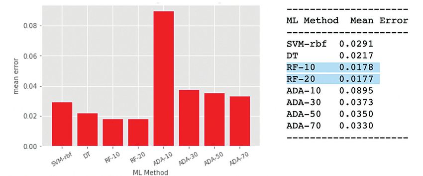

Tecnología en marcha, Edición especial 2020
                           6th Latin America High Performance Computing Conference (CARLA)            39

Keywords
Universe; expansion; redshift; galaxies; svm; decision trees; ada boost; random forest.

Abstract
The determination of the redshift, a factor also known as z, is obtained from variations in the
wavelength’s spectrum of galaxies or distant objects, such variation is basically the difference
between the wavelength measure on Earth of the element present in the galaxy and the direct
measure of the same element on the object by the use of spectroscopy. From the value z, it’s
possible to obtain the values of the object’s distance and the speed at which it moves away from
us. Obtaining spectroscopic data directly from astronomical objects, is not always an easy task
to run and the use of color index become a more accessible alternative for many researchers.
In this work we present the preliminary results of several machine learning methods, using
regression based algorithms. The goal will be to obtain the value of z, from the photometric
colors.

Palabras clave
Universo; expansión; desplazamiento al rojo; galaxias svm; árboles de decisión; bosque al azar.

Resumen
La determinación del corrimiento al rojo, factor conocido como z, se obtiene a partir de las
variaciones en la longitud de onda del espectro de la galaxia u objeto lejano, dicha variación se
da entre la medición en la Tierra del elemento presente en la galaxia y la medición directamente
en el objeto mediante espectroscopia. A partir del valor z, es posible obtener los valores de
la distancia del objeto y la velocidad a la que se aleja de nosotros. La obtención de datos
espectroscópicos en el objeto, no siempre resultan fáciles de obtener y los índices de color se
convierten en una alternativa más accesible para muchos investigadores, en este trabajo se
muestran los resultados preliminares de diversos métodos de aprendizaje automático, donde
como un problema de regresión y a partir de los índices fotométricos podemos estimar el valor
de z.

Introduction
Since the beginning of our universe 14 billions of years ago, the space around it has been
expanding, for this reason, the galaxies and other objects seem to be moving away from us at
specific rates. Due to the uniformity of such expansion, a direct relationship is present between
the speed of expansion of those galaxies and the distance from us. The resulting movement
of the expansion, as shown if figure 1, causes a shift in the frequency of photons that can be
visualized in the spectrum of the distant galaxies, since the universe is expanding away from us,
the shift is towards lower frequencies i.e red side of the spectrum, the effect is called redshift.
Spectral analysis consists in the measurement of the emission of photons at certain wavelengths
that can be represented as spectral lines in specific positions in the resulting spectrum, from
those lines one can determine the elements present in the object [2]. When astronomers
measure spectral lines in distant objects such as galaxies, lines appear to be shifted toward the
red side of the spectrum due to the difference between the wavelength measured on earth and
the one observed, the redshift is then defined by a value called z: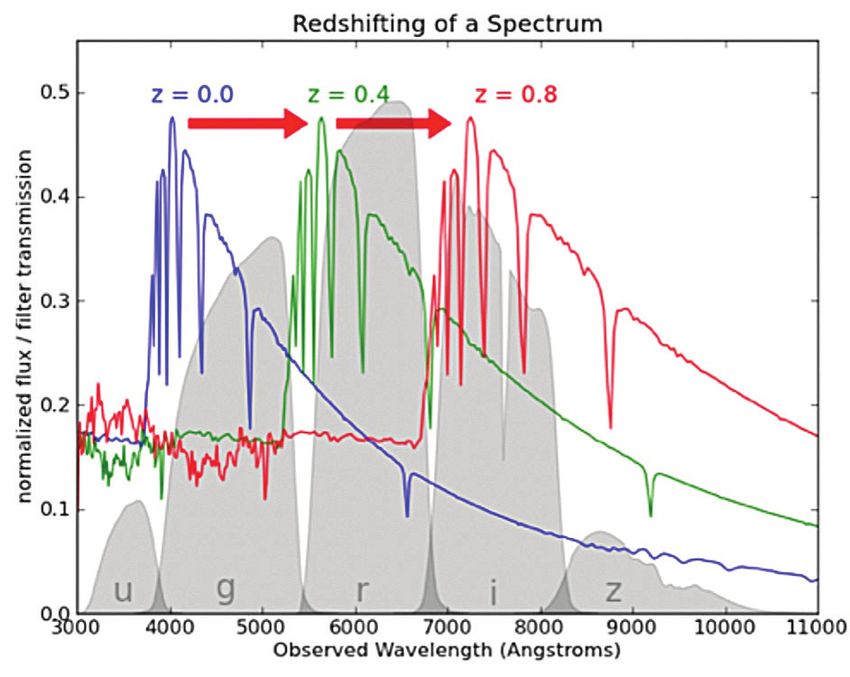

Tecnología en marcha, Edición especial 2020
40        6th Latin America High Performance Computing Conference (CARLA)

     From the redshift value z, it’s possible to obtain the velocity v at which the galaxy is moving away
     from us using the relation v = c × z, where c is the speed of light. Finally, with the value of v it’s
     also possible to estimate the distance of the galaxy using the Hubble Constant (HO=72 Km/s/
     Mpc) and the following relation d=v/HO

                   Figure 1. Comparison of different redshifts (Source: https://www.universetoday.com/)

     The conventional way to do this analysis is by the observation of the samples one by one of the
     resulting lines in the spectrums and calculate the observed shift, however with large amounts
     of data this process can be very time consuming and subjected to errors. On the other hand,
     not all the galaxies have all the spectral values related to the shift, for those reasons the use of
     machine learning results in a powerful and convenient option to estimate the values of z, from
     photometric colors.

     Machine Learning (ML) Algorithms
     We’ve chosen four basic supervised methods to estimate the value of z from the photometrics
     filters [3], which results in a very convenient way to estimate z since the observational data i.e
     color index is generally more available and easier to be obtained than the spectral data for such
     galaxies. The methods selected are briefly described [1], [5]:
        -		 Support Vector Machines (SVM): In this case is called Support Vector Regression (SVR),
            essentially a support vector (SV) is generated to follow the data trend and create the
            regression model.
        -		 Decision Trees (DT): This method maps a set of inputs features to their corresponding output
            targets, thanks to a series of individual decisions where each decision is represented by a
            node of the tree. Each decision node involves specific values, such values are determined
            from the training data in the learning algorithm based on the principle of “the most effective
            way to fit the data”.
        -		 Random Forest (RF): The goal is to have several random DT, each tree is created from
            random sets of samples from the data and each node is also created by selecting randomly
            the features to generate the best data fit.
        -		 AdaBoost (AB): Adaptive Boosting is based on the idea of having several weak classifiers
            or regressors to form together a much stronger and effective classifier or as in this case, a
            regressor.

Tecnología en marcha, Edición especial 2020
                              6th Latin America High Performance Computing Conference (CARLA)               41

Methodology and data
We use the spectrums from Sloan Digital Sky Survey catalogue (SDSS) [4], it’s of particular
interest the magnitude of the flux received in five bands (u, g, r, i and z). In astrophysics the
color index is the result of the difference between the magnitude of two filters i.e u-g, g-r, r-i and
i-z, those values will be our features. The u filter is near the blue side of the spectrum and the z
filter near the red side of the spectrum, if the spectrum is shifted to the red side then the value of
z will be larger, meaning that the galaxy is moving away from us. In figure 2 the blue spectrum
corresponds to the measurement at z=0 in other words our reference, however as the galaxy
is moving away the z value will be increased towards the red side, resulting in a speed v and
a distance d of the galaxy from our perspective. Our database was made up of samples with
values of flux in the u, g, r, i and z bands and is composed of 50000 galaxies; table 1 shows the
first and last three values of our dataset.

                      Figure 2. Redshifting of a spectrum (Source: https://scikit-learn.org/)

With the goal of making use of conventional ML algorithms to solve this regression problem, we
based our analysis in the measurement of the mean error as our metric:

                  Table 1. Samples from the database (Source: original dataset from SDSS)

    ID            u                 g                 r                  i                z      redshift
     0        19.84132          19.52656          19.46946          19.17955          19.10763   0.539301
     1        19.86318          18.66298          17.84272          17.38978          17.14313   0.164570
     2        19.97362          18.31421          17.47922          17.07440          16.76174   0.041900
   49997      19.82667          18.10038          17.16133          16.57960          16.19755   0.078459
   49998      19.98672          19.75385          19.57130          19.27739          19.25895   1.567295
   49999      18.00024          17.80957          17.77302          17.72663          17.72640   0.474945

Tecnología en marcha, Edición especial 2020
42        6th Latin America High Performance Computing Conference (CARLA)

     Results

     In the experiments, we used scikit-learn framework to run a comparison between the four
     proposed methods. In the case of SVM, the kernel used was rbf (SVM-rbf), with decision trees
     (DT) we used the depth as our hyperparameter, even with the use of several depth values the
     results remain almost the same. With Random Forrest we used two references values for the n_
     estimators hyperparameter, 20 and 100 (RF-20 and RF-100), beyond the value of 200 the results
     seems to have no major variations, finally with Ada Boost we did the same setting as with RF to
     create two models (ADA-20 and ADA-100). Considering that the value of z is mostly in a range
     between 0 and 1 in our database, the mean error obtained for the all the methods varied from
     0.001 to 0.003, in the order of 10-3 a variation between 10 and 30, that represent a good result
     considering this as our first approach, however RF algorithm was the one that delivered the best
     result of 0.001, for this reason is considered the best result. In the case of ada boost method,
     one particular experiment using the hyperparameter n_estimators with a value of 10, resulted
     in the poorest mean error in the margin of 0.008, not bad at all but the lowest obtained from the
     experiments. As expected SVM reached the highest computational cost, due to the nature of the
     algorithm. The results obtained in regards to the mean error are shown in figure 3. In terms of the
     time consumed per algorithm, all the measurements were taken using the same computer: Apple
     MacBook Pro 2015 with processor 2.5 GHz Intel Core i7 and 16 GB 1600 MHz DDR3 memory, as
     expected SVM-rbf was the highest in terms of computational cost and RF was not just the best in
     terms of the mean error but also one of the most effective (RF-20) in terms of computational cost.

                  Figure 3. Mean error of the redshift in the galaxies, using the ML proposed methods.

Tecnología en marcha, Edición especial 2020
                                6th Latin America High Performance Computing Conference (CARLA)           43

                                 Figure 4. Time consumed per each ML method.

Conclusions and future work
The regression methods selected for the series of experiments resulted in a good approach to
estimate the redshift value z, the use of mean error represented also a good metric due to the
nature of the regression model. Even with the good results obtained with the proposed methods,
actual analysis is concentrated in the minimization of the mean error through the use of artificial
neural networks, another potential improvement to the model consist in the inclusion of more
data to the current dataset as it become available. Other tasks are concentrated in the analysis
of variations in the splitting of the dataset in order to validate and measure any overfitting effects
on the results.

References
[1]   S. Marsland, “Machine Learning: An Algorithmic Perspective”, 2nd Edition, C&H/CRC, 2014.
[2]   J. Rich, “Fundamentals of Cosmology”, Springer-Verlag Berlin Heidelberg, 2010.
[3]   C. Davis, et al., “Accurate redshift estimation from photometric colors”. Physics Stanford. 2013.
[4]   Sloan Digital Sky Survey, Data Access, Retrieved from https://www.sdss.org/ , January 2019.
[5]   E. Alpaydin, “Introduction to Machine Learning”, 2nd Edition, The MIT Press, 2016.