Determining spatio temporal characteristics of coseismic travelling ionospheric disturbances (CTID) in near real time - Nature
←
→
Page content transcription
If your browser does not render page correctly, please read the page content below
www.nature.com/scientificreports
OPEN Determining spatio‑temporal
characteristics of coseismic
travelling ionospheric disturbances
(CTID) in near real‑time
Boris Maletckii* & Elvira Astafyeva
Earthquakes are known to generate ionospheric disturbances that are commonly referred to as
co-seismic travelling ionospheric disturbances (CTID). In this work, for the first time, we present
a novel method that enables to automatically detect CTID in ionospheric GNSS-data, and to
determine their spatio-temporal characteristics (velocity and azimuth of propagation) in near-real
time (NRT), i.e., less than 15 min after an earthquake. The obtained instantaneous velocities allow
us to understand the evolution of CTID and to estimate the location of the CTID source in NRT.
Furthermore, also for the first time, we developed a concept of real-time travel-time diagrams that
aid to verify the correlation with the source and to estimate additionally the propagation speed
of the observed CTID. We apply our methods to the Mw7.4 Sanriku earthquake of 09/03/2011 and
the Mw9.0 Tohoku earthquake of 11/03/2011, and we make a NRT analysis of the dynamics of CTID
driven by these seismic events. We show that the best results are achieved with high-rate 1 Hz data.
While the first tests are made on CTID, our method is also applicable for detection and determining
of spatio-temporal characteristics of other travelling ionospheric disturbances that often occur in the
ionosphere driven by many geophysical phenomena.
It is known that natural hazard events, such as earthquakes, tsunamis and/or volcanic eruptions generate acoustic
and gravity waves that propagate upward in the atmosphere and ionosphere (e.g.,1–7). Earthquake-driven iono-
spheric disturbances are called co-seismic travelling ionospheric disturbances (CTID). The first CTID are gener-
ated directly by the ground or the seafloor via acoustic waves, they reach the ionospheric altitudes (~ 200–350 km)
in only 7–9 min. They are followed by acoustic waves generated by the surface Rayleigh waves, and tsunami
gravity waves. Nowadays, with the development of permanent networks of dual-frequency Global Navigation
Satellite Systems (GNSS) receivers, the detection of CTID and other Natural-Hazard-driven (NH-driven) iono-
spheric perturbations has nowadays become quite regular (e.g.,5,8–12).
Recently, it has been suggested that NH-driven ionospheric disturbances can be used for more advanced
purposes: to localize NH and to estimate the characteristics of the source (e.g.,13–19). Kamogawa et al.20 sug-
gested a method based on observations of a “tsunami-ionospheric hole”, ionospheric depletion that often occurs
after major earthquakes over the epicentral area. Based on the analysis of seven tsunamigenic earthquakes in
Japan and Chile, Kamogawa et al.20 found a quantitative relationship between the initial tsunami height and
the TEC depression rate. Manta et al.21 developed a new ionospheric tsunami power index based on measure-
ments of CTID. They showed that the ionospheric index scales with the volume of water displaced due to an
earthquake. However, neither of these methods is real-time compatible. As near-real-time (NRT) mode, we refer
to as 10–15 min after an earthquake. Going further towards NRT, Savastano et al.22 made the first preliminary
feasibility demonstration for ionospheric monitoring by GNSS, by developing a software VARION that can
derive TEC in NRT. Their technique has been implemented at several GNSS-receivers around the Pacific Ocean
(https://iono2la.gdgps.net), and is aiming—in the future—to detect traveling ionospheric disturbances (TID)
associated with tsunamis. Shrivastava et al.23 demonstrated the possibility of tsunami detection by GPS-derived
TEC, however, no discussion on the real-time use was provided.
Ravanelli et al.24 claimed to provide the first real-time ionosphere-based tsunami risk assessment by data
GNSS receivers in Chile. However, they analyse 2 h of data and used 8th order polynom, i.e., their approach
requires stacking of about 2 h of data. Therefore, this approach is not NRT-compatible by our definition.
CNRS UMR 7154, Institut de Physique du Globe de Paris (IPGP), Université de Paris, 35‑39 Rue Hélène Brion,
75013 Paris, France. *email: maletckii@ipgp.fr
Scientific Reports | (2021) 11:20783 | https://doi.org/10.1038/s41598-021-99906-5 1
Vol.:(0123456789)
www.nature.com/scientificreports/
Figure 1. Real-time collection of GNSS phase data and orbit parameters. Networked Transport of R TCM26 via
27
Internet Protocol (NTRIP) could be used to provide the real-time data stream from GNSS stations. The main
goal of the protocol is Real Time Kinematics (RTK), but it is also suitable for our purposes since it transfers
dual-frequency phase and pseudo-range data in real time. RTKLib28 software could be used to convert binary
information from NTRIP data stream. The International GNSS Service (IGS) ultra-rapid o rbit29 is used to obtain
the information about the elevation angle and the azimuth. BINEX Binary INdependent EXchange format for
files that is used in real-time.
Therefore, recent seismo-ionospheric results show a big potential for the future use of ionospheric meas-
urements for natural hazard risk assessment. However, before such methods could be applied in real-time,
several major developments are yet to be implemented. Going toward real-time applications, the first step is
to automatically detect CTID in near-real-time and to analyze their features in order to prove their relation to
earthquakes. In this work, we introduce, for the first time, near-real-time compatible methods for determining
the spatio-temporal characteristics of CTID.
Methods
Estimation of total electron content (TEC) from GNSS. GNSS allows to estimate the ionospheric
total electron content (TEC), which is an integral parameter equal to the number of electrons along a line-of-
sight (LOS) between a satellite and a receiver. The LOS TEC is often called slant TEC (sTEC). The TEC is usually
measured in TEC units (TECU), with 1 TECU equal to 1016 electrons/m2. To calculate the TEC, one needs phase
and code measurements performed by dual-frequency receivers (i.e.,25). However, the code measurements are
only needed to remove the inter-frequency bias. While, the co-seismic signatures and other disturbances can be
retrieved from phase TEC estimated solely from phase measurements:
1 f 2f 2
sTEC_ph = · 2 1 2 2 (L1 1 − L2 2 ) (1)
A f1 − f2
where A = 40.308 m3/s2, L1 and L2 are phase measurements, λ1 and λ2 are wavelengths at the two Global Position-
ing System (GPS) frequencies (1575,42 and 1227,60 MHz). Therefore, in near-real-time approach, we will only
use these phase measurements that can be easily transferred in very short time (Fig. 1). The first data point is
removed from the whole data series as the unknown bias.
In order to determine the position of ionospheric disturbances, we estimate the coordinates of so-called sub-
ionospheric points (SIP) that represent the intersection points between the LOS and the ionospheric thin shell.
The satellite orbit information can be rapidly transferred in NRT from the IGS in navigation RINEX files (Fig. 1),
or it can be forecasted very precisely based on the current known satellite coordinates. Otherwise, ultra-rapid
orbits can be used. The shell altitude Hion is not known but presumed from physical principles: we expect the
observed perturbation to be concentrated at the altitude of the ionization maximum (HmF2). In NRT, the value
of HmF2 can be obtained either from nearest ionosonde stations, or from empirical ionospheric models, such
as NeQuick30 or International Reference Ionosphere (IRI)31. Here we take Hion = 250 km, which is close to the
HmF2 on the days of the earthquakes15,32.
It should be noted that in the vast majority of previous studies of ionospheric response to earthquakes
the researchers used band-pass filters, such as running mean, polynomial fitting, high order Butterworth, etc.
(e.g.,33–35). However, in a real-time scenario one cannot use such filters because of the impossibility to stack long
series of data (up to 30–60 min) and due to the lack of time. In addition, the band-pass filtering would induce
artefacts and will affect the properties of the detected signals (arrival time, amplitude, spectral components).
Therefore, here we suggest to analyze the rate of TEC change (dTEC/dt) instead of the sTEC. Such a derivative
procedure works as a high-pass filter and removes the bias and trend caused by the satellite orbit motion. In
addition, our dTEC/dt approach will not modify the amplitude of CTID.
Scientific Reports | (2021) 11:20783 | https://doi.org/10.1038/s41598-021-99906-5 2
Vol:.(1234567890)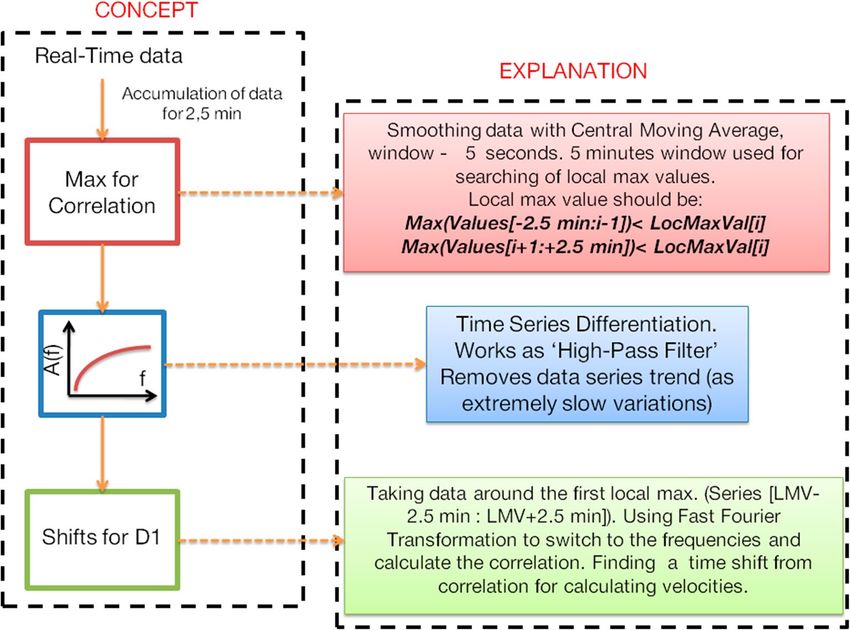
www.nature.com/scientificreports/
Figure 2. The concept of the near-real-time detection of CTID and TID, and explanation of the main steps of
the procedure.
Below we use 1 Hz GNSS data for our real-time scenario.
Real‑time detection of co‑seismic travelling ionospheric disturbances from TEC data
series. The concept of the developed method is presented in Fig. 2. CTID are detected by analysing the sTEC
data series by 5-s centered moving averaged over a 5-min window. The averaging prevents detection of random
peaks in data. The window duration is chosen to be NRT-compatible and, at the same time, it allows more thor-
ough analysis of CTID characteristics in multiple data series at later steps. Within the selected time window, we
search for a local maximum value (LMV) that must exceed every other value within the window.
At step #2, within the window, we switch from sTEC to dTEC/dt. With such an approach, we focus on sud-
den strong co-seismic TEC signatures that are analogous to the peak ground d isplacements36. Figure 3a shows
examples of CTID detected by GPS stations 0980, 3007 after the 2011 Tohoku-oki earthquake (1 Hz data). The
co-seismic signatures in sTEC data series (panels a, b) are quite significant, however, the presence of the trend
makes it difficult to calculate the correlation function and the time shift between the data series that are neces-
sary at later steps. In turn, in the dTEC/dt data series, the CTID signatures are visible, but the trend is removed
(Fig. 3c). The chosen 5-min window is enough to compute the correlation, since it catches the CTID signatures
and they prevail in the time span.
At step #3, we compute the cross-correlation function for two data series in order to obtain the time shifts in
the signal arrivals. The latter is found based on the maximum of the cross-correlation function. In addition, the
cross-correlation can correct possible errors in finding the LMV. Finally, from the obtained maximum values, it
can select 3 GNSS stations for the D1- technique, as explained below in P.3.
To calculate the cross-correlation function, we use Fast Fourier Transformation (FFT), which is a rapid pro-
cedure and suitable for NRT applications. Figure 3d shows an example of the cross-correlation function between
dTEC/dt data series at two GPS receivers.
The threshold for the correlated data series depends on the standard deviation of dTEC/dt series:
T = 1 − (1 − K ∗ σ1 ) ∗ (1 − K ∗ σ2 ) (2)
where σ1 , σ2—the standard deviation of dTEC/dt series at GNSS sites. The standard deviation is an indicator of
data noisiness. The noisier the data the more difficult it is to detect CTID because of a lower correlation coef-
ficient. Therefore, our approach will adaptively consider the data noise level. Another issue in determining the
threshold T is linked with different data cadences. The dTEC/dt values will increase with data cadence. Conse-
quently, to adapt the threshold estimation to different data sampling, we introduce a normalizing coefficient K.
For 1-Hz data, the K is chosen to be 10 T ECu−1 based on data analysis. Such an adaptive approach makes our
method adjustable to the scale of an ionospheric response and aids to automate the triangle selection process (at
a later step). It is known that smaller earthquakes generate CTID of smaller amplitudes51. When the response
Scientific Reports | (2021) 11:20783 | https://doi.org/10.1038/s41598-021-99906-5 3
Vol.:(0123456789)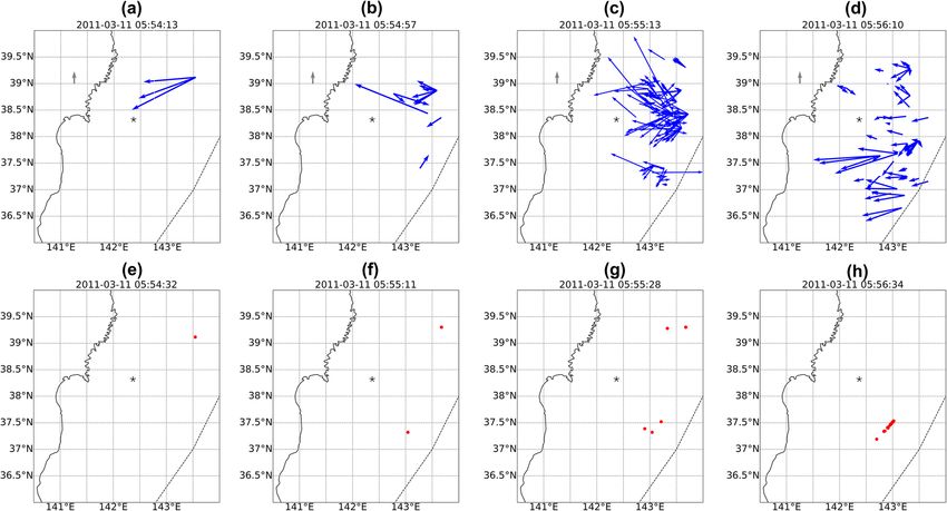
www.nature.com/scientificreports/

                                            Figure 3.  (a) Variations of slant TEC registered by GPS satellite 26 at stations 0980 and 3007 following the
                                            Tohoku earthquake of 11 March 2011. The earthquake time is indicated by vertical black line. Gray shaded
                                            rectangles denote 5-min time window, which is used for further cross-correlation analysis; (b) sTEC variations
                                            within 5-min time window; (c) dTEC/dt within 5-min time window. Black point shows the LMV determined
                                            from the sTEC data. The data are 1 Hz; (d) Cross-correlation function for the two dTEC/dt time series.

          Scientific Reports |   (2021) 11:20783 |              https://doi.org/10.1038/s41598-021-99906-5                                                   4

Vol:.(1234567890)
www.nature.com/scientificreports/
Figure 4. (a) Explanation of D1 technique. A, B, C—GNSS stations that are used to determine the CSID
parameters: horizontal velocity (vh) and azimuth (α). 0, I, II, III mark the moments of time when the
perturbation approaches the detection triangle (0) and when the perturbation is detected at points A, B, and C,
respectively. The wavefront is considered to be plain; (b) Ionospheric localization of CTIDs based on the known
location and values of two velocity vectors V
1 and V2 as determined by using the D1-method
is weaker, the threshold is smaller due to the smaller standard deviation of dTEC/dt series and vice versa. (Fig-
ure S1). Setting a constant threshold may affect the results and that there is a need for an adaptive algorithm for
this problem.
Real‑time estimation/determining of spatio‑temporal parameters: D1‑GNSS‑RT method. To
determine spatio-temporal parameters of CTID, such as the horizontal velocity and the azimuth of propagation,
we use a so-called “D1” method. This is an interferometric approach that was introduced by Afraimovich et al.37
to analyze and detect TID, of which CTID are a subclass. Originally, this method was based on use of GPS-
measurements only37,38. Our method works with all GNSS data, and it is real-time compatible, therefore, we refer
to it as “D1-GNSS-RT”.
The disturbances detected by a system of three spatially separated receivers, that act as an interferometric
system, are considered to be parts of the same wavefront (Fig. 4a). Then, by analysing the wave characteristics
(such as phase, frequency, signal amplitude) of the observed disturbances, we determine the time shift between
CTID arrivals at the detection “triangle”. Three assumptions are used in the subsequent calculations: (1) the wave
front is plane, i.e., the distance between the receivers is less than the horizontal dimensions of CTID; (2) the
wave front is homogenous; (3) the CTID propagate horizontally i.e. the GNSS-receivers detect the perturbations
at the same altitude (Hion).
At the “0” time moment, a disturbance with horizontal velocity vh and azimuth α is approaching the “A–B–C”
interferometric system. At the moment “I”, the CTID is detected by the receiver “A”, and it is further moving
to other receivers of the system. It is important to note that the consideration of the wave front as plane and
homogeneous means that both vh and α would not change when the CTID arrives at the other points of the given
system. Garrison et al.39 showed the correctness of such an assumption for small-scale (3–10 min) TIDs, based
on the dense network of receivers in the limited space. At moment “II”, the CTID has already passed receiver
“A”, and arrived at receiver “B”. At “III”, the CTID arrives at receiver “C”. Only after this step, one can compute
the characteristics of the perturbation. The velocity vh and the azimuth α are then estimated by using the fol-
lowing formulas40:
xA ∗ yC − xC ∗ yA
ux =
yC ∗ (tA − tB ) − yA ∗ (tC − tB ) (3)
xA ∗ yC − xC ∗ yA
uy =
xA ∗ (tC − tB ) − xC ∗ (tA − tB ) (4)
ux ∗ uy
vh =
ux2 + uy2 (5)
Scientific Reports | (2021) 11:20783 | https://doi.org/10.1038/s41598-021-99906-5 5
Vol.:(0123456789)
www.nature.com/scientificreports/
uy
tan α =
ux (6)
For better spatial representation, the location of the obtained horizontal velocity vector is placed at the point
with the first arrival of the disturbance (point A in Fig. 4a). While, in the temporal domain, the obtained velocity
is linked with the arrival time of the disturbance at point C.
As mentioned before, the D1-method is only applicable to a TID with a plain waveform. It is known however
that, in most cases, the wave front of CTID is circular (e.g.,5,41). Therefore, the farther are the stations from one
other, the worse is the plain wave condition fulfilled. Also, larger distance between the stations will lower the
maximum of the cross-correlation function. Consequently, the D1-GNSS-RT can only be used on a very small
segment of the circular wavefront. This limitation requires additional analysis of the positions of the A, B, C
receivers with respect to the wavefront. To do that, here we use the cross-correlation function that is the criterion
of the similarity of multiple data series. It should be noted that the waveform of the CTID largely depends on
the conditions of observations, such as magnetic field configuration in the epicentral area, geometry of GNSS-
sounding and the background ionization (e.g.,41–44). Therefore, only perturbations registered close to one another
will have similar waveforms.
Localization of the source of ionospheric disturbances. The velocity field obtained by the D1-GNSS-
RT method can further be used to locate the source of CTID. The source is defined as a point in the ionosphere
where the CTID is generated and starts to propagate horizontally outward from the source. We switch to Lati-
tude–Longitude coordinate system, where x-axis is directed from West to East and y-axis is directed from North
to South (Fig. 4b). We take the azimuths (αi) and the values (vi) of the velocities, as well as the coordinates (lon0i
and lat0i ) of the velocity “vectors” from the output of the D1-GNSS-RT. This gives us a linear system, where the
coordinates (lon0 and lat0) of the source of ionospheric disturbances are unknown. There are two additional
restrictions on the system solutions: (1) the horizontal distance between the vectors should be less than 50 km
and (2) the difference in the arrival times between points A–B and A–C should be less than 30%. These restric-
tions are thought to avoid the location of velocity vectors to be on the same segment of the CTID wavefront in
order to fulfill the condition of the plain wavefront.
For one velocity vector the distance to the source is defined by the following equation (Fig. 4b):
lon0 − lon0i = tan (αi ) ∗ (lat0 − lat0i ) (7)
where lon0 and lat0—the coordinates of the source, lon0i and lat0i—that of the given velocity vector, αi—the
azimuth of the velocity vector. Similarly, for two vectors we obtain:
lon0 = tan (α1 ) ∗ (lat0 − lat01 ) + lon01
lon0 = tan (α2 ) ∗ (lat0 − lat02 ) + lon02 (8)
Based on the system above, the coordinates of the intersection of the two vectors can be estimated as:
lat0 = (lon02 −lon01 )+(lat01 ∗tan (α1 )−lat02 ∗tan (α2 ))
tan (α1 )−tan (α2 ) (9)
lon0 = lon01 + tan (α1 ) ∗ (lat0 − lat01 ) or lon02 + tan (α2 ) ∗ (lat0 − lat02 )
Once the source location is known, along with the velocity vector location and its value, the onset time of
the source is estimated as follows:
t = ti + ti (10)
where ti is the time of the velocity vector and ti is defined by:
Dist(lon0 , lat0 , lon0i , lat0i )
�ti = (11)
vi
where Dist(lon0 , lat0 , lon0i , lat0i ) is the distance between the source location and the velocity vector location. If
the difference in determination of the source onset time from the two given velocities is less than the sampling
interval, we consider this pair of velocities as a possible solution for a specific moment of time and location of
the source.
Results
We apply our newly developed methods to the cases of two shallow (~ 32 km) earthquakes that occurred in
March 2011 off the east coast of Honshu, Japan. The first one is the great M9.1 Tohoku-oki earthquake. Accord-
ing to the US Geological Survey (The National Earthquake Information Center (NEIC); http://earthquake.usgs.
gov), the epicenter of this earthquake was located at 38.322° N and 142.369° E (Fig. 5a), and the onset time was
estimated at 05:46:26 UT. The rupture lasted about 180 s, and caused significant co-seismic cumulative slip with
the maximum of 56 m on the north-east from the epicentre (Fig. 5a)45. Several research groups pointed out
that the Tohoku earthquake slip consisted of 2 or 3 “segments” (e.g.,46,47), that present multiple sources for the
ionospheric disturbances (e.g.,19).
The second event is the M7.3 Sanriku-oki earthquake that occurred 55 h before the Tohoku earthquake (i.e.,
on 9 March) and is often referred to as the Tohoku foreshock. According to the USGS, the rupture started at
02:45:20 UT at the epicentre with coordinates: 38.435° N, 142.842° E (Fig. 5b). This smaller event lasted 30–40 s
and provoked a 2 m co-seismic slip on the north-west from the epicentre (Fig. 5b)49.
Scientific Reports | (2021) 11:20783 | https://doi.org/10.1038/s41598-021-99906-5 6
Vol:.(1234567890)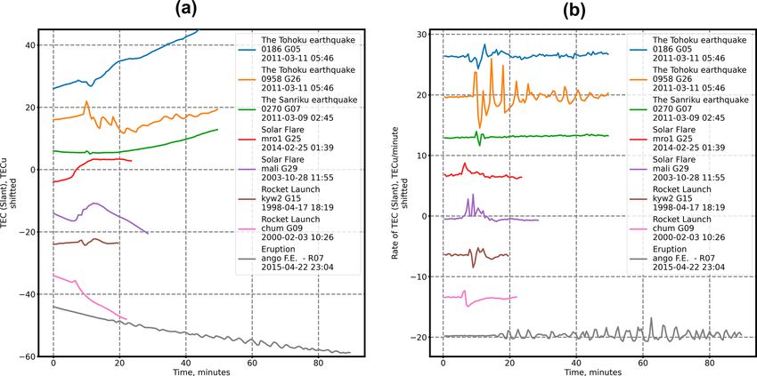
www.nature.com/scientificreports/
Figure 5. Maps for the Mw9.0 Tohoku earthquake of 11 March 2011 (a) and the M7.3 Sanriku earthquake of 9
March 2011 (b). Black star shows the epicenter, black dots show GPS receivers, and the colored squares depict
SGS41. The
the amplitude of the co-seismic slip that occurred due to the earthquakes as calculated by the NEIC U
corresponding color scale is shown on the bottom. The dotted curve shows the position of the Japan Trench. The
maps were plotted by using GMT6 software48.
To analyze the CTID activity, in both cases, we apply our method to 1 Hz GNSS ionospheric data from the
Japan GNSS Earth Observation Network (GEONET, https://www.gsi.go.jp).
The velocity field and ionospheric localisation of the 2011 M9.1 Tohoku‑oki earthquake. The
ionospheric response to the Tohoku earthquake was studied in detail by numerous research teams (e.g.,5,6,14,15,19,50).
As shown in Fig. 3, the near-field TEC response showed very complex waveforms, with several peaks in TEC
data. The amplitude of this response was also quite significant as compared to other earthquakes and was
detected by ten GPS satellites5,6,34,35. Here we work with data of GPS satellite 26 that showed the largest and the
clearest co-seismic signatures.
The CTID velocity field maps for the first CTID arrivals following the Tohoku earthquake are shown in
Fig. 6a–d, and the localization results are shown in Fig. 6e–h. It should be noted that, in principle, we can cal-
culate the CTID characteristics for multiple periods of time, as long as the perturbations are detected. For the
Tohoku event, instantaneous velocity maps for the first 2 min of CTID detection can be found in Animation S1
(available as supplementary material), and the localization results are shown in Animation S2 (supplementary
material). Figure 6a shows the first velocity vectors at 05:54:13UT, i.e. 487 s after the earthquake onset time, on
the north-east from the epicenter. The first vectors are directed south-westward, and the first points have the
velocities of about 4 km/s. Such velocity values might correspond to the propagation of the primary (P-) seismic
waves (i.e., the rupture propagation), or to the propagation of the Rayleigh surface waves. These first velocity
vectors give the first source location at the point with coordinates (38.18; 143.55) (Fig. 6e). At 05:54:57UT, one
can see further development of the CTID evolution within the source area, with smaller velocities. In addition,
we notice the occurrence of the second source on the south-east from the epicentre (Fig. 6b, f). Further, one can
clearly see the occurrence of the second segment of the source on the south-east from the epicenter (Fig. 6d, g).
At 05:56:10UT, we observe further evolution of CTID, and westward propagation of CTID with velocities from
600 m/s to ~ 3 km/s. This range of velocities was previously observed for the CTID generated by the Tohoku
earthquake (e.g.,5,6,14).
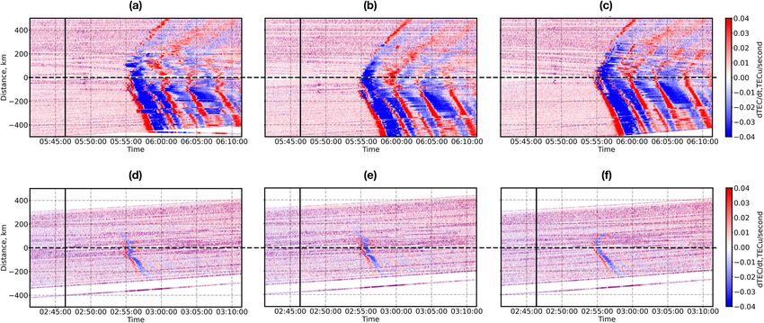
The CTID propagation speed can be verified by plotting so-called travel-time diagrams (TTD), that present
3-D diagrams with the distance from the source versus time after the source onset, and the amplitude of CTID
is shown in color. TTD also enable to confirm the correlation of the observed perturbations with the source.
In retrospective studies, a band-pass filter was applied in order to better extract the co-seismic signatures and
to clearly see the correlation with the source. In NRT mode, and with the impossibility to use such a filter, we
suggest using dTEC/dt parameter, and we call such diagrams near-real-time TTD (NRT-TTD). This is the first
NRT-compatible method proposed for obtaining the TTD. As a source, at the first approximation, we can take the
epicentre position that should be known from seismological data several minutes after the earthquake. However,
the epicentre is the point where the rupture starts, and its position does not always correspond (especially for
large earthquakes) to the position of the co-seismic crustal uplift that generates CTID as well as tsunamis. The
Scientific Reports | (2021) 11:20783 | https://doi.org/10.1038/s41598-021-99906-5 7
Vol.:(0123456789)
www.nature.com/scientificreports/

                                            Figure 6.  (a-d) CTID velocity field calculated from the first CTID detected by GPS satellite PRN 26 after the
                                            Tohoku earthquake. The dotted curve shows the position of the Japan Trench, black star depicts the epicenter.
                                            The gray arrow corresponds to 1.1 km/s; (e–h) localization of the seismic source as estimated from the first
                                            velocity vectors shown on panels (a–d).

                                            Figure 7.  Near-real-time travel time diagram (NRT-TTD) plotted by using dTEC/dt data for the Tohoku (a–c)
                                            earthquake (satellite G26) and Sanriku (d–f) earthquake (satellite G07). In panels (a, d) the distance is calculated
                                            with respect to the earthquakes’ epicenters as estimated by the USGS, in panels (b, e)—with respect to the
                                            maximum co-seismic uplifts; (c, f)—with respect to the ionospheric localization as shown in Fig. 5d, e and 6d, e.
                                            The color scale is shown on the right.

                                            problem lies, however, in the fact that in NRT, it is very difficult to know the position of the uplift or the slip.
                                            Therefore, we can take the position of the source estimated from our ionospheric methods.
                                                The NRT-TTD for the Tohoku event, G26 satellite, plotted for the source located at the epicentre, the center
                                            of the maximum slip (38.64; 143.35) and the “ionospheric source” (37.944; 143.153) are presented in Fig. 7a–c,
                                            respectively. It should be noted that the Tohoku earthquake produced significant displacement of the ground
                                            on a large area (the approximative fault size is about 300*80 km) and, strictly speaking, taking a single point as

          Scientific Reports |   (2021) 11:20783 |               https://doi.org/10.1038/s41598-021-99906-5                                                   8

Vol:.(1234567890)
www.nature.com/scientificreports/
Figure 8. (a–d) CTID velocity field calculated from the first CTID detected by GPS satellite PRN 07 following
the Sanriku earthquake. The dotted curve shows the position of the Japan Trench, black star depicts the
epicenter. The gray arrow corresponds to 1.1 km/s; (e–h) localization of the seismic source as estimated from the
first velocity vectors shown on panels (a–d).
the source is an approximation. However, we proceed with such an assumption to plot the NRT-TTD. The cor-
relation is seen when CTID propagates “linearly” from the source. Comparison of Fig. 7a–c reveals that the best
correlation is obtained for the slip maximum (Fig. 7b) and for the ionospherically-determined source (Fig. 7c).
While, the perturbation is not well-aligned when the diagram is plotted with respect to the epicentre (Fig. 7a).
The propagation speed of the observed CTID can be estimated from the slopes on the TTD. We find the speeds
to be ~ 2.3–2.6 km/s, which is in line with previous retrospective observations for the ionospheric response to
the Tohoku earthquake (e.g.,5,6,14,15).
The velocity field and ionospheric localisation of the 2011 M7.3 Sanriku‑oki earthquake. Iono-
spheric response to the Sanriku earthquake was studied previously by Thomas et al.53 and Astafyeva and S hults32.
The co-seismic TEC signatures were detected by satellites G07 and G10. Here we only focus on CTID registered
by GPS satellite G07. Contrary to the CTID generated by the Mw9.0 Tohoku earthquake, the ionospheric TEC
response to this smaller earthquake presented the commonly known N-wave signatures with smaller ampli-
tudes. However, even despite the smaller amplitude of CTID, our method detects these disturbances.
The instantaneous velocity field maps are presented in Fig. 8a–d. One can notice that the picture of the velocity
field for the CTID generated by the Sanriku event is much simpler that the one for the Tohoku event. The first
velocity vector is shown at 02:55:08UT, i.e. 588 s after the earthquake onset time. At that instant, the CTID starts
to propagate south-westward at the velocity of about 850 m/s (Fig. 8a). Within the next minute, we observe south-
westward propagation of ionospheric disturbances at ~ 850–1100 m/s (Fig. 8b, c). At 02:56:08UT, we observe
further southwestward propagation of CTID (Fig. 8d). From these first velocity fields, we estimate the location
of the source to be on the south-east from the epicentre (Fig. 8e–h). Overall, one can notice significant difference
in the velocity field and CTID evolution during this smaller earthquake. The CTID have lower velocities, and
the velocity field is much less complex as compared to the Tohoku earthquake.
The corresponding RT-TTD calculated with respect to the epicentre, the maximum slip point (38.5; 142.7),
and the ionospherically determined (38.335; 143.442) source are presented in Fig. 7d–f, respectively. The best
alignment is achieved for the ionospheric source (Fig. 7e), where we also see concurrent northward and south-
ward propagation from the source. While, for the two other sources one cannot clearly see this effect (Fig. 7a, e).
Therefore, our results suggest that the source was located on the south-east from the epicentre. The worst align-
ment is obtained for the epicentre as the source of CTID (Fig. 7d). The CTID propagation speed is estimated to
be 1.2–1.6 km/s, which is close to the estimation in after-earthquake analysis by Astafyeva and S hults32.
Scientific Reports | (2021) 11:20783 | https://doi.org/10.1038/s41598-021-99906-5 9
Vol.:(0123456789)www.nature.com/scientificreports/
Discussions
Above we demonstrated the possibility to calculate in NRT spatio-temporal characteristics of CTID on the exam-
ple of two earthquake events that occurred in Japan in March 2011. For both earthquakes, we also localized in
NRT the source of the observed CTIDs. It should be reminded that the CTID coordinates and, consequently, the
estimated position of ionospheric sources will change if we vary the altitude of detection Hion. In this work, we
took Hion = 250 km, which is close to the ionization maximum in the epicentral areas during the earthquakes,
and is the right choice from a physical point of view. However, recently it has been suggested that the actual
GNSS detection of CTID may take place at lower altitudes19,32,53. Therefore, strictly speaking, the Hion should
be determined each time for the correct estimation of the CTID coordinates. Our method is fully operational
independently on the Hion value, however, its results and the accuracy of the ionospheric source localization
might be improved if/when we know the real Hion. Determining the exact altitude of detection is out of the
scope of the current work.
Here we used 1 Hz GNSS TEC data from the Japanese network of GPS receivers GEONET, i.e. a network with
good spatial coverage with 20-km distance between the receivers, and we demonstrated that in such observational
conditions, our NRT-compatible methods provide good results both in terms of the source localisation and
determining of CTID spatio-temporal characteristics. In our method, the accuracy of localisation seems lower
than that by seismic stations that invert the position of the epicentre based on detection of seismic waves. The
seismic source can also be localized by other non-seismic instrumentation, such as by balloon pressure sensors
via detection of infrasound signals due to earthquakes. For instance, Krishnamoorthy et al.54 showed that the
source can be localized with 90% probability within an ellipse with a semimajor axis approximately 80 m under
the perfect conditions. They used 26 shots that is equal to the usage of a 26-balloon array to solve this task. It
should be noted, however, that this result was obtained by a-posteriori analysis, therefore it might be quite chal-
lenging to repeat such quality in NRT.
Further, we discuss how lower or much lower spatial and temporal resolutions of GNSS ionospheric data
could affect the output of our methods. Also, the accuracy of estimation of the velocities and the source location
should be determined.
With regards to the data sampling, for both earthquakes, we tested our methods on 30-s data that are avail-
able from the GSI (http://datahouse1.gsi.go.jp/terras/terras_english.html). We have found that such a resolution
is not enough because of two main reasons. First, fewer data within the selected window duration of 5 min will
smooth the dTEC/dt values, which, in turn, will erase the specific features of CTID that characterize different
segments of the wavefront. As mentioned before, the D1-GNSS-RT method can only be used on a small part
of a wavefront, because it is only applicable to the plain wave. Therefore, with 30-s data sampling, it is difficult
to control this condition in terms of the correlation between data series, especially for smaller earthquakes, for
which the response is smaller in amplitude and duration51. Second, 30-s data rate will introduce ± 15-s error in the
LMV determining within the window, and, consequently, it will lead to errors in the arrival time at each point of
a triangle. The impact of such ± 15-s error can be seen in Fig. 9a, b, where we present the normalized number of
the time shifts between points A–B (red, ΔT1) and A–C (blue, ΔT2) of a triangle for the Tohoku (a) and Sanriku
(b) earthquakes. For both events, the distribution of ΔT1 and ΔT2 have the same shape and look quite similar,
but are shifted for ~ 5 s. This emphasizes the fact that a CTID arrives at points B and C at close moments of time,
that is only possible if the arrivals belong to the same segment on a circular disturbance wavefront. One can also
notice that, for both events, the majority of arrivals are registered within a narrow period of time, 20–40 s for the
Sanriku event (Fig. 9a) and 25–60 s for the Tohoku event (Fig. 9b). This means that lower time steps in data will
lead to errors in the correct detection of the moment of arrival would occur, and, consequently will eventually
impact the velocity values and the azimuths.
To further analyze the applicability of our method to lower cadence data, we downsampled the initial 1 Hz
data to 5-, 10- and 15-s cadence. Figure 10 shows how different data cadences impact the distribution of cal-
culated velocities. One can see a significant difference in the results for 1 s and 30 s data. Therefore, for better
performance of our methods we suggest the use of GNSS-data with 1 Hz sampling.
With respect to the accuracy of our method, we analyzed how an error of ± 0.5 s in arrival times affects the
computation of the velocity values and azimuths. The normalized number of error cases versus the absolute error
percentage is shown in Fig. 9c. One can see that ~ 80% of both velocities and azimuths have less than 2.5% of
errors and ~ 95%—less than 5%. These results also confirm the advantage of high-rate data.
The use of different orbital information can impact the accuracy of our method, because the coordinates of
CTID depend on the position of a satellite as well as of that of a GNSS station. The commonly used ephemerides
are those transferred in the RINEX navigation file. Alternatively, ultra-rapid orbits can be used. We compared
the amplitude and direction of the obtained velocity vectors based on ultra-rapid orbits with those calculated
based on the use of the RINEX navigation files (Fig. 11a, b). Then, we computed source locations based on these
velocities and estimated the error in position (Fig. 11c, d). This analysis was made both for the Tohoku and the
Sanriku cases. One can see that the majority of both velocities and azimuths have less than 0.05% of differences.
This fact can be explained by the high quality (cm-accuracy) of the real-time IGS p roducts55. However, the radar
diagrams of error positioning show worse results (Fig. 11c, d).
Scientific Reports | (2021) 11:20783 | https://doi.org/10.1038/s41598-021-99906-5 10
Vol:.(1234567890)www.nature.com/scientificreports/
Figure 9. (a–b) Distribution of normalized number of the time shifts between points A–B (red, ΔT1) and A–C
(blue, ΔT2) of a triangle for the Tohoku (a) and Sanriku (b) earthquakes; (c) impact of an error of ± 0.5 s on
arrival times affects the computation of the velocities values and azimuths.
Scientific Reports | (2021) 11:20783 | https://doi.org/10.1038/s41598-021-99906-5 11
Vol.:(0123456789)www.nature.com/scientificreports/
Figure 10. Distribution of velocity values calculated from data of different temporal cadences: 1-(red),
5-(green), 10-(blue), 15-(gray), 30-(brown) seconds.
Finally, we would like to note that our methods can be used for detection of TID of other origins in addition
to CTID and, therefore, it is useful for real-time Space Weather applications. The D1-GNSS-RT will automatically
catch all CTID and TID with high dTEC/dt values, where the maximum disturbance amplitude exceeds the noise
level by at least 4 times (Figure S4a). Such disturbances could be generated by acoustic or gravito-acoustic waves
(earthquakes, volcanic eruptions, rocket launches), or by enhanced EUV radiation (solar flares) that produces
rapid growth of the ionization in the ionosphere (Fig. 12). It should be emphasized that for the detection, the
absolute amplitude of CTID and TID is less important than the dTEC/dt. For instance, it is known that smaller
earthquakes generate smaller disturbances in the ionosphere51,52. Therefore, it is of interest to apply our tech-
nique to the smallest earthquake ever recorded in the ionosphere—the M6.6 16 July 2007 Chuetsu earthquake
in Japan52. The Chuetsu earthquake produced a very small-amplitude TEC disturbance that was registered by
satellite G26 and by a few GPS-stations in the near-epicentral region, and the only data available were of 30-s
cadence. Unfortunately, the latter factors did not allow us to compute the velocities and the localization by using
the D1-GNSS-RT technique. However, our method successfully found the LMV even for such small CTID but
with sufficient dTEC/dt rate (Figure S5b, c). Also, Figure S5 demonstrates that we could track the CTID propaga-
tion with respect to the source in NRT by using our RT-TTD technique.
On the other hand, disturbances with lower sTEC derivative or/and higher noise level might appear undetect-
able or the D1 triangles will not be formed because of low cross-correlation between data series. For instance, we
did not manage to catch CTID registered by satellites G27 (during the Tohoku earthquake) and G10 (during the
Sanriku earthquake), because they had low dTEC/dt. Another example is the ionospheric response to the M7.8
2016 Kaikoura earthquake that occurred on 13 November 2016 in New Zealand, for which we also analysed
high-rate 1 Hz data. The latter TEC variations presented more noise and the amplitude of the detected CTID
did not grow up as fast as for the Tohoku and Sanriku cases (Figure S4). For such less pronounced disturbances,
other more sophisticated methods should be developed, which is a subject of a future separate work.
Conclusions
For the first time, we introduce a NRT-compatible method that allows very rapid determining of spatio-temporal
parameters of travelling ionospheric disturbances. By using our method, one can obtain instantaneous velocity
maps for ionospheric perturbations, and to estimate the position of the source. In addition, also for the first
time, we present real-time travel-time diagrams. We demonstrate the performance of our methods on CTID
generated by the Tohoku-oki Earthquake of 11 March 2011 and the Sanriku-oki Earthquake of 9 March 2011.
We use high-rate 1 Hz GPS data from the Japan network GEONET for these two earthquakes, and we observe
the evolution of the CTID over the source area as it could have been seen in real-time. We show that there is a
significant difference between CTID generated by M9 and M7.3 earthquakes in terms of CTID velocities and
evolution: the giant Tohoku earthquake generated a massive TEC response in both amplitude and spatial extent,
and such a difference can be clearly seen in our results.
It is important to emphasize that, besides CTID, our method can detect and analyze other TID that often
occur and propagate in the ionosphere. Therefore, the D1-GNSS-RT method can be used for near-real-time
Space Weather applications.
Scientific Reports | (2021) 11:20783 | https://doi.org/10.1038/s41598-021-99906-5 12
Vol:.(1234567890)www.nature.com/scientificreports/
Figure 11. Accuracy comparison based on different sources of the orbits: navigational RINEX file and ultra-rapid orbits.
Panel (a)—distribution of percentage difference of amplitude and azimuth of propagation for the Tohoku case (y-axis
logarithmic scale); panel (b)—distribution of percentage difference of amplitude and azimuth of propagation for the Sanriku
case (y-axis logarithmic scale); panel (c)—radar diagram of source location difference for the Tohoku case; panel (d)—radar
diagram of source location difference for the Sanriku case.
Scientific Reports | (2021) 11:20783 | https://doi.org/10.1038/s41598-021-99906-5 13
Vol.:(0123456789)www.nature.com/scientificreports/
Figure 12. Examples of TEC disturbances of different origin that are detectable by our approach. Panel (a)—
slant TEC values characterized by high changes, panel (b)—rate of TEC of the exact data series.
Data availability
The data are available from the GeoSpatial Authority of Japan (GSI, terras.go.jp). http://datahouse1.gsi.go.jp/
terras/terras_english.html.
Received: 1 June 2021; Accepted: 30 September 2021
References
1. Astafyeva, E. Ionospheric detection of natural hazards. Rev. Geophys. 57(4), 1265–1288. https://doi.org/10.1029/2019RG000668
(2019).
2. Meng, X., Vergados, P., Komjathy, A. & Verkhoglyadova, O. Upper atmospheric responses to surface disturbances: An observational
perspective. Radio Sci. 54, 1076–1098. https://doi.org/10.1029/2019RS006858 (2019).
3. Lognonné, P. et al. Ground-based GPS imaging of ionospheric post-seismic signal. Planet. Space Sci. 54, 528–540 (2006).
4. Astafyeva, E., Heki, K., Afraimovich, E., Kiryushkin, V. & Shalimov, S. Two-mode long-distance propagation of coseismic iono-
sphere disturbances. J. Geophys. Res. Space Phys. 114, A10307. https://doi.org/10.1029/2008JA013853 (2009).
5. Rolland, L. et al. The resonant response of the ionosphere imaged after the 2011 Tohoku-oki earthquake. Earth Planets Space 63(7),
62. https://doi.org/10.5047/eps.2011.06.020 (2011).
6. Liu, J.-Y. et al. Ionospheric disturbances triggered by the 11 March 2011 M9.0Tohoku earthquake. J. Geophys. Res. 116, A06319.
https://doi.org/10.1029/2011JA016761 (2011).
7. Occhipinti, G. The seismology of the planet mongo: the 2015 ionospheric seismology review. In Subduction Dynamics: From Mantle
Flow toMega Disasters (eds Morra, G. et al.) 169–182 (Wiley, Hoboken, 2015).
8. Calais, E. & Minster, J. B. GPS detection of ionospheric perturbations following the January 17, 1994, Northridge earthquake.
Geophys. Res. Lett. 22, 1045–1048. https://doi.org/10.1029/95GL00168 (1995).
9. Heki, K. Explosion energy of the 2004 eruption of the Asama Volcano, central Japan, inferred from ionospheric disturbances.
Geophys. Res. Lett. 33, L14303. https://doi.org/10.1029/2006GL026249 (2006).
10. Afraimovich, E., Feng, D., Kiryushkin, V. & Astafyeva, E. Near-field TEC response to the main shock of the 2008 Wenchuan
earthquake. Earth Planets Space 62(11), 899–904. https://doi.org/10.5047/eps.2009.07.002 (2010).
11. Kiryushkin, V. V., Afraimovich, E. L. & Astafyeva, E. I. The evolution of seismo-ionospheric disturbances according to the data of
dense GPS network. Cosm. Res. 49(3), 227–239. https://doi.org/10.1134/S0010952511020043 (2011).
12. Bagiya, M. S., Sunil, P. S., Sunil, A. S. & Ramesh, D. S. Coseismic contortion and coupled nocturnal ionospheric perturbations
during 2016 Kaikoura, Mw7.8 New Zealand earthquake. J. Geophys. Res. Space Phys. 123, 1477–1487. https://doi.org/10.1002/
2017JA024584 (2018).
13. Afraimovich, E. L., Astafyeva, E. I. & Kiryushkin, V. V. Localization of the source of ionospheric disturbance generated during an
earthquake. Int. J. Geomagn. Aeron. 6(2), 2002. https://doi.org/10.1029/2004GI000092 (2006).
14. Astafyeva, E., Lognonné, P. & Rolland, L. First ionosphere images for the seismic slip on the example of the Tohoku-oki earthquake.
Geophys. Res. Lett. 38, L22104. https://doi.org/10.1029/2011GL049623 (2011).
15. Astafyeva, E., Rolland, L., Lognonné, P., Khelfi, K. & Yahagi, T. Parameters of seismic source as deduced from 1Hz ionospheric
GPS data: Case-study of the 2011 Tohoku-oki event. J. Geophys. Res. 118(9), 5942–5950. https://doi.org/10.1002/jgra50556 (2013).
16. Tsai, H. F., Liu, J. Y., Lin, C. H. & Chen, C. H. Tracking the epicenter and the tsunami origin with GPS ionosphere observation.
Earth Planets Space 63(7), 859–862. https://doi.org/10.5047/eps.2011.06.024 (2011).
17. Shults, K., Astafyeva, E. & Adourian, S. Ionospheric detection and localization of volcano eruptions on the example of the April
2015 Calbuco events. J. Geophys. Res. Space Phys. 121(10), 10303–10315. https://doi.org/10.1002/2016JA023382 (2016).
18. Lee, R. F., Rolland, L. M. & Mykesell, T. D. Seismo-ionospheric observations, modeling and backprojection of the 2016 Kaikoura
earthquake. Bull. Seismol. Soc. Am. 108(3B), 1794–1806. https://doi.org/10.1785/0120170299 (2018).
Scientific Reports | (2021) 11:20783 | https://doi.org/10.1038/s41598-021-99906-5 14
Vol:.(1234567890)www.nature.com/scientificreports/
19. Bagiya, M. S. et al. The ionospheric view of the 2011 Tohoku-oki earthquake seismic source: The first 60 seconds of the rupture.
Sci. Rep. 10, 5232. https://doi.org/10.1038/s41598-020-61749-x (2020).
20. Kamogawa, M. et al. A possible space-based tsunami early warning system using observations of the tsunami ionospheric hole.
Sci. Rep. 6(1), 37989. https://doi.org/10.1038/srep37989 (2016).
21. Manta, F., Occhipinti, G., Feng, L. & Hill, E. M. Rapid identification of tsunamigenic earthquakes using GNSS ionospheric sound-
ing. Sci. Rep. 10, 11054. https://doi.org/10.1038/s41598-020-68097-w (2020).
22. Savastano, G. et al. Real-time detection of tsunami ionospheric disturbances with a stand-alone GNSS-receiver: A preliminary
feasibility demonstration. Sci. Rep. 7, 46607. https://doi.org/10.1038/srep46607 (2017).
23. Shrivastava, M. N. et al. Tsunami detection by GPS-derived ionospheric total electron content. Sci. Rep. 11, 12978. https://doi.org/
10.1038/s41598-021-92479-3 (2021).
24. Ravanelli, M. et al. GNSS total variometric approach: First demonstration of a tool for real-time tsunami genesis estimation. Sci.
Rep. 11, 3114. https://doi.org/10.1038/s41598-021-82532-6 (2021).
25. Hofmann-Wellenhof, B., Lichtenegger, H. & Wasle, E. GNSS-Global Navigation Satellite Systems (Springer, 2008). https://doi.org/
10.1007/978-3-211-73017-1.
26. RTCM. Radio Technical Commission for Maritime Services. https://www.rtcm.org/ (2020).
27. GNSS Science Support Centre, ESA. Networked Transport of RTCM via Internet Protocol. https://gssc.esa.int/w p-content/uploads/
2018/07/NtripDocumentation.pdf (2020).
28. Takasu, T. RTKLIB: An Open Source Program Package for GNSS Positioning. http://www.rtklib.com (2013).
29. Noll, C. E. & System, T. C. D. D. I. A resource to support scientific analysis using space geodesy. Adv. Space Res. 45(12), 1421–1440.
https://doi.org/10.1016/j.asr.2010.01.018 (2010).
30. Nava, B., Radicella, S., Leitinger, R. & Coïsson, P. A near-real-time model-assisted ionosphere electron density retrieval method.
Radio Sci. 41, RS6S16 (2006).
31. Bilitza, D. et al. International reference ionosphere 2016: From ionospheric climate to real-time weather predictions. Space Weather
15, 418–429. https://doi.org/10.1002/2016SW001593 (2017).
32. Astafyeva, E. & Shults, K. Ionospheric GNSS imagery of seismic source: Possibilities, difficulties, challenges. J. Geophys. Res. 124(1),
534–543. https://doi.org/10.1029/2018JA026107 (2019).
33. Heki, K. & Ping, J. Directivity and apparent velocity of the coseismic ionospheric disturbances observed with a dense GPS array.
Earth Planet. Sci. Lett. 236, 845–855 (2005).
34. Komjathy, A. et al. Detecting ionospheric TEC perturbations caused by natural hazards using a global network of GPS receivers:
The Tohoku case study. Earth Planets Space 64, 1287–1294. https://doi.org/10.5047/eps.2012.08.003 (2012).
35. Galvan, D. A. et al. Ionospheric signatures of Tohoku-oki tsunami of March 11, 2011: Model comparisons near the epicenter. Radio
Sci. 47, RS4003. https://doi.org/10.1029/2012RS005023 (2012).
36. Melgar, D. et al. Earthquake magnitude calculation without saturation from the scaling of peak ground displacement. Geophys.
Res. Lett. 42, 5197–5205. https://doi.org/10.1002/2015GL064278 (2015).
37. Afraimovich, E. L., Palamartchouk, K. S. & Perevalova, N. P. GPS radio interferometry of travelling ionospheric disturbances. J.
Atmos. Sol. Terr. Phys. 60(12), 1205–1223. https://doi.org/10.1016/S1364-6826(98)00074-1 (1998).
38. Afraimovich, E. L., Perevalova, N. P., Plotnikov, A. V. & Uralov, A. M. The shock-acoustic waves generated by earthquakes. Ann.
Geophys. 19, 395–409. https://doi.org/10.5194/angeo-19-395-2001 (2001).
39. Garrison, J. L., Lee, S.-C.G., Haase, J. S. & Calais, E. A method for detecting ionospheric disturbances and estimating their propaga-
tion speed and direction using a large GPS network. Radio Sci. 42, RS6011. https://doi.org/10.1029/2007RS003657 (2007).
40. Afraimovich, E. L. & Perevalova, N. P. GPS Monitoring of the Earth’s Upper Atmosphere (SC RRS SB RAMS, in Russian, 2006).
41. Rolland, L. M. et al. Discriminating the tectonic and non-tectonic contributions in the ionospheric signature of the 2011, M w7.1,
dip-slip Van earthquake, Eastern Turkey. Geophys. Res. Lett. 40, 2518–2522. https://doi.org/10.1002/grl.50544 (2013).
42. Astafyeva, E., Rolland, L. M. & Sladen, A. Strike-slip earthquakes can also be detected in the ionosphere. Earth Planet. Sci. Lett.
405, 180–193. https://doi.org/10.1016/j.epsl.2014.08.024 (2014).
43. Bagiya, M. S. et al. Efficiency of coseismic ionospheric perturbations in identifying crustal deformation pattern: Case study based
on Mw 7.3 May Nepal 2015 earthquake. J. Geophys. Res. Space Phys. 122, 6849–6857. https://d oi.o
rg/1 0.1 002/2 017JA 02405 0 (2017).
44. Bagiya, M. S. et al. Mapping the impact of non-tectonic forcing mechanisms on GNSS measured coseismic ionospheric perturba-
tions. Sci. Rep. 9, 18640. https://doi.org/10.1038/s41598-019-54354-0 (2019).
45. Hayes, G. P. The finite, kinematic rupture properties of great-sized earthquakes since 1990. Earth Planet. Sci. Lett. 468, 94–100.
https://doi.org/10.1016/j.epsl.2017.04.003 (2017).
46. Simons, M. et al. The 2011 magnitude 9.0 Tohoku-oki earthquake: Mosaicking the megathrust from seconds to centuries. Science
332(6036), 1421–1425. https://doi.org/10.1126/science.1206731 (2011).
47. Bletery, Q. et al. A detailed source model for the Mw9.0 Tohoku-oki earthquake reconciling geodesy, seismology and tsunami
records. J. Geophys. Res. Solid Earth 119, 7636–7653. https://doi.org/10.1002/2014JB011261 (2014).
48. Wessel, P. et al. The generic mapping tools version 6. Geochem. Geophys. Geosyst. 20, 5556–5564. https://doi.org/10.1029/2019G
C008515 (2019).
49. Shao, G., Ji, C. & Zhao, D. Rupture process of the 9 March, 2011 Mw 7.4 Sanriku-oki, Japan earthquake constrained by jointly
inverting teleseismic waveforms, strong motion data and GPS observations. Geophys. Res. Lett. 38, L00G20. https://doi.org/10.
1029/2011GL049164 (2011).
50. Kakinami, Y. et al. Tsunamigenic ionospheric hole. Geophys. Res. Lett. 39, L00G27. https://doi.org/10.1029/2011GL050159 (2012).
51. Astafyeva, E., Shalimov, S., Olshanskaya, E. & Lognonné, P. Ionospheric response to earthquakes of different magnitudes: Larger
quakes perturb the ionosphere stronger and longer. Geophys. Res. Lett. 40(9), 1675–1681. https://d oi.o rg/1 0.1 002/g rl.5 0398 (2013).
52. Cahyadi, M. N. & Heki, K. Coseismic ionospheric disturbance of the large strike-slip earthquakes in North Sumatra in 2012: Mw
dependence of the disturbance amplitudes. Geophys. J. Int. 200(1), 116–129. https://doi.org/10.1093/gji/ggu343 (2015).
53. Thomas, D. et al. Revelation of early detection of co-seismic ionospheric perturbations in GPS-TEC from realistic modelling
approach: Case study. Sci. Rep. 8, 12105. https://doi.org/10.1038/s41598-018-30476-9 (2018).
54. Krishnamoorthy, S. et al. Aerial seismology using balloon-based barometers. IEEE Trans. Geosci. Remote Sens. 57(12), 10191–10201.
https://doi.org/10.1109/TGRS.2019.2931831 (2019).
55. Hadas, T. & Bosy, J. IGS RTS precise orbits and clocks verification and quality degradation over time. GPS Solut. 19, 93–105. https://
doi.org/10.1007/s10291-014-0369-5 (2015).
Acknowledgements
We thank the French Space Agency (CNES, Project “IMAGION”) for the support. BM additionally thanks the
CNES and the IPGP for the Ph.D. fellowship and the support of the RFBR, Grant No. 19-05-00889, and partly
by budgetary funding of Basic Research Program II.16. This is IPGP contribution 4241.
Scientific Reports | (2021) 11:20783 | https://doi.org/10.1038/s41598-021-99906-5 15
Vol.:(0123456789)www.nature.com/scientificreports/
Author contributions
B.M. developed the codes, made the figures and wrote the first draft of the Manuscript. E.A. conceived the idea
of the study, participated in the developing of the methods and in the writing of the Manuscript. All authors
discussed the results and reviewed the final version of the Manuscript.
Competing interests
The authors declare no competing interests.
Additional information
Supplementary Information The online version contains supplementary material available at https://doi.org/
10.1038/s41598-021-99906-5.
Correspondence and requests for materials should be addressed to B.M.
Reprints and permissions information is available at www.nature.com/reprints.
Publisher’s note Springer Nature remains neutral with regard to jurisdictional claims in published maps and
institutional affiliations.
Open Access This article is licensed under a Creative Commons Attribution 4.0 International
License, which permits use, sharing, adaptation, distribution and reproduction in any medium or
format, as long as you give appropriate credit to the original author(s) and the source, provide a link to the
Creative Commons licence, and indicate if changes were made. The images or other third party material in this
article are included in the article’s Creative Commons licence, unless indicated otherwise in a credit line to the
material. If material is not included in the article’s Creative Commons licence and your intended use is not
permitted by statutory regulation or exceeds the permitted use, you will need to obtain permission directly from
the copyright holder. To view a copy of this licence, visit http://creativecommons.org/licenses/by/4.0/.
© The Author(s) 2021
Scientific Reports | (2021) 11:20783 | https://doi.org/10.1038/s41598-021-99906-5 16
Vol:.(1234567890)You can also read