DECADAL CHANGES IN MACROBENTHOS ALONG A LATITUDINAL GRADIENT ON THE WEST ANTARCTIC PENINSULA CONTINENTAL SHELF
←
→
Page content transcription
If your browser does not render page correctly, please read the page content below
DECADAL CHANGES IN MACROBENTHOS ALONG A
LATITUDINAL GRADIENT ON THE WEST ANTARCTIC
       PENINSULA CONTINENTAL SHELF

             A THESIS SUBMITTED TO
      THE GLOBAL ENVIRONMENTAL SCIENCE
 UNDERGRADUATE DIVISION IN PARTIAL FULFILLMENT
     OF THE REQUIREMENTS FOR THE DEGREE OF

             BACHELOR OF SCIENCE
                        IN
        GLOBAL ENVIRONMENTAL SCIENCE
                     May 2011

                        By
               Michael J. Derocher II

                  Thesis Advisor
                  Craig R. Smith
I certify that I have read this thesis and that, in my opinion, it is
 satisfactory in scope and quality as a thesis for the degree of
    Bachelor of Science in Global Environmental Science.

                                          THESIS ADVISOR

                                  _________________________
                                              Craig R. Smith
                                      Department of Oceanography

                                 ii
ACKNOWLEDGMENTS
       I would like to thank every member of Craig Smith's lab, especially Pavica Srsen,
Fabio De Leo, and Iris Altamira, for their continuous and ongoing help with macrofaunal
identification, Jane Schoonmaker, Leona Anthony, and everyone in the G.E.S. family for
their genuine caring and assistance, Heather Norton for her positive encouragement,
Craig Smith, for his patience and understanding throughout my entire opportunity of
working with him, and Marisa, for her endless love and unconditional support.

                                           iii
ABSTRACT
As a result of rapid regional warming of the Antarctic Peninsula there has been an

increase in melt-water (Clarke et al., 2007; Scambos et al., 2003), the loss of seven ice

shelves (Vaughn and Doake, 1996), and a decrease in sea-ice concentration and duration

along the Western Antarctic Peninsula continental shelf (WAPcs) and Bellinghausen Sea

(Jacobs and Comiso, 1997; Smith and Stammerjohn, 2001). Our quantitative research of

macrobenthic abundance (N/m2), biomass (g/m2), and mean body size (g/N) on the

WAPcs reveal significant latitudinal gradients and decadal changes since 1985

(Mühlenhardt-Siegel, 1988). We hypothesize that these decadal changes are associated

with decadal rates of decreased and increased overlying primary productivity in the

northern and southern subregions of the WAPcs, respectively, which is in turn a function

of overall decreased sea-ice cover (Montes-Hugo et al., 2009).

                                             iv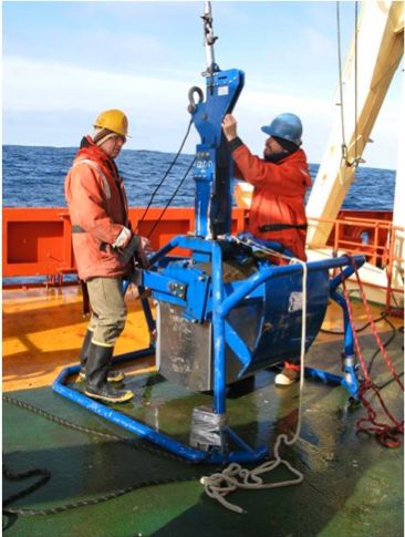
TABLE OF CONTENTS

Acknowledgments................................................................................... iii
Abstract................................................................................................... iv
List of Tables.......................................................................................... vii
List of Figures......................................................................................... viii
List of Abbreviations.............................................................................. ix
Chapter 1: Introduction........................................................................... 1
         An Introduction to Benthic Organisms…………………………………….. 1
         Benthic Pelagic Coupling on the Antarctic Shelf………………………….. 2
         A Benthic “Food bank” of Labile Organic Matter………………………….3
         Climate Change and the Western Antarctic Peninsula…………………….. 3
         Quantitative Reports on the Macrobenthos…………………………………6
         Objectives of this research…………………………………………………. 7
Chapter 2: Methods................................................................................. 9
         Field Methods……………............................................................................ 9
         Extraction…………………………………………………………………... 10
         Sieving the box-corer samples....................................................................... 11
         Sorting…........................................................................................................ 11
         Abundance…………………………………………………………………. 12
         Biomass………………………………………………………….................. 13
         Mean Macrofaunal Body Size……………………………………………... 14
         Graphing Programs………………………………………………………… 14
         Statistical Analyses of FOODBANCS 2 Data……………………………... 15
         Statistical Analyses of Mühlenhardt-Siegel (1988)………………………... 16
         Additional Data from Mühlenhardt-Siegel (1988)………………………… 16
         Analysis of Sea-Ice Data…………………………………………………… 17
         Sources of Error……………………………………………………………. 17

                                                               v
Chapter 4: Results & Discussion……………………………………… 19
         Abundance (N/m2) Results ………………………………………………... 19
         Discussion of Abundance …………………………………......................... 26
         Biomass (g/m2) Results…..……………………………………………........ 28
         Discussion of Biomass……………………………………………………... 34
         Mean Body Size (g/N) Results…………………………………….............. 38
         Discussion of Mean Body Size…………………………………………….. 41
         Conclusion…………………………………………………………………. 42
Appendix................................................................................................. 44
References............................................................................................... 51

                                                       vi
LIST OF TABLES
Table 1: CRS# Reference Information…………………………………………….. 10
Table 2: Taxonomic classifications from Mühlenhardt-Siegel (1988)…………….. 12
Table 3: Macrofaunal Abundance (N/m2)………………………………….……… 19
Table 4: Mean Taxon Abundance (N/m2)………………………………………….. 20
Table 5: Kruskal-Wallis Test of Macrofaunal (N/m2) along the WAPcs………….. 25
Table 6: Kruskal-Wallis Test of nsWAPcs (N/m2) vs. ssWAPcs (N/m2)………….. 25
Table 7: Macrofaunal Biomass (g/m2)…………………………………………….. 28
Table 8: Mean Taxon Biomass (g/m2)……………………………………………... 29
Table 9: Kruskal-Wallis Test of Macrofaunal (g/m2) along the WAPcs………….. 34
Table 10: Kruskal-Wallis Test of nsWAPcs (g/m2) vs. ssWAPcs (g/m2)………… 34
Table 11: Mean Body Size (g/N)…………………………………………………... 38
Table 12: Mean Taxon Body Size (g/N)…………………………………………… 39
Table 13: Kruskal-Wallis Test of Macrofaunal (g/N) along the WAPcs…………...40
Table 14: Kruskal-Wallis Test of nsWAPcs (g/N) vs. ssWAPcs (g/N)……………. 41
Table 15: Correlations of Latitude vs. Macrobenthic Parameters…………………. 44
Table 16: Correlations of Sea-Ice cover vs. Mean Macrobenthic Parameters……... 46
Table 17: Tests of Regional Differences from Mühlenhardt-Siegel (1988)……….. 49

                                         vii
LIST OF FIGURES
Figure 1: Chl a concentration from 1976 – 1986 vs. 1997 – 2006 on the WAPcs… 5
Figure 2: A Sorter’s view of sediment……………………………………………... 11
Figure 3: Total Macrofaunal Biomass (g/m2) from Mühlenhardt-Siegel (1988)….. 16
Figure 4: Stations of the Antarctic Peninsula from Mühlenhardt-Siegel (1988)…... 16
Figure 5: Total Macrofaunal Abundance by Sample…………………….…............ 20
Figure 6: Mean Abundance of Total Macrofauna………………………….……….21
Figure 7: Mean Polychaeta Abundance…………………………………….……… 21
Figure 8: Mean Mollusca Abundance………………………………………............ 22
Figure 9: Mean Crustacea Abundance………………………………………........... 22
Figure 10: Mean Echinodermata Abundance……………………………………… 23
Figure 11: Relative Abundance of Macrofauna at AA Stations…………………… 23
Figure 12: Relative Abundance of Macrofauna at B, F, & G Stations…………….. 24
Figure 13: Relative Regional Abundance from Mühlenhardt-Siegel (1988)….........24
Figure 14: Total Macrofaunal Biomass by Sample………………………….…….. 29
Figure 15: Mean Biomass of Total Macrofauna…………………………….……... 30
Figure 16: Mean Polychaeta Biomass………………………………………………30
Figure 17: Mean Mollusca Biomass……………………………………………….. 31
Figure 18: Mean Crustacea Biomass………………………………………………. 31
Figure 19: Mean Echinodermata Biomass…………………………………………. 32
Figure 20: Relative Biomass at AA Stations………………………………………. 32
Figure 21: Relative Biomass at B, F, and G Stations……………………….............33
Figure 22: Relative Regional Biomass from Mühlenhardt-Siegel (1988)…............. 33
Figure 23: Average Macrofaunal Body Size………………………....……………. 39
Figure 24: Average Echinodermata Body Size…………………….. ……………... 40
Figure 25: Mean Annual Sea-Ice Cover at stations AA, B, E, F, and G…………... 45
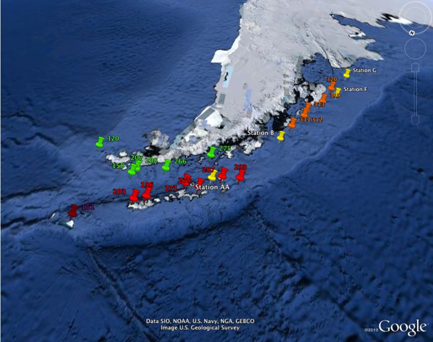
Figure 26: Station locations of FOODBANCS-2 and Mühlenhardt-Siegel (1988)... 47
Figure 27: Latitude, Depth, vs. Biomass from Mühlenhardt-Siegel (1988)……….. 48
Figure 28: The R/V Nathaniel B. Palmer and R/V Laurence M. Gould…… ……... 50
Figure 29: The Box-Corer Device…………………………………………………. 50
viii
LIST OF ABBREVIATIONS

AASW                Antarctic Surface Water
AFDW                Ash-free dry weight
cm                  Centimeters
Chl a               Chlorophyll concentration, measured in (mg/m3)
FOODBANCS           Food for the Benthos on the Antarctic Continental Shelf research
m                   meters
mg                  milligrams
NSF                 The National Science Foundation
nsWAPcs             Northern subregion of the WAP continental shelf (61° to 64.5°, S)
PAL-LTER            The Palmer Long Term Ecological Research Project
Preservation Sol.   4% Formaldehyde buffered with Sodium Tetraborate Decahydrate
POM                 Particulate Organic Matter
ssWAPcs             Southern subregion of the WAP (63.8° to 67.8°, S)
WAPcs               Western Antarctic Peninsula continental shelf

                                         ix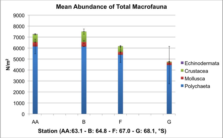
CHAPTER 1: INTRODUCTION

An Introduction to Benthic Organisms

       The polar regions of Antarctica are home to native and endemic fauna, both

within the terrestrial and marine environments. Antarctic organisms are of interest to

scientific researchers for multiple reasons, including their environmental isolation and

evolution in harsh environmental conditions (Hempel, 1985), as well as their response to

a rapidly changing climate (Clarke et al., 2007). This study focuses on the ecological

composition of the numerous marine organisms that live in or on the seafloor,

collectively referred to as the benthos. These benthic organisms, which are operationally

subdivided by their size, inhabit seafloors of all the oceans, including our area of study:

the continental shelf of the Western Antarctic Peninsula (WAPcs, 60°S to 75°S).

       The megafauna (or megazoobenthos) are a collection of benthic organisms

defined by sizes larger than 3cm or “large enough to be identified in bottom

photographs,” whereas macrofauna (the focus of this study) are defined as benthic

organisms greater in size than 500µm (0.5mm) yet smaller than the megafauna (Gage and

Tyler, 1992). Meiofauna, the smallest of the three size classes, are defined as organisms

within the size range of 62µm – 500µm (Giere, 2009). Some taxonomic groups, such as

copepoda and oligochaeta, are conventionally included in meiofauna, as are some groups

excluded from it (Hulings and Gray, 1971). Broad taxonomic phyla of benthos have been

used in this study and other scientific reports for categorizing patterns of macrofaunal

community structure and biomass, including the mollusca and echinodermata, as well as

classes such as the polychaeta and crustacea (Muhlenhardt-Siegel, 1988) based on their

relative dominance within the macrofauna.
                                              1
Benthic-Pelagic Coupling on the Antarctic Shelf
Suspension and deposit feeding benthic organisms, as well as sediment microbes,
rely on the particulate organic matter or phytodetrital “rain” generated from overlying
primary production. The relationship between the processes of the water column and the
benthic, seen in the transfer of surface nutrients to the seafloor, is referred to as Benthic-
Pelagic Coupling (Longhurst, 1983). The continental shelf of the WAP (WAPcs) is
especially impacted by these seasonal fluxes of particulate organic matter (POM) to the
seafloor. Reports from the Palmer Long-Term Ecological Research (PAL-LTER) study
area indicate very strong seasonality. The highest and lowest POM fluxes ever measured
among the world’s oceans were recorded on the Antarctic shelf in the austral summer and
austral wintertime, respectively (Karl, 1996). This seasonal flux, a consequence of
variations in sunlight between the austral summer and winter seasons (Eicken, 1992) has
ramifications for benthic ecosystem and structure (Clarke, 1985; Dayton, 1990; Arntz et
al., 1994; Smith et al., 2006) which may include changes in benthic biomass, feeding
behaviors, animal growth, developmental modes, reproductive strategies, bioturbation
rates and carbon burial (Smith et al. 2006, 2008).
In addition to increased photoperiod (i.e. duration of light) associated with pulsing
of organic matter from the euphotic zone of the Antarctic surface water (AASW), the
amount of primary productivity of the WAP shelf is also a function of sea-ice extent and
duration, as well as water stratification (Eicken, 1992; Smith et al., 2006). As a result,
benthic community structure will be an ecological end member to test our understanding
of Benthic-Pelagic coupling along the WAP shelf. Moreover, it’s expected that changes
in monthly and annual extent/duration of sea-ice, water stratification, and annual changes
2in primary productivity, as a function of latitude, will be reflected in measurements of
benthic community structure and composition, including biomass and abundance per
square meter.
A Benthic “Food bank” of Labile Organic Matter
Intense seasonal variation in primary productivity over the WAP continental shelf
(WAPcs) and the consequent strong pulses of POM, coupled with the low-temperatures,
are thought to be responsible for high standing concentrations of organic matter (Arntz et
al., 1994) on the WAPcs. However, multiple studies have found that macrofauna of the
WAP continental shelf consistently feed, grow, and reproduce throughout the year with
little variability despite seasonal variation in POM flux (Glover et al., 2008; Smith et al.,
2006, 2008; Galley et al., 2008; Sumida et al., 2008). Mincks et al. (2005) have
postulated that the underlying reason is due to the presence of a persistent “food bank” of
labile organic matter in sediments which accumulate at the seafloor and persist
throughout the year. As a consequence, Smith et al. (2006) argue that benthic parameters
such as inventories of labile organic matter and benthic biomass may act as “low-pass”
filters, only responding to longer-term changes in water column production, which will
allow researchers to examine how climate-driven changes act on a ecosystem not readily
perturbed.
Climate Change and the Western Antarctic Peninsula
Especially important to our understanding of Antarctic benthic ecology is to
figure out how rapid changes in the polar climate alter the regional benthic ecosystem.
3Major changes in the high-latitude region include, as a result of rapid regional warming
of the Antarctic Peninsula, the collapse of seven ice shelves in the past 50 years
(Vaughan and Doake, 1996), an increase in melt-water associated with rapid retreat of ice
shelves and marine glaciers (Clarke et al., 2007; Scambos et al., 2003) as well as a
decrease in sea-ice concentration and duration over the last two decades in the WAPcs
and Bellingshausen sea (Jacobs and Comiso, 1997; Smith and Stammerjohn, 2001;
Parkinson, 2002; Liu et al., 2004). Indeed, the rate of atmospheric temperature increase
on the WAP exceeds any other region of the Southern Hemisphere and is only paralleled
by northwestern North America and the Siberian Plateau in the Northern Hemipshere, --
of the three regions, only the WAP is maritime (Trenberth et al., 2007). Such rapid
changes in the atmosphere and AASW above the continental shelf of the WAP are
expected to induce changes in benthic processes, such as faunal abundance, biomass,
reproduction and recruitment, which are hypothesized to act as “low-pass” filters (Smith
and DeMaster, 2008).
Recently, Montes-Hugo et al. (2009) looked at biological changes associated with
regional climate change of the WAPcs, specifically changes in chlorophyll a (Chl a)
concentration associated with phytoplankton communities, as a function of water-column
mixing, which is in turn a function of ice-cover, cloudiness, and windiness. As seen in
Figure 1, Montes-Hugo et al. (2009) found that with respect to 1978 – 1986, satellite-
derived Chl a concentration has decreased by a factor of 2 in the northern subregion of
the WAPcs (nsWAPcs, 61° to 64.5° S, 59° to 65.8° W) and increased by a factor of 1.5 in
the southern subregion of the WAPcs (ssWAPcs, 63.8° to 67.8° S, 64.4° to 73.0° W).
4Figure 1: Changes in Chl a derived from satellite observation (dChls, mg m-3) between
1978 – 1986 and 1997 – 2006 along the WAPcs, from Montes-Hugo et al. (2009).
Montes-Hugo (2009) attributed the decrease in the nsWAPcs primary productivity
to increased cloudiness (decreased sunlight), persistently stronger winds, and decreased
summer sea-ice extent; conditions driving phytoplankton cells into a deeper mixed layer
with overall less light availability for photosynthesis. In comparison to the nsWAP, mean
annual sea-ice cover is greater in the ssWAP (Figure 25) and Montes-Hugo argues that in
this region any decrease in sea-ice cover over the surface mixed layer facilitates favorable
conditions for phytoplankton growth.
As a result of the rapid climate change occurring on the order of decades at the
WAPcs, an objective of our research is to better understand how the anthropogenic
warming may affect benthic pelagic coupling and consequently the macrobenthic
ecosystem. Through the comparison of our quantitative data of macrofauna to some of
the earliest quantitative data available on the benthic ecosystem of the WAPcs, we hope
5to better understand how the benthos have adapted to decadal regional warming of the
WAPcs and further predict how they will respond to a continuously changing climate.
Quantitative Reports on the Macrobenthos
The benthic ecosystem of the Antarctic continental shelf is characterized by
especially high biomass levels (Knox, 1994) and high variability (Gutt, 1991). To add to
this variability, much of the earlier published research on Antarctic benthos as a whole
lack quantitative data (Arnaud, 1992) due to qualitative sampling methods of the
macrobenthos (i.e., using Beam or Aggassiz trawls, Epibenthic sleds, Anchor Dredges,
etc). Furthermore, macrobenthic samples of the WAPcs have been retrieved
predominantly from shallow depths (comparison to the polychaeta dominated WAPcs. Inherently, early comparable studies for
quantitative analysis of macrofaunal communities for insight into climate change are
limited, especially since the Bellinghausen Sea west of the Antarctic Peninsula is one of
the least explored (Saiz et al., 2008).
In contrast to other benthic research of her time, Mühlenhardt-Siegel (1988)
provided an early example of quantitative macrobenthic research along a latidudinal
transect of the WAP from 60°S - 68°S from November, 1984 to April, 1985, which this
study was modeled after to provide a direct decadal comparison (Figure 26).
Mühlenhardt-Siegel (1988) collected eighty-six quantitative grab samples from 42
stations within a depth range of 60 – 850m, sieved macrofaunal samples on a 0.5mm
sieve, and taxonomically sorted them to the crustacea, mollusca, echinodermata, and
polychaeta, measuring both abundance and wet-weight per taxonomic group. Statistical
analyses were run on her raw data from the Antarctic Peninsula, and significant
interactions between latitude, depth, and biomass are shown (Figure 27) and discussed in
the Results and Discussion chapter.
Objectives of this research
The objective of this study is to quantify the macrofauna retrieved from box-corer
samples which were collected in March 2008 from the first cruise of the FOODBANCS-2
(Food for the Benthos on the Antarctic Continental Shelf) research program, in order to
compare our macrofaunal abundance and biomass data to both overlying sea-ice and
primary productivity data as well as to similar data obtained along the same latitudinal
gradient by earlier investigators in 1984 - 1985.
7Specifically, this study is designed to answer three questions:
1) How do total or taxon biomass, abundance, and mean body size of macrofauna of the
WAPcs vary as a function of latitude?
2) Is there any evidence of decadal variation in macrobenthic biomass and abundance
along the WAPcs?
3) How do biomass and abundance of macrofauna vary as a function of primary
productivity and mean annual sea-ice cover?
8CHAPTER 2: METHODS
Field Methods
The samples were collected as part of the second study of the Food for the
Benthos on the Antarctic Continental Shelf (FOODBANCS - 2) research program aboard
the R/V Laurence Gould (Figure 28, Appendix) from five stations, AA, B, E, F, and G
from 63.1°S to 68.1°S during March of 2008. All macrofaunal samples were obtained by
a 0.250 m2 box corer (Figure 29, Appendix), with a sub-core area of 0.25m x 0.25m or
0.0625 m2. Samples were preserved in 4% formaldehyde (or 10% formalin) buffered with
sodium tetraborate decahyrate. During the first cruise of FOODBANCS-2 in March 2008,
a total of 11 samples (three from station AA, two from station B, three from station F,
and three from station G) were used in this study. See Table 1 for each station, latitude
and longitude, as well as depth, CRS reference number, depth partition associated with
each sample, and sampling date.
Extraction
Samples were prepared for taxonomic sorting by the addition of Rose Bengal to
the preservation solution in the sample container. The red stain of Rose Bengal adhered
to the membrane of faunal species and allowed for easy identification and extraction of
the macrofauna from the sediment. After a period of at least 2.5 hours (overnight in most
cases) the stained samples were ready and prepared for extraction.
9Table 1: Station, Latitude and Longitude, Depth (in meters), CRS Reference number, Depth Partition (in centimeters), and Sampling Date
of each sample taken along the Western Antarctic Peninsula continental shelf (WAPcs).
10Sieving the box-corer samples
Macrofaunal samples were separated from the sediment via 500µm and 300µm
sieves, and the >500µm fraction and 500µm - 300µm fraction were separated and stored.
The fraction smaller than 300µm was not the focus of this research project, since it
contained by definition the meiofauna, and was subsequently stored. The >500µm
fractions containing the stained macrofauna were then prepared for sorting with
stereoscopic microscopes, and stored in preservation solution.
Sorting
The specific >500µm fraction was transferred to a petri dish filled with water
(Figure 2). Because the fumes of the preservation solution are suspected to be
carcinogenic, the sorter at the stereoscopic microscope transferred the sieved partition to
water and sorted the sediment in water.
Sorting of an individual sample at a particular depth required 4 - 24 hours of total
sorting time depending on the
concentration of macrofaunal
individuals and sediment
composition. All handling of
macrofaunal organisms was done
via fine forceps.
When a sample could not
be completely sorted in one
Figure 2: Sediment collection from a partition of a sample
with macrofaunal organisms already partially extracted.
11session, the sorted section of the sample was transferred to a permanent container filled
with the preservation solution. The remaining unsorted sample would be transferred to a
separate container in the same preservation solution until it could be sorted and
transferred to the same permanent container as the previously sorted material. Any
organisms found belonging to the meiofauna (e.g. copepoda, oligochaeta) were not
separated further but placed together into a “miscellaneous” vial. All other macrofaunal
taxa (e.g. tanaidacea, scaphopoda) were placed in their own taxon specific vial labeled
accordingly with the CRS reference number. All macrofaunal organisms were sorted
from the sediment according to major taxonomic classes similar to the classifications
used by Mühlenhardt-Siegel (1988) when applicable (Table 2).
Abundance
Abundance counts of polychaeta and other macrofauna were taken by counting
the macrofaunal head. If the head
Table 2: Macrofaunal taxonomic classifications from
Mühlenhardt-Siegel (1988). Crustacea (1 – 5), Mollusca (6 –
was not included in a fragment of a
8), Echinodermata (9 – 13), and Annelida (14).
macrofaunal individual, that
fragment was not counted in the
abundance, but rather was labeled
as a “fragment” of the particular
taxon order (e.g. “polychaete frag) to still be included in the wet weight biomass
measurements. Abundance counts were normalized by dividing the individuals per taxon
per sediment partition, by the number of sub-cores per partition and the area of the sub-
core (0.0625m2) to yield N/m2.
12Normalized abundance data were then statistically tested as a function of latitude.
Pearson’s, as well as Spearman’s rank (corrected for a non-parametric measure between
two variables) correlation coefficients were included in the analysis for both total
abundance (N/m2) as a function of latitude (Row 1, Table 15), as well as taxon abundance
per square meter as a function of latitude (Rows 4 – 7, Table 15). A Kruskal-Wallis test
(i.e. a non-parametric one-way ANOVA) was included to test for significant variation
between latitudes (Table 5), and the nsWAPcs and ssWAPcs (Table 6).
Biomass
Wet-weight biomass measurements were carried out after all taxa abundance
counts had been verified. Individual macrofaunal taxa were prepared for weighing by
emptying the vial of a taxon (e.g. polychaete) into a small petri dish. Two kimwipes were
placed adjacent to the stereomicroscope and used to absorb water from the macrofaunal
organisms and assure that no extra surface water was remaining on the exterior surface of
them (e.g. between the chelipads of a tanaid, or the chaete of a polychaete). Adjacent to
the kimwipes was a Denver Instrument APX-60 balance (accuracy +/- 0.2 mg, precision
0.1mg) with plasticized weighing paper on the stage (to assure little water absorption).
After macrofaunal individuals were dabbed on the kimwipes (which are very
efficient at absorption), placed on plasticized weighing paper and weighed, the
macrofauna and weighing paper were immediately placed in a water-filled petri dish to
prevent further drying.
Similar to the normalization of abundance, wet-weight biomass measurements
were also normalized to g/m2.
13Normalized biomass data were also tested as a function of latitude. Pearson’s, as
well as Spearman’s rank correlation coefficients were included in the analysis for both
total biomass (g/m2) as a function of latitude (Row 2, Table 15), as well as taxon biomass
(g/m2) as a function of latitude (Rows 8 – 11, Table 15). Kruskal-Wallis tests were also
included to test if biomass (g/m2) varied significantly between latitudes (Table 9) and
between the nsWAPcs and the ssWAPcs (Table 10).
Mean Macrofaunal Body Size
Because both individuals per square meter as well as grams per square meter
could be measured per taxon per sample, the mean individual body size was calculated
simply by taking the wet-weight biomass and dividing by abundance, i.e. g/m2 / N/m2 =
g/N, or mass per individual.
Total and taxa g/N from each sample were correlated with latitude (Row 3, Table
15; Rows 12 - 15, Table 15). In addition, mean body size was tested for statistical
variation along the WAPcs (Table 13) and between the nsWAPcs and ssWAPcs (Table
14). In addition, a visual representation of the average taxon body size with latitude was
produced (Figures 23 & 24).
Graphing Programs
Abundance (N/m2), biomass (g/m2), and mean body size (g/N) were calculated in
Microsoft Excel 2008. Graphing programs used included Microsoft Excel 2008 and
Matlab R2008b. The standard error associated with each station was calculated from the
standard deviation divided by the sample size for each station (i.e. 3, for station AA).
14Matlab R2008b was used to produce the 3D scatter plot (Figure 27) of data from
Mühlenhardt-Siegel (1988).
Statistical Analyses of FOODBANCS 2 Data
Data from FOODBANCS 2 were tested for statistical significance in Minitab
v.16. Primary tests for statistical significance included non-parametric correlations
(Spearman’s ranked correlation coefficient) between latitude and: total N/m2 per sample
per station, total g/m2 per sample per station, and total g/N per sample per station (Rows
1 – 3 in Table 15; original data in Tables 3, 7, and 11, respectively). Other tests included
non-parametric correlations between latitude and: taxon abundance per square meter
(Rows 4 – 7, Table 15), taxon biomass per square meter (Rows 8 – 11, Table 15), and
taxon mean body size per square meter (Rows 12 – 15, Table 15). In addition to the
Spearman’s ranked correlation coefficient, the parametric Pearson’s correlation
coefficient was included for comparison. Both correlation coefficients include P-values
corresponding to significance (Statistical Analyses of Mühlenhardt-Siegel (1988)
Data from Mühlenhardt-Siegel (1988) were also tested for significance in Minitab
v.16. Latitude, depth, and biomass data (Figure 3) from Mühlenhardt-Siegel (1988) at
individual stations along
the Antarctic Peninsula
(Figure 4) were tested for
significant regressions. For
a comparison of the
locations of stations used in
FOODBANCS-2 and
Figure 3: Total macrofaunal biomass (g/m2) per sample per region
from Mühlenhardt-Siegel (1988). X – axis values indicate sampling Mühlenhardt-Siegel (1988),
depth, y-axis indicates biomass (g/m2). “D” region corresponds to the
“northern Antarctic peninsula,” “C” to “South Sheltand Islands,” see Figure 26.
and “E,” to the “southern Antarctic peninsula.”
Additional Data from Mühlenhardt-Siegel (1988)
Additional data used from Mühlenhardt-Siegel (1988) include relative and mean
abundance (N/m2) (Figure 13) as
well as relative and mean biomass
(g/m2) (Figure 22), for the northern
and southern subregions of the
WAPcs (nsWAPcs and ssWAPcs,
respectively. A table of Mann-
Whitney-U-tests testing for
Figure 4: Stations where latitude, depth, and biomass
were recorded from Mühlenhardt-Siegel (1988) along
the Antarctic Peninsula.
16statistical significance in biomass (g/m2) and abundance (N/m2) between regions of the
Antarctic Peninsula was also included (Table 17).
Analysis of Sea-Ice Data
Lastly, additional sea-ice data were included (Figure 25) to determine if mean
total and taxon abundances (N/m2), biomass (g/m2), and mean body size (g/N)
statistically correlate (Spearmean’s Rank) with annual sea-ice cover (in mo/yr) by using
mean values of sea-ice cover (months/year, 4-data points) at each AA, B, F, and G
station. The results may be found in the Appendix (Table 16).
Sources of Error
Most sources of error or variability in this project originate from the nature of the
study. Variability in sampling depths between stations from Mühlenhardt-Siegel (1988)
and the resulting variability in biomass measurements from those stations introduce a
source of error for comparison purposes of the macrobenthos between 1985 and 2008.
While a statistical test for decreasing biomass with latitude and depth was significant (P =
0.05) there was still documented variability between similar latitudes and depth (Figure
27). In addition, “wet-weight” biomass measurements are criticized as more prone to
error compared to ash-free dry-weight (AFDW), however for comparison purposes to
Mühlenhardt-Siegel (1988), as well as for preservation of specimens, wet-weight
measurements were used.
Other sources of potential error in constructing decadal changes in this project
include the limited sampling and general lack of quantitative knowledge on the
17macrofauna of the WAPcs and Bellinghausen Sea prior to this study (Arnaud et al., 1992;
Pipenberg et al., 2002). Additional macrofaunal sampling beyond the 11 samples used in
FOODBANCS 2 (Table 1) would strengthen statistical testing, however considering that
over 10,000 macrofaunal organisms were extracted from these 11 samples, a limitation to
this study is the considerable amount of time required for macrofaunal extraction from
the sediment alone.
Other sources of error include the extraction of the macrofauna from the
sediment. It’s very likely that some individual macrofaunal organisms were overlooked
and not extracted from the sediment. However, because every sample was rigorously
examined for individual organisms, any remaining macrofauna will likely not alter any
general trends. However, further examination is likely to refine the standard error
associated with each taxon per station.
For records purposes, this study extracted numerous organisms associated with
taxonomic and size-based definitions that exclude the macrofauna. Any organisms
taxonomically belonging to meiofauna (Hulings and Gray, 1971) were not included in
this study (e.g. copepoda, nematoda, foramnifera, oligochaeta etc.), and a single
megabenthic organism, Limopsis marionensis, found in the CRS 968 0 – 5cm partition
(Station B, Table 1) was not included due to it size (> 4cm) and incomparable status to
the macrozoobenthos of Mühlenhardt-Siegel (1988). For reference purposes, the
individual L. marionensis organism weighed 22.7755 grams (Figure 17).
18CHAPTER 4: RESULTS & DISCUSSION
Overall, 10,260 macrofaunal organisms were extracted from a total of 11 samples
belonging to four different stations (AA, B, F, and G) spanning 63.1°S to 68.1°S along
the WAPcs. After briefly presenting the results of each respective macrobenthic
parameter, decadal and latitudinal variation of macrofaunal abundance (N/m2), biomass
(g/m2), and mean body size (g/N) along the WAPcs will be discussed in detail,
respectively, in relation to overlying primary productivity and mean annual sea-ice cover.
Abundance (N/m2) Results
Normalized abundance (N/m2) for each particular taxa (Table 2) were compiled to
broad taxonomic group (Table 3) and graphed (Figure 5). The mean total abundance
(N/m2) per station was also determined (Table 4) and graphed (Figure 4) as well as
individual mean abundances per taxon for each station (Figures 6 – 9).
Table 3: Normalized abundance (N/m2) for polychaeta, mollusca, crustacea, and echinodermata per
station. Total abundance per square meter was calculated for each sample (CRS#) for each station
(last column).
19Figure 5: Total macrofaunal abundance counts (N/m2) for polychaeta, mollusca, crustacea, and
echinodermata per sample. Total (N/m2) per sample is reflected in the height of the column.
Table 4: Abundance (N/m2) at each individual of polychaeta, mollusca, crustacea, echinodermata,
along with the standard error (S.E) associated with each taxa. The mean values of abundance (N/m2)
ranged from 4768 – 7504 N/m2.
20Figure 6: Mean abundance of total polychaeta, mollusca, crustacea, and echinodermata per square
meter (N/m2) at each individual station. Mean values ranged from 4768 – 7504/m2. Error bars reflect
the standard error for each taxa at each station.
Figure 7: Mean polychaeta abundance per square meter (N/m2) for stations AA, B, F,
and G. Error bars reflect the standard error at each station.
21Figure 8: Mean mollusca abundance per square meter (N/m2) for stations AA, B, F,
and G. Error bars reflect the standard error at each station.
Figure 9: Mean crustacea abundance per square meter (N/m2) for stations AA, B, F,
and G. Error bars reflect the standard error at each station.
22Figure 10: Mean echinodermata abundance per square meter (N/m2) for stations AA,
B, F, and G. Error bars reflect the standard error at each station.
In addition, relative abundance (N/m2) per subregion of the WAPcs was also
generated (Figure 11 & 12) for comparison against relative abundance (N/m2) per
subregion compiled by Mühlenhardt-Siegel (1988) (Figure 13).
Figure 11: Relative abundances of macrofauna (N/m2) for AA Stations, reflecting the
nsWAPcs. Polychaeta: 84%, Crustacea: 10%, Mollusca: 5%, Echinodermata: 1%. Total
mean N/m2: 7280.
23Figure 12: Relative abundances of macrofauna (N/m2) for B, F, and G Stations, reflecting the ssWAPcs. Polychaeta: 87%, Crustacea: 8%, Mollusca: 5%, Echinodermata:
Finally, latitudinal variation of total macrofaunal abundance (N/m2) both along

the WAPcs (Table 5) and between the nsWAPcs and the ssWAPcs (Table 6) were tested

for statistical significance via Kruskal-Wallis tests, as described in the Methods:

Statistical Analyses of FOODBANCS 2 Data. Results indicate no significant variation

along the WAPcs, nor between the nsWAPcs and the ssWAPcs (P > 0.05).

Table 5: Kruskal-Wallis Test on total macrofaunal N/m2 vs. latitude (63.1°S – station AA, 64.8°S –
station B, 67.0°S – station F, and 68.1°S – station G). P-value of 0.488 indicates that macrofaunal
abundance per square meter does significantly vary between latitudinal stations.

Table 6: Kruskal-Wallis Test on variation of total macrofaunal N/m2 between the nsWAPcs
(represented by macrofaunal N/m2 of station AA) and the ssWAPcs (macrofaunal N/m2 of
stations B, F, and G with average latitude of 66.6°S). P-value of 0.280 indicates that there is no
significant variation in total macrofaunal N/m2 between the nsWAPcs and the ssWAPcs

                                                   25
Discussion of Abundance
In response to our first question, “Does total or taxon abundance vary as a
function of latitude?” our results from the Kruskal-Wallis test (Table 5) indicate no
significant variation in total abundance (N/m2) with latitude, nor between the nsWAP and
the ssWAP (Table 6), indicated by the P-values of 0.487 and 0.280, respectively. In
addition, using Spearman’s ranked correlation coefficient we found a rs of -0.445 and a P-
value of 0.170 (Row 1, Table 15) which was not statistically significant (P < 0.05).
It should be noted, however, that when analyzing taxon abundances (N/m2) our
study found significant negative correlations in decreasing trends of mollusca abundance
(N/m2) (Figure 8; P-value of 0.025 and rs of -0.666, Row 5, Table 15) and in crustacea
abundance (N/m2) (Figure 9; P-value of 0.002 and rs of -0.831, Row 6, Table 15) with
increasing latitude. We did not find any significant correlations with polychaeta or
echinodermata abundance (N/m2) (Figure 7 & Figure 10; Rows 4 & 7, Table 15). Overall,
our results indicate little variation of macrofaunal abundance (N/m2) with latitude or
between the nsWAPcs or the ssWAPcs.
In response to our second question “Is there any evidence of decadal variation in
macrobenthic abundance along the WAPcs?” In 1984 – ’85, Mühlenhardt-Siegel (1988)
found an average of 8642 N/m2 in the nsWAPcs, an average of 2050 N/m2 in the
ssWAPcs, and a significant variation in macrofaunal abundance between these regions of
the WAPcs (Figure 13; D vs. E, Abundance, Table 17). In comparison, our study found
an average of 7280 N/m2 in the nsWAPcs (Figure 11) vs. an average of 5980 N/m2 in the
ssWAPcs (Figure 12) and no significant variations in total abundance with or between
latitudes (Tables 5 - 6; Row 1, Table 15).
26Intriguingly, the abundance (N/m2) found in our study at the ssWAPcs (stations B,
F, and G) is over twice that found in the ssWAP in 1985 (Figure 12 vs. Figure 13). In
addition, we found much greater relative abundances of polychaeta, and less so of
mollusca, crustacea, and echinodermata at both nsWAP and ssWAP sampling sites
(Figures 11 & 12) compared to Mühlenhardt-Siegel (1988) (Figure 13), suggesting a
change in macrobenthic diversity in the ssWAPcs since 1985. Overall, Mühlenhardt-
Siegel (1988) found a statistically significant greater abundance of macrofauna in the
nsWAPcs compared to the ssWAPcs (“D vs. E,” Abundance, Table 17) and a more
taxonomically diverse assemblage of macrofauna in both regions. Samples from
FOODBANCS-2 have comparatively less taxonomic diversity and abundance (N/m2) in
the nsWAPcs, and less taxonomic diversity and greater abundance (N/m2) in the
ssWAPcs, suggesting a decadal homogenization of the WAPcs since 1985.
In response to last question, “Do total and taxon abundance vary as a function of
primary productivity and sea-ice cover,” our results show an increase of abundance N/m2
in the ssWAPcs and a decrease in the nsWAPcs since 1985, which is consistent with
changes in decadal primary productivity rates on the WAPcs (Figure 1) from Montes-
Hugo (2009). These results suggest a link that with increased primary production over-
time there are increases in macrofaunal abundance (N/m2). However, also important to
note is that overall macrofaunal abundances (N/m2) are still higher in the nsWAPcs
compared to the ssWAPcs, suggesting that despite a strong decadal decrease in Chl a
production in the nsWAPcs and increase in the ssWAP, overall production levels are still
higher in the nsWAPcs compared to the ssWAPcs, most likely due to changes in mean
annual sea-ice cover in the ssWAP compared to the nsWAPcs (Montes-Hugo, 2009).
27Overall, this is evidence that macrofaunal abundance N/m2 is a function of the overall
amount as well as the rate of change in primary productivity of the WAPcs, which is
further driven by changes in mean annual sea-ice cover (Eicken et al., 1992; Smith et al.,
2006) in addition to other factors such as cloudiness and wind strength (Montes-Hugo et
al., 2009)
Biomass (g/m2) Results
Normalized biomass (g/m2) for each particular taxa (Table 2) were compiled to
broad taxonomic group (Table 7) and graphed (Figure 14). The mean total biomass
(g/m2) per station was also determined (Table 8) and graphed (Figure 15) as well as
individual mean abundances per taxon for each station (Figures 16 – 19).
Table 7: Normalized biomass (g/m2) for polychaeta, mollusca, crustacea, and echinodermata per
station. Total biomass per square meter was calculated for each sample (CRS#) for each station
(last column).
28Figure 14: Total macrofaunal biomass (g/m2) for polychaeta, mollusca, crustacea, and echinodermata
per sample. Total (g/m2) per sample is reflected in the height of the column.
Table 8: Biomass (g/m2) at each individual of polychaeta, mollusca, crustacea, echinodermata, along
with the standard error (S.E) associated with each taxa. The mean values of biomass (g/m2) ranged
from 7.64 – 27.01 g/m2.
29Figure 15: Mean biomass of total polychaeta, mollusca, crustacea, and echinodermata per square meter
at each individual station. Total mean values ranged from 7.64 – 27.01 g/m2. Error bars reflect the
standard error for each taxa at each station.
Figure 16: Mean polychaeta biomass per square meter (g/m2) for stations, AA, B, F,
and G. Error bars reflect the standard error at each station.
30Figure 17: Mean mollusca biomass per square meter (g/m2) for stations, AA, B, F, and
G. Error bars reflect the standard error at each station.
Figure 18: Mean mollusca biomass per square meter (g/m2) for stations, AA, B, F, and
G. Error bars reflect the standard error at each station.
31Figure 19: Mean echinodermata biomass per square meter (g/m2) for Station, AA, B, F,
and G. Error bars reflect the standard error at each station.
In addition, relative biomass (g/m2) per subregion of the WAPcs was also
generated (Figure 20 & 21) for comparison against relative biomass (g/m2) per subregion
compiled by Mühlenhardt-Siegel (1988) (Figure 22).
Figure 20: Relative biomass of macrofauna (g/m2) for AA Stations, reflecting the
nsWAPcs. Polychaeta: 43%, Crustacea: 12%, Mollusca: 6%, Echinodermata: 39%. Total
mean g/m2: 27.01.
32Figure 21: Relative biomass of macrofauna (g/m2) for B, F, and G Stations, reflecting
the ssWAPcs. Polychaeta: 92%, Crustacea: 3%, Mollusca: 4%, Echinodermata: 1%.
Total mean g/m2: 10.19.
Figure 22: Relative macrofaunal biomass (g/m2) per region. Region “D,” the “northern Antarctic
Peninsula” with a mean g/m2 of 111.12 and Region “C,” the “South Shetland Islands” with a mean
g/m2 of 57.13 combined reflect the nsWAPcs. Region “E” reflects the ssWAPcs with a mean g/m2 of
9.06 g/m2. Legend provides thatching type associated with broad taxonomic group. From
Mühlenhardt-Siegel (1988).
33Finally, latitudinal variation of total macrofaunal biomass (g/m2) both along the
WAPcs (Table 9) and between the nsWAPcs and the ssWAPcs (Table 10) was tested for
statistical significance via Kruskal-Wallis tests, as described in the Methods: Statistical
Analyses of FOODBANCS 2 Data. Results indicate significant variation along the
WAPcs and between the nsWAPcs and the ssWAPcs (P < 0.05).
Table 9: Kruskal-Wallis Test on total macrofaunal g/m2 vs. latitude. P-value of 0.004 indicates that
macrofaunal biomass per square meter does significantly vary between latitudinal stations.
Table 10: Kruskal-Wallis Test on variation of total macrofaunal g/m2 between the nsWAPcs
(represented by macrofaunal g/m2 of station AA) and the ssWAPcs (macrofaunal g/m2 of stations
B, F, and G with average latitude of 66.6°S). P-value of 0.001 indicates significant variation in
total macrofaunal g/m2 between the nsWAPcs and the ssWAPcs
Discussion of Biomass
Our first question asks whether total or taxon biomass varies as a function of
latitude. The results from the Kruskal-Wallis test indicate that total biomass values (g/m2)
vary between latitudes (Table 9) at a significance value of P = 0.004. Spearman’s ranked
34correlation coefficient also show that the total macrofaunal biomass (g/m2) varies as a
function of latitude (rs of -0.642 and P-Value of 0.033, Row 2, Table 15). In addition, a
Kruskal-Wallis test of macrofaunal biomass (g/m2) indicates a very significant variation
(P-value of 0.001) between the nsWAPcs and the ssWAPcs (Table 10).
Analysis reveals that biomass (g/m2) of every taxon, including mollusca (Figure
17; rs of -0.820, P-value of 0.002, Row 9, Table 15), crustacea (Figure 18; rs of -0.829, P-
value of 0.002, Row 10, Table 15), and echinodermata (Figure 19; -0.609, P-value of
0.047, Row 11, Table 15) with the exception only of the polychaeta (Figure 16; rs of -
0.356, P-value of 0.282 Row 8, Table 15) significantly declines with increasing latitude.
These total and taxon biomass values are also negatively correlated with mean annual
sea-ice cover from (Figure 25) suggesting an association with a latitudinal decrease in
primary productivity.
Compared to the results of Mühlenhardt-Siegel (1988), both data sets reveal a
significant difference in biomass (g/m2) between the nsWAPcs and the ssWAPcs.
Mühlenhardt-Siegel (1988) found an average biomass of 57.13 g/m2 in the South
Shetland Islands and 111.12 g/m2 in the northern Antarctic Peninsula (Figure 22).
Mühlenhardt-Siegel (1988) also found an average biomass of 9.06 g/m2 in the ssWAPcs
(Figure 22). In comparison, we found a mean biomass of 27.01 g/m 2 in the nsWAPcs
(Figure 20) and of 10.19 g/m2 in the ssWAPcs (Figure 21). These regional differences
suggest the persistence of a latitudinal gradient in biomass over the past 26 years between
the northern and southern subregions of the WAPcs.
When further examining which taxonomic group dominates the biomass
measurements, we found many more polychaeta taxonomically dominating the biomass
35of the ssWAPcs (92%, Figure 21) compared to the biomass data of the ssWAPcs (~16%,
“E,” Figure 22) from Mühlenhardt-Siegel (1988). The biomass of the ssWAPcs from
Mühlenhardt-Siegel (1988) is dominated by echinodermata, whereas our data from the
ssWAPcs show the echinodermata contributing only 1% to biomass (Figure 21). Such a
drastic shift in the taxonomic composition of the biomass of the ssWAPcs could be the
result of either a low-probability sampling error (eight samples were taken both in the
FOODBANCS-2 and Mühlenhardt-Siegel (1988) study region of the ssWAPcs), or the
result of a major ecological shift in the macrobenthic community structure of the
ssWAPcs. It should be noted that in comparison, the taxonomic composition of the
nsWAP looks similar to that of 26 years ago (Figure 20, “D and C” Figure 22).
This brings us to one important difference in comparing average biomass data
from the FOODBANCS 2 project of 2008 with the average biomass from Mühlenhardt-
Siegel (1988). In 1984 -‘85 the average biomass of the nsWAP is over twice as large as
that of measured in 2008, whereas the average biomass of the ssWAP is lower (9.06 g/m2
compared to 10.19 g/m2) and taxonomically much different (Figure 21, “E” Figure 22).
Such a difference suggests the presence of a persisting latitudinal decline in
macrobenthic biomass with increasing latitude along the WAPcs, but a decrease in the
“steepness” of the cline since 1985. One explanation may be that the macrobenthic
biomass parameter is responding heavily to the overlying primary productivity, which has
decadally decreased in the nsWAPcs and increased in the ssWAPcs as a function of
decreased mean annual sea-ice cover (Montes-Hugo et al., 2009).
To test whether these sub-regional changes were present, i.e., that the slope of the
macrobenthic decrease in biomass with increasing latitude was lessening, we statistically
36tested the sampling of Mühlenhardt-Siegel (1988) for any significant regressions between
latitude, depth, and biomass (see Statistical Analyses of Mühlenhardt-Siegel (1988)).
After performing a multiple regression of biomass (response) with latitude and depth
(predictors) on all sampling stations (which are most heavily concentrated in the nsWAP,
Figure 4) from Mühlenhardt-Siegel (1988), we found a significant regression (P-value =
0.05) and the equation “Biomass = 2275.43 – 31.8192*(Latitude) – 0.381964*(Depth)”
(Figure 27). Using this equation we would predict a biomass of 46.86 g/m2 from 26 years
ago at the exact location (63.1° S) and depth of station AA (578m), which is almost twice
our value of 27.01 g/m2. The equation fails to accurately predict the biomass at the
ssWAP from 26 years ago, but given that the equation is based on sampling that occurs
primarily in the nsWAP (only four sampling stations from Mühlenhardt-Siegel (1988) are
located in the ssWAP) this is not surprising.
Overall, the shift in taxonomic composition and minor increase in biomass (g/m2)
of the ssWAP from 1985 to 2008 (Figure 21, “E” Figure 22) are accompanied by a large
suspected decrease in biomass (g/m2) in the nsWAP from 1985 to 2008 (46.86g/m2 to
27.01g/m2). Thus, while certainly not conclusive, there is evidence for a change in the
slope of the latitudinal gradient in biomass (g/m2) corresponding to a decadal increase in
primary productivity in the ssWAPcs and decrease in the nsWAPcs, and further
homogenization of the macrobenthic community along the WAPcs (Montes-Hugo et al.,
2009) similar to trends in abundance (N/m2).
Finally, our last question: “how does the macrobenthic biomass (g/m2) vary as a
function of mean annual sea-ice cover?” Our results show significant variation of total
macrofaunal biomass (g/m2) between stations (Kruskal Wallis test, Table 9) and between
37You can also read